Non-Markovian band-edge effect and entanglement generation of quantum dot excitons coupled to nanowire surface plasmons

Abstract

The radiative decay of quantum dot (QD) excitons into surface plasmons in a cylindrical nanowire is investigated theoretically. Maxwell’s equations with appropriate boundary conditions are solved numerically to obtain the dispersion relations of surface plasmons. The radiative decay rate of QD excitons is found to be greatly enhanced at certain values of the exciton bandgap. Analogous to the decay of a two-level atom in the photonic crystal, we first point out that such an enhanced phenomenon allows one to examine the non-Markovian dynamics of the QD exciton. Besides, due to the one dimensional propagating feature of nanowire surface plasmons, remote entangled states can be generated via super-radiance and may be useful in future quantum information processing.

The collective motions of an electron gas in a metal or semiconductor are known as plasma oscillations. In the presence of surfaces, not only the bulk modes are modified, but also surface modes can be created¹. When a light wave strikes a metal surface, a surface plasmon polariton—a surface electromagnetic wave that is coupled to plasma oscillations, can be excited. Investigations of the dispersion relations of surface plasmons for different geometries have been reported² since the 1970s. Recently, great attention has been focused on the so-called plasmonics since surface plasmons reveal strong analogies to light propagation in conventional dielectric components³. For examples, it is now possible to confine them to subwavelength dimensions⁴ and develop novel approaches for waveguiding below the diffraction limit⁵. The useful subwavelength confinement, single mode operation⁶, and relatively low power propagation loss⁷ of surface plasmon polaritons could be applied to miniaturize photonic circuits⁸. High surface plasmon field confinement was also used to demonstrate an all-optical modulator⁹.

Plasmon induced modification of the spontaneous emission (SE) rate is naturally an extended issue. Arnoldus et al. theoretically investigated the atomic fluorescence and spontaneous decay near a metal surface¹⁰. Strong enhancement of fluorescence due to surface plasmons was also observed¹¹. This enhanced fluorescence was considered as a possible method to improve the quantum efficiency of light-emitting devices. R. Paiella recently proposed tunable surface plasmons in silver-GaN multiple layers to increase the radiative recombination rate and equivalently the photoluminescence efficiency¹². Strong and coherent coupling between individual optical emitters and guided plasmon excitations in conducting nanowires at optical frequencies was also pointed out¹³ and may be used as a novel single-photon transistor¹⁴.

In this work, we investigate the SE rate of a II-VI colloidal QD (nanocrystals) exciton coupled to surface plasmons in a silver nanowire. Radiative decay of a QD exciton into different modes of surface plasmons is considered separately. The emission rate is found to be greatly enhanced at certain values of QD exciton bandgap, which is similar to the band-edge effect in photonic crystals. In addition, application of such a system in generating remote entangled states is also pointed and may be useful in future quantum information processing.

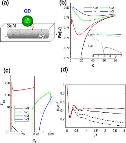
Figure 1: (a) Schematic view of the model: a silver nano-wire is embedded inside GaN material and a QD (quantum dot) is put on top of it. (b) Dispersion relations of surface plasmons for the first few modes. The units for vertical and horizontal lines are$\ \Omega=\omega/\omega_{p}$ and $K=k_{z}c/\omega_{p}$ . (c) Corresponding (Markovian) SE rates into surface plasmons. (d) Non-Markovian decay dynamics of QD excitons for $\delta=0.2\beta$ (black line), $0.4\beta$ (dotted line), and $0.8\beta$ (dashed line). As $\delta=0,$ the red line represents the result for the contribution from $n=1$ mode.

Dispersion relations of surface plasmons.–Consider now a colloidal CdSe/ZnS QD near a cylindrical silver nanowire with radius $a$. The QD and nanowire are assumed to be separated by a GaN layer¹⁵ as shown in Fig. 1 (a). One of the main reasons to choose a CdSe/ZnS QD exciton as the two-level emitter is that it is now possible to isolate single colloidal QD and measure its exciton lifetime¹⁶. The other reason is that its exciton bandgap is around $2eV$ to $2.5eV$, depending on the size and environment of the dot¹⁷. The plasmon energy $\hbar\omega_{p}$ of bulk silver is $3.76~{}eV$ with the corresponding saturation energy $\hbar\omega_{p}/\sqrt{2}\approx 2.66eV$ in the dispersion relation¹⁸. As we shall see below, variations of the dispersion relations in energy just match the exciton bandgap of colloidal CdSe/ZnS QDs.

Surface plasmon modes are created due to the nonzero local charge density on the surface of a nanowire. The n-th surface plasmon mode’s components of the electromagnetic field at the surface can be obtained by solving Maxwell’s equations in a cylindrical geometry ($\rho~{}$and $\varphi$ denote the radial and azimuthal coordinates, respectively) with the appropriate boundary conditions²:

$$E_{\rho}=[\frac{ik_{z}}{K_{\xi}}\frac{d\psi_{n}^{\xi}(K_{\xi}\rho)}{d(K_{\xi}\rho)}A_{n}^{\xi}-\frac{\mu_{\xi}\omega n}{K_{\xi}^{2}\rho}\psi_{n}^{\xi}(K_{\xi}\rho)B_{n}^{\xi}]\phi_{n},$$

$$E_{\varphi}=-[\frac{nk_{z}}{K_{\xi}^{2}\rho}\psi_{n}^{\xi}(K_{\xi}\rho)A_{n}^{\xi}-\frac{i\mu_{\xi}\omega}{K_{\xi}}\frac{d\psi_{n}^{\xi}(K_{\xi}\rho)}{d(K_{\xi}\rho)}B_{n}^{\xi}]\phi_{n},$$

$$E_{z}=[\psi_{n}^{\xi}(K_{\xi}\rho)A_{n}^{\xi}]\phi_{n},$$

$$H_{\rho}=[\frac{n(K_{\xi}^{2}+k_{z}^{2})}{\mu_{\xi}\omega K_{\xi}^{2}\rho}\psi_{n}^{\xi}(K_{j}\rho)A_{n}^{\xi}+\frac{ik_{z}}{K_{\xi}}\frac{d\psi_{n}^{\xi}(K_{\xi}\rho)}{d(K_{\xi}\rho)}B_{n}^{\xi}]\phi_{n},$$

$$H_{\varphi}=[\frac{i(K_{\xi}^{2}+k_{z}^{2})}{\mu_{\xi}\omega K_{\xi}}\frac{d\psi_{n}^{\xi}(K_{\xi}\rho)}{d(K_{\xi}\rho)}A_{n}^{\xi}-\frac{nk_{z}}{K_{\xi}^{2}\rho}\psi_{n}^{\xi}(K_{\xi}\rho)B_{n}^{\xi}]\phi_{n},$$

$$H_{z}=[\psi_{n}^{\xi}(K_{\xi}\rho)B_{n}^{\xi}]\phi_{n},$$ (1)

with

$$K_{\xi}^{2}=\omega^{2}\epsilon_{\xi}(\omega)/c^{2}-k_{z}^{2}\text{ \ (}\xi=I\text{ or }O\text{)},$$

$$\psi_{n}^{I}(K_{I}\rho)=J_{n}(K_{I}\rho),~{}\psi_{n}^{O}(K_{O}r)=H_{n}^{(1)}(K_{O}\rho),$$

$$\phi_{n}=exp(in\varphi+ik_{z}\emph{z}-i\omega t),$$

where $J_{n}(K_{I}\rho)$ are $H_{n}^{(1)}(K_{O}\rho)$ are Bessel and Hankel functions, respectively. I (O) stands for the component inside (outside) the wire. The dielectric function is assumed as ${\epsilon}(\omega)=\varepsilon_{\infty}[1-\frac{\omega_{p}^{2}}{\omega(\omega+i/\tau)}]$, where $\epsilon_{\infty}=9.6$ (for Ag), $\epsilon_{\infty}=5.3$ (for GaN), and $\tau$ is the relaxation time due to ohmic metal loss¹². The magnetic permeabilities $\mu_{I,O}$ are unity everywhere since we consider nonmagnetic materials here. $A_{n}^{\xi}$ and $B_{n}^{\xi}$ are constants to be determined by normalizing the electromagnetic field to the vacuum fluctuation energy, $\int\epsilon(\left|E_{\rho}\right|^{2}+\left|E_{\varphi}\right|^{2}+\left|E_{z}\right|^{2})d\mathbf{r}=\hbar\omega(\mathbf{k})$, and matching the boundary conditions. The dispersion relations of the surface plasmons are thus obtained by solving the following transcendental equation numerically:

$$S(k_{z},\omega)=$$

$$[\frac{\mu_{I}}{K_{I}a}\frac{J_{n}^{\prime}(K_{I}a)}{J_{n}(K_{I}a)}-\frac{\mu_{O}}{K_{O}a}\frac{H_{n}^{(1)\prime}(K_{O}a)}{H_{n}^{(1)}(K_{O}a)}][\frac{(\omega/c)^{2}\varepsilon_{I}(\omega)}{\mu_{I}K_{I}a}\frac{J_{n}^{\prime}(K_{I}a)}{J_{n}(K_{I}a)}$$

$$-\frac{(\omega/c)^{2}\varepsilon_{O}(\omega)}{\mu_{O}K_{O}a}\frac{H_{n}^{(1)\prime}(K_{O}a)}{H_{n}^{(1)}(K_{O}a)}]-n^{2}k_{z}^{2}[\frac{1}{(K_{O}a)^{2}}-\frac{1}{(K_{I}a)^{2}}]^{2}$$

$$=0.$$ (2)

The dispersion relations for various modes $n$ are shown in Fig. 1 (b) with effective radii $R=0.1$. One unit of the effective radii $R$ ($\equiv\omega_{p}a/c$) is roughly equal to $53.8~{}nm$. The behavior for the $n=0$ mode is very similar to the two-dimensional case¹⁸, i.e. $\Omega$ gradually saturates with increasing wave vector $k_{z}$. This is because the fields for the $n=0$ mode are independent of the azimuthal angle $\varphi$. However, the behavior for the $n\neq 0$ modes are quite different. The first interesting point are the discontinuities around $\omega/c\approx k_{z}$. Further analysis shows that the solutions of $\omega$ are “almost real”¹⁹ as $k_{z}>Re[\omega]/c$. Thus, the first Hankel function of order n, $H_{n}^{(1)}(K_{\xi}\rho)$, decays exponentially. This means the surface plasmons in this regime are confined on the surface (bound modes). For $k_{z}$ $<Re[\omega]/c$, however, the solutions of $\omega$ are complex as shown by the dashed lines in the inset of Fig. 1 (b). $H_{n}^{(1)}(K_{\xi}\rho)$ in this case is like a traveling wave with finite lifetime (non-bound modes).

Once the electromagnetic fields are determined, the spontaneous emission (SE) rate, $\Gamma_{sp}$, of the QD excitons into bound surface plasmons can be obtained via Fermi’s golden rule. The SE rates of the first few modes ($n=0,1,2,3$) are shown in Fig. 1 (c) with effective radii $R=0.1$. In plotting the figures, the distance between the dot and the wire surface is fixed as $d=10.76~{}nm$. The novel feature is that the SE rate approaches infinity at certain values of the exciton bandgap $\omega_{0}$. Mathematically, one might think that at these values the corresponding slopes of the dispersion relation are zero. Physically, however, this infinite rate is not reasonable since it’s based on perturbation theory. Therefore, one has to treat the dynamics of the exciton around these values more carefully, i.e. the Markovian SE rate is not enough. One has to consider the non-Markovian behavior around the band-edge, which means the band abruptly appears/disappears across certain values of $\omega$.

Non-Markovian dynamics of QD excitons.–To obtain the non-Markovian dynamics of the exciton, we first write down the Hamiltonian of the system in the interaction picture (with the rotating wave approximation),

$$H_{ex-sp} = \sum_{n,k_{z}}\hbar\Delta_{n,k_{z}}\widehat{a}_{n,k_{z}}^{{\dagger}}\widehat{a}_{n,k_{z}}$$ (3)

$$+i\hbar\sum_{n,k_{z}}(g_{n,k_{z}}\widehat{a}_{n,k_{z}}^{{\dagger}}\sigma_{\downarrow\uparrow}-g_{n,k_{z}}^{\ast}\widehat{a}_{n,k_{z}}\sigma_{\uparrow\downarrow}),$$

where $\sigma_{ij}=\left|i\right\rangle\left\langle j\right|$($i,j=\uparrow,\downarrow$) are the atomic operators; $\widehat{a}_{n,k_{z}}$ and $\widehat{a}_{n,k_{z}}^{{\dagger}}$ are the radiation field (surface plasmon) annihilation and creation operators; $\Delta_{n,k_{z}}=\omega_{n,k_{z}}-\omega_{0}$ is the detuning of the radiation mode frequency $\omega_{n,k_{z}}$ from the excitonic resonant  frequency $\omega_{0}$, and $g_{n,k_{z}}=\overrightarrow{\mu}\cdot\overrightarrow{E}_{n,k_{z}}$ is the atomic field coupling. Here, $\overrightarrow{\mu}$ and $\overrightarrow{E}_{n,k_{z}}$ denote the transition dipole moment of the exciton and the electric field, respectively.

Assuming there is an exciton in the dot with no plasmon excitation in the wire initially, the wavefunction of the system then has the form

$$\left|\psi(t)\right\rangle=b_{e}(t)\left|\uparrow,0\right\rangle+\sum_{n,k_{z}}b_{n,k_{z}}(t)\left|\downarrow,1_{n,k_{z}}\right\rangle e^{-i\Delta_{n,k_{z}}t}.$$ (4)

The state vector $\left|\uparrow,0\right\rangle$ describes an exciton in the dot and no plasmons present, whereas $\left|\downarrow,1_{n,k_{z}}\right\rangle$ describes the exciton recombination and a surface plasmon emitted into mode $k_{z}$. With the time-dependent Schrödinger equation, the solution of the coefficient $b_{e}(t)$ in $z$-space is straightforwardly given by

$$\widetilde{b}_{e}(z)=[z+\sum_{n,k_{z}}g_{n,k_{z}}g_{n,k_{z}}^{\ast}\frac{1}{z+i(\omega-\omega_{0})}]^{-1}.$$ (5)

In principle, $b_{e}(t)$ can be obtained by performing a numerical inverse Laplace Transformation to Eq. (5).

To grasp the main physics and without loss of generality, we focus on the values of $\omega_{0}$ close to one particular local extremum. In this case, the dispersion relation for this particular $n$ mode around the extremum can be approximated as $\omega_{k_{z}}=\omega_{n,c}\pm A_{n}(k_{z}-k_{n,c})^{2},$where the extremum is located at ($k_{n,c},\omega_{n,c}$). The $+/-$ sign represents the approximate curve for the local minimum/maximum of the dispersion relation. Once we make such an approximation, the radiative dynamics of the QD exciton is just like that of a two-level atom in a photonic crystal²⁰with

$$\widetilde{b}_{e}(z)\approx\left\{\begin{array}[]{cc}\frac{\left|\overrightarrow{\mu}\cdot\overrightarrow{E}_{n,k_{z}=k_{n,c}}\right|^{2}}{z-\gamma/2-\frac{(-1)^{3/4}\pi}{\sqrt{A_{n}}\sqrt{z-i\delta}}},\text{for local minimums}&\\ \frac{\left|\overrightarrow{\mu}\cdot\overrightarrow{E}_{n,k_{z}=k_{n,c}}\right|^{2}}{z-\gamma/2+\frac{(-1)^{1/4}\pi}{\sqrt{A_{n}}\sqrt{z-i\delta}}},\text{for local maximums}&\end{array},\right.$$ (6)

where $\delta=$ $\omega_{0}-\omega_{n,c}$ is the detuning and $\gamma$ is the decay rate contributed from other modes.

The coefficient $b_{e}(t)$ can now be obtained by performing the Laplace transformation to Eq. (5)²⁰. The black, dotted, and dashed lines in Fig. 1 (d) represent the decay dynamics of the QD excitons for different detunings: $\delta=0.2\beta,$ $0.4\beta,$ $0.8\beta,$ respectively. Here, $\beta$ is the decay rate of the QD exciton in free space. In plotting the figure, $\omega_{0}$ is chosen to be close to the local minimum of the dispersion relation of the $n=1$ mode. The radius of the wire and the wire-dot separation are identical to those in Fig. 1 (b). As can be seen, there exists oscillatory behavior in the decay profile, demonstrating that decay dynamics around the local extremums is non-Markovian. If one considers only the contribution from the $n=1$ mode and set the detuning $\delta=0$, the probability amplitude would saturate to a steady limit as show by the red line. This quasi-dressed state is an analogous of Rabi-oscillation in cavity quantum electrodynamics, and also appears in the systems of photonic crystals²⁰.

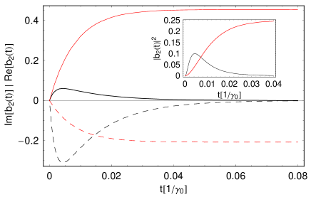
Figure 2: Variations of Re[$b_{2}(t)$] (solid lines), Im[$b_{2}(t)$] (dashed lines), and $\left|b_{2}(t)\right|^{2}$ (inset) as functions of time for $\omega_{0}=0.602\omega_{p}$ (red lines) and $0.748\omega_{p}$ (black lines). In plotting the figure, the inter-dot distance $z_{0}$ is set equal to $0.35(\omega_{p}a/c)$ with radius $R=0.1$.

Application in entanglement generation.–Let us now put another QD close to the wire, the interaction between the wire and QDs can now be written as

$$H^{\prime}=\sum_{n,k_{z}}g_{n,k_{z}}(\sigma_{1+}+\sigma_{2+}e^{ik_{z}z_{0}})\widehat{a}_{n,k_{z}}+h.c.,$$ (7)

where $a_{n,k_{z}}$ is the surface-plasmon operator, $\sigma_{j+}$ is the creation operator of the $j$-th QD. Note that in Eq. (7) we have assumed no detuning and the two dots have the same separation from the metal wire. Since the propagating modes are along the $z$-direction only, the phase difference acquired by the second dot is $ik_{z}z_{0}$, where $z_{0}$ is the separation between the two dots. If one further assumes that only QD-1 is initially excited, the state vector  of the system can be written as

$$\left|\Psi(t)\right\rangle=b_{1}(t)\left|\uparrow\downarrow;0\right\rangle+b_{2}(t)\left|\downarrow\uparrow;0\right\rangle+\sum_{n,k_{z}}b_{n,k_{z}}(t)\left|\downarrow\downarrow;1_{n,k_{z}}\right\rangle$$ (8)

with $b_{1}(0)=1$ and $b_{2}(0)=b_{n,k_{z}}(0)=0$. Here, $\left|\uparrow\downarrow;0\right\rangle$ ($\left|\downarrow\uparrow;0\right\rangle$) means that QD-1(-2) is excited, while $\left|\downarrow\downarrow;1_{n,k_{z}}\right\rangle$ represents that both the QDs are deexcited with the presence of single surface-plasmon. If we let the exciton band-gap $\omega_{0}$ far away from the band-edge, $b_{1}(t)$ and $b_{2}(t)$ can be obtained easily by solving the time-dependent Schrödinger equation.

Fig. 2 shows the time variations of Re[$b_{2}(t)$], Im[$b_{2}(t)$], and $\left|b_{2}(t)\right|^{2}$ for different values of the exciton bandgap. For $\omega_{0}=0.748\omega_{p}$, the population of the second dot vanishes quickly as seen from the black lines. For $\omega_{0}=0.602\omega_{p}$, however, it approaches (quasi-)stationary limit²¹ as shown by the red lines. This is because, for the later case, only $n=0$ mode contributes to the decay rate $\Gamma_{sp}$. In this case, the populations of the dots can be analytically written as

$$\left\{\begin{array}[]{cc}b_{1}(t)=e^{-2\Gamma_{sp}t}(1+e^{2\Gamma_{sp}t})/2,&\\ b_{2}(t)=e^{-ik_{0}z_{0}-2\Gamma_{sp}t}(-1+e^{2\Gamma_{sp}t})/2.&\end{array}\right.$$ (9)

From Eq. (9), one realizes that there is always 50% chance for the two dots to evolve into the state: $\left|\uparrow\downarrow\right\rangle+$ $e^{-ik_{0}z_{0}}\left|\downarrow\uparrow\right\rangle$. It means that, for example, the singlet [triplet] entangled state can be created if $k_{0}z=(2m+1)\pi$ [$2m\pi$] with $m$ being an integer. The advantage is that the entangled states can be generated with a remote sense, such that one can manipulate/control one qubit without affecting another. One should be reminded again such an entanglement is generated from the collective decay (super-radiance) in one dimension²², not from the trivial single-mode Rabi coupling, since the decay rate $\Gamma_{sp}$ is still present in Eq. (9).

In summary, we have shown that radiative decay of colloidal QD excitons into surface plasmons can be greatly enhanced at certain values of the exciton bandgap. The enhancement is due to zero-slope in dispersion relation, and one has to treat the decay dynamics with a non-Markovian way. In addition, an idea of creating remote entangled states between two QDs is also proposed and can be tested with current technology²³.

.1 Acknowledgments

We would like to thank Prof. T. Brandes at Technische Universität Berlin and Dr. J. Taylor at MIT for helpful discussions. This work is supported partially by the National Science Council, Taiwan under the grant numbers NSC 96-2112-M-009-021 and 95-2112-M-006-031-MY3.

References

- (1) R. H. Ritchie, Phys. Rev. 106, 874 (1957); H. A. Atwater, Sci. Am. 296, 56 (2007).
- (2) C. A.Pfeiffer, E. N. Economou and K. L. Ngai, Phys. Rev. B 10, 3038 (1974); S. S. Martinos and E. N. Economou, Phys. Rev. B 28, 3173 (1983); S. S. Martinos, Phys. Rev. B 31, 2029 (1985).
- (3) R. Zia and M. L. Brongersma, Nature Nanotechnology 2, 426 (2007).
- (4) W. L. Barnes, A. Dereux, and T. W. Ebbesen, Nature 424, 824 (2003).
- (5) J. Takahara, S. Yamagishi, H. Taki, A. Morimoto, and T. Kobayashi, Opt. Lett. 22, 475 (1997).
- (6) D. K. Gramotnev, and D. F. P. Pile, Appl. Phys. Lett. 85, 6323 (2004).
- (7) D. F. P. Pile, and D. K. Gramotnev, Opt. Lett. 29, 1069 (2004).
- (8) S. I. Bozhevolnyi, V. S. Volkov, E. Devaux, J. Laluet, and T. W. Ebbesen, Nature 440, 508 (2006).
- (9) D. Pacifici, H. J. Lezec, and H. A. Atwater, Nature Photonics 1, 402 (2007).
- (10) H. F. Arnoldus and T. F. George, Phys. Rev. A 37, 761 (1988).
- (11) A. Neogi, C.-W. Lee, H. O. Everitt, T. Kuroda, A. Tackeuchi, and E. Yablonovitch, Phys. Rev. B 66, 153305 (2002); A. Neogi, and H. Morkoç, Nanotechnology 15, 1252 (2004); A. Neogi, H. Morkoç, T. Kuroda, and A. Tackeuchi, Opt. Lett. 30, 93 (2005).
- (12) P. B. Johnson and R. W. Christy, Phys. Rev. B 6, 4370 (1972); R. Paiella, Appl. Phys. Lett. 87, 111104 (2005).
- (13) D. E. Chang, A. S. Sørensen, P. R. Hemmer, and M. D. Lukin, Phys. Rev. Lett. 97, 053002 (2006).
- (14) D. E. Chang, A. S. Sørensen, E. A. Demler, and M. D. Lukin, Nature Physics 3, 807 (2007).
- (15) I. Gontijo, M. Boroditsky, E. Yablonovitch, S. Keller, U. K. Mishra, and S. P. DenBaars, Phys. Rev. B 60, 11564 (1999).
- (16) G. Schlegel, J. Bohnenberger, I. Potapova, and A. Mews, Phys. Rev. Lett. 88, 137401 (2002).
- (17) C. T. Yuan, W. C. Chou, Y. N. Chen, J. W. Chou, D. S. Chuu, C. A. Lin, J. K. Li, W. H. Chang, and J. L. Shen, J. Phys. Chem. C, 111 (42), 15166 (2007).
- (18) J. A. Stratton, Electromagnetic Theory (McGraw-Hill, New York, 1941).
- (19) From the numerical results, the imaginary parts of for the bound modes are actually very small ( of the real parts).
- (20) Sajeev John and Tran Quang, Phys. Rev. A 50, 1764 (1994); Shi-Yao Zhu, Yaping Yang, Hong Chen, Hang Zheng, and M. S. Zubairy, Phys. Rev. Lett. 84, 2136 (2000).
- (21) In fact, the exciton eventually decays into free space. Since the coupling to the surface plasmons is so strong, one can roughly neglecte the effect from vacuum fluctuations in the regime of .
- (22) Y. N. Chen, D. S. Chuu, and T. Brandes, Phys. Rev. Lett. 90, 166802 (2003).
- (23) A. V. Akimov, A. Mukherjee, C. L. Yu, D. E. Chang, A. S. Zibrov, P. R. Hemmer, H. Park, and M. D. Lukin, Nature 450, 402 (2007).