Fast Wavelet-Based Visual Classification

Abstract

We investigate a biologically motivated approach to fast visual classification, directly inspired by the recent work [20]. Specifically, trading-off biological accuracy for computational efficiency, we explore using wavelet and grouplet-like transforms to parallel the tuning of visual cortex V1 and V2 cells, alternated with max operations to achieve scale and translation invariance. A feature selection procedure is applied during learning to accelerate recognition. We introduce a simple attention-like feedback mechanism, significantly improving recognition and robustness in multiple-object scenes. In experiments, the proposed algorithm achieves or exceeds state-of-the-art success rate on object recognition, texture and satellite image classification, language identification and sound classification.

1 Introduction

Automatic object recognition and image classification are important and challenging tasks. This paper is inspired by the remarkable recent work of Poggio, Serre, and their colleagues [20], on rapid object categorization using a feedforward architecture closely modeled on the human visual system. The main directions it departs from that work are twofold. First, trading-off biological accuracy for computational efficiency, our results exploit more engineering-motivated mathematical tools such as wavelet and grouplet transforms [13, 12], allowing faster computation and limiting ad-hoc parameters. Second, the approach is generalized by adding a degree of feedback (another known component of human perception), yielding significant performance and robustness improvement in multiple-object scenes. In experiments, the resulting scale- and translation-invariant algorithm achieves or exceeds state-of-the-art performance in object recognition, but also in texture and satellite image classification, and in language identification.

2 Algorithm description

2.1 Feature computation and classification

As in [20], the algorithm is hierarchical. In addition, motivated in part by the relative uniformity of cortical anatomy [14, 21], the two layers of the hierarchy are made to be computationally similar, as shown in Fig. 1. Layer one performs a wavelet transform [13] in the $\mathbf{S_{1}}$ unit followed by a local maximum operation in the $\mathbf{C_{1}}$ unit. The transform in the $\mathbf{S_{2}}$ unit in layer two is similar to the grouplet transform [12], and is followed by a global maximum operation in the $\mathbf{C_{2}}$ unit.

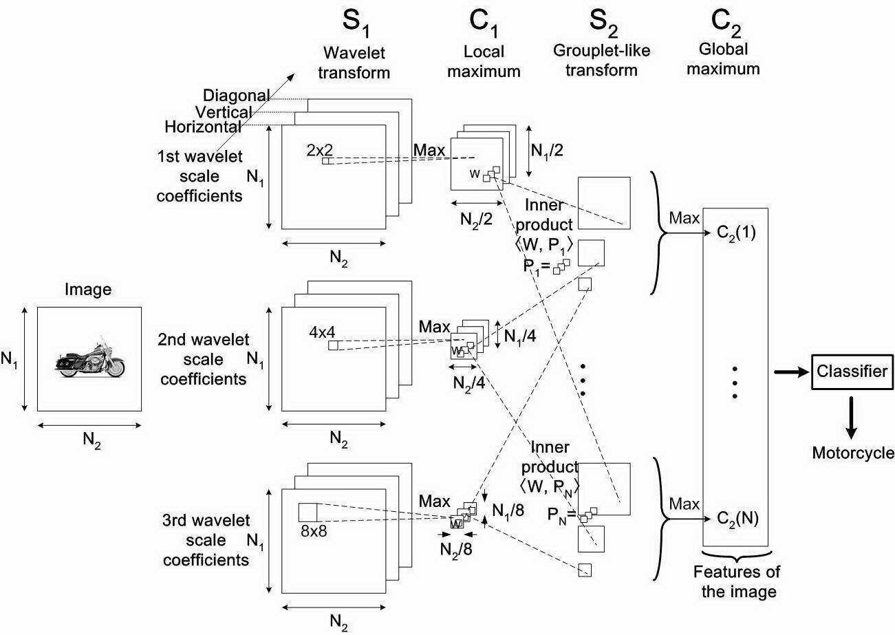
Figure 1: Algorithm overview.

$\mathbf{S_{1}}:$ Wavelet transform. The frequency and orientation tuning of cells in visual cortex V1 can be interpreted as performing a wavelet transform of the retinal image [13]. Let us denote $f(x,y)$ a gray-level image of size $N_{1}\times N_{2}$. A translation-invariant wavelet transform is performed on the image:

$$Wf(u,v,j,k)=\sum_{x=1}^{N_{1}}\sum_{y=1}^{N_{2}}f(x,y)\frac{1}{2^{j}}\psi^{k}\left(\frac{x-u,y-v}{2^{j}}\right),\vspace{-1ex}$$

where $k=1,2,3$ denotes the orientation (horizontal, vertical, diagonal), $\psi^{k}(x,y)$ is a wavelet function and $Wf$ are the wavelet coefficients. Scale invariance is achieved by a normalization

$$S_{1}(u,v,j,k)=\frac{|Wf(u,v,j,k)|}{\|f\|^{2}_{\textrm{supp}(\psi^{k}_{j})}},\vspace{-2ex}$$

where $\|f\|^{2}_{\textrm{supp}(\psi^{k}_{j})}$ is the image energy within the support of the wavelet $\psi^{k}\left(\frac{x-u,y-v}{2^{j}}\right)$. One can verify that

$$S_{1}(u,v,j,k)\sim S_{1}^{\prime}(2^{\beta}u,2^{\beta}v,\beta j,k)\vspace{-2ex}$$

where $S_{1}$ and $S_{1}^{\prime}$ are the coefficients of $f(x,y)$ and of its $2^{\beta}$-time zoomed version $f({x}/{2^{\beta}},{y}/{2^{\beta}})$. The normalization also makes the recognition invariant to global linear illumination change.

$\mathbf{C_{1}}:$ Local maximum Limited translation invariance is achieved at this stage by keeping the local maximum of $S_{1}$ coefficients in a subsampling procedure:

$$C_{1}(u,v,j,k)=\max_{u^{\prime}\in[2^{j}(u-1)+1,2^{j}u),v^{\prime}\in[2^{j}(v-1)+1,2^{j}v)}S_{1}(u^{\prime},v^{\prime},j,k),\vspace{-1ex}$$

the maximum being taken at each scale $j$ and orientation $k$ within a spatial neighborhood of size proportional to $2^{j}\times 2^{j}$. The resulting $C_{1}$ map at scale $j$ and orientation $k$ is thus of size $N_{1}/2^{j}\times N_{2}/2^{j}$.

$\mathbf{S_{2}}:$ Grouplet-like transform. Cells in visual cortex V2 and V4 have larger receptive fields comparing to those in V1 and are tuned to geometrically more complex stimuli such as contours and corners [19]. The geometrical grouplets recently proposed by Mallat [12] imitate this mechanism by grouping and re-transforming the wavelet coefficients.

The procedure in $\mathbf{S_{2}}$ is similar to the grouplet transform. Instead of grouping the wavelet coefficients with a multi-scale geometrically adaptive association field and then re-transforming them with Haar-like functions as in [12], responses of $\mathbf{S_{2}}$ are obtained via inner products between $C_{1}$ coefficients and sliding patch functions of different sizes:

$$S_{2}(u,v,j,i)=\sum_{u^{\prime}=1}^{N_{1}/2^{j}}\sum_{v^{\prime}=1}^{N_{2}/2^{j}}\sum_{k=1}^{3}C_{1}(u^{\prime},v^{\prime},j,k)P_{i}(u^{\prime}-u,v^{\prime}-v,k),\vspace{-1ex}$$

where $P_{i}$ of support size $M_{i}\times M_{i}\times 3$ are patch functions that group the 3 wavelet orientations in a square of size $M_{i}\times M_{i}$.

While the grouplet functions are adaptively chosen to fit the geometry in the image [12], the patch functions $P_{i}$, $i=1,\ldots,N$ are learned with a simple random sampling as in [20]: each patch is extracted at a random scale and a random position from the $C_{1}$ coefficients of a randomly selected training image, the rationale being that patterns that appear with high probability are likely to be learned.

$\mathbf{C_{2}}:$ Global maximum. A global maximum operation in space and in scale is applied on $S_{2}$ and the resulting $C_{2}$ coefficients

$$C_{2}(i)=\max_{u,v,j}S_{2}(u,v,j,i)\vspace{-2ex}$$

are thus invariant to image translation and scale change.

Classification The classification uses $C_{2}$ coefficients as features and thus inherits the translation and scale invariance. While various classifiers such as SVMs can be used, a simple but robust nearest neighbor classifier will be applied in the experiments.

2.2 Feature selection

Structures that appear with a high probability are likely to be learned as patch functions through random sampling. However, they are not necessarily salient and neither are the resulting $C_{2}$ features. This suggests active selection of the learned patches. For example, Lowe and Mutch have constructed sparse patches by retaining one salient direction at each position [18].

A simple patch selection is proposed here by sorting the variances of the $C_{2}$ coefficients of the training images. A small $C_{2}(i)$ variance implies that the corresponding patch $P_{i}$ is not salient. Fig. 2-a plots the variance of the $C_{2}$ coefficients of the motorcycle and the background images in the Caltech5 database (see Fig. 4), the $S_{2}$ patches being learned from the same images. Out of the 1000 patches, 200 salient ones whose resulting $C_{2}$ have non-negligible variance are selected. Other patches usually correspond to nonsalient structures such as a common background and are therefore excluded. Fig. 2-b and c show that after patch selection the 200 $C_{2}$ coefficients are mainly positioned around the object, as opposed to the 1000 $C_{2}$ coefficients spreading over all the image prior to patch selection. The recognition using these salient patches is not only more robust but also 5 times faster.

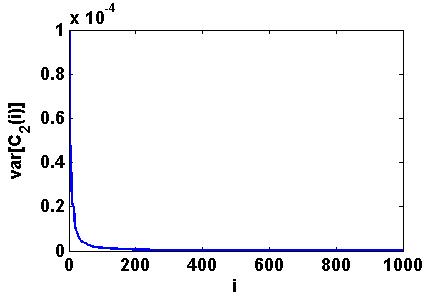
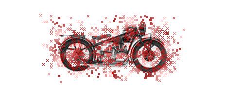
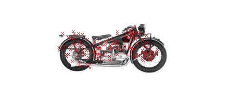
a	b	c

Figure 2: a. Variance of the $C_{2}$ coefficients before patch selection. b and c. Positions of the $C_{2}$ coefficients before and after patch selection (marked by crosses).

2.3 Feedback

Feedback [19, 4, 22] allows tracing back object positions, focusing attention on the objects one by one and thus improving recognition performance in multiple-object scenes.

Object positioning For simplicity the feedback procedure is discussed in a two-object scene but can be applied in the case of multiple objects. $C_{2}$ coefficients are placed around the two objects after selection, as shown in Fig. 3-a. Using a clustering algorithm such as the K-means algorithm, one is able to locate the two objects as illustrated in Fig. 3-b.

Object identification While one could recalculate the features of the attended object cropped out from the whole image, i.e., concentrate all the visual cortex resource on a single object, a faster procedure identifies the attended object, say object $A$, using directly the lower-dimensional feature vector $C_{2A}$, composed of the $C_{2}$ coefficients corresponding to $A$ already calculated in the feedforward pathway. This can be implemented by reclassifying $C_{2A}$ using subsets of the $C_{2}$ coefficients of the training images extracted at the same coordinates of $C_{2A}$, as shown in Fig. 3-c. Discarding the coordinates that are located on the irrelevant object $B$ in the test image disambiguates the classification and improves the recognition of the object $A$.

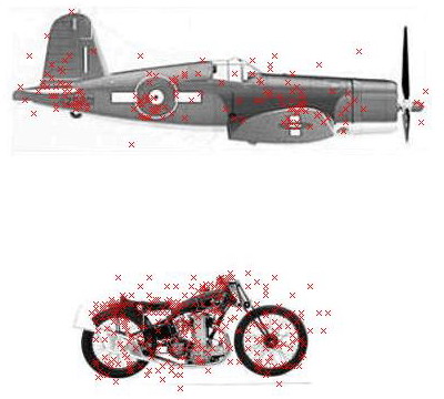
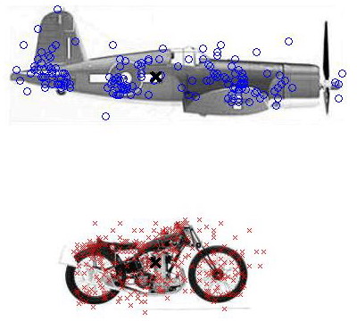
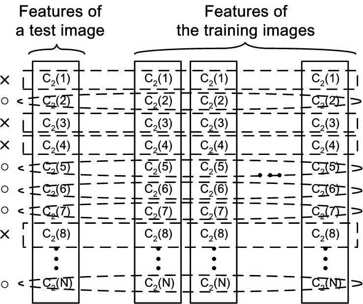
a	b	c

Figure 3: Feedback in a two-object scene. a. Positions of $C_{2}$ coefficients are marked by crosses. b. $C_{2}$ coefficients are clustered (represented by circles vs crosses). c. Feature coefficients of the training images are grouped, the coordinates being in line with the clustering of the coefficients of the test image. Rectangles and ellipses represent the two groups.

3 Experiments

All the experiment results were obtained with the same algorithm configuration. Daubechies 7-9 wavelets of 3 scales were used in $\mathbf{S_{1}}$. In $\mathbf{S_{2}}$ 1000 patches $P_{i}$ of 4 different sizes $M\times M\times 3$ with $M=4,8,12,16$, 250 for each, were learned from the training images. The classifier was the simple nearest neighbor classification algorithm.

For texture and satellite image classification as well as for language identification, one sample image of size $512\times 512$ was available per image class and was segmented to 16 non-overlapping parts of size $128\times 128$. Half were used for training and the rest for test.

3.1 Object recognition

For the object recognition experiments we used 4 data sets that are airplanes, motorcycles, cars (rear) and leaves, plus a background class from the Caltech5 database, some sample images being shown in Fig. 4. The images are turned to gray-level and rescaled in preserving the aspect ratio so that the minimum side length is of 140 pixels. A set of 50 positive images and 50 negative images were used for training and another set for test.

Table 1 summarizes the object recognition. The performance measure reported is the ROC accuracy. Results obtained with the proposed algorithm are superior to previous approaches [2, 24] and comparable to [20] but at a lower computational cost (in Matlab code about 6 times faster with feature selection). Fig. 5-d shows that the performance is improved when the number of $C_{2}$ features increases and is in general stable with 200 features.

Figure 4: Sample images from Caltech5. From left to right: airplanes, motorcycles, cars (rear), leaves and background.

Data sets	Proposed	Serre [20]	Others
Airplanes	96.0	96.7	94.0 [2]
Motorcycles	98.0	98.0	95.0 [2]
Cars (Rear)	96.0	99.8	84.8 [2]
Leaves	92.0	97.0	84.0 [24]

Table 1: Object recognition performance.

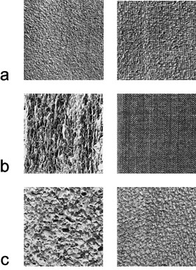
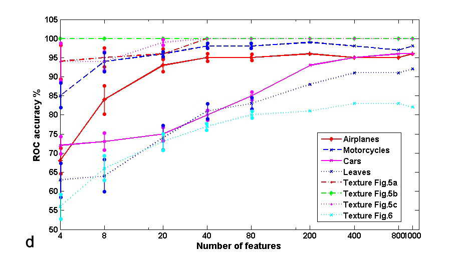
Figure 5: a-c. Pairs of textures. d. Performance vs numbers of $C_{2}$ features.

3.2 Texture classification

Figs. 5-a,b,c and Fig. 6 show respectively 3 pairs of textures that were used for binary classification and a group of 10 textures that were used for multiple-class (10-class) classification, all from the Brodatz database. As summarized in Table 2, the proposed algorithm achieved perfect results for binary classification and for the challenging multiple class classification its performance was comparable to the state-of-the-art methods [8, 6, 17]. Indeed the random patch extraction applied in the algorithm is ideal for classifying stationary patterns such as textures. Fig. 5 shows that stable performance is achieved with as few as 40 features, which confirms the good texture classification results and the robustness of the algorithm.

Figure 6: A group of 10 textures.

Data sets	Proposed	Avg. [17]	Best [17]	Others
Fig. 5-a	100	88.0	99.3	91.5 [6]
Fig. 5-b	100	96.2	99.7	N/A
Fig. 5-c	100	87.6	97.5	88.6 [6]
Fig. 6	82.6	52.6	67.7	83.1 [8]

Table 2: Texture classification performance. From left to right: proposed method, average and best performance of the algorithms summarized in [17], other methods. N/A means that the results were not shown.

Classifying the whole Brodatz database (111 textures) is a more challenging task. Combining $C_{2}$ coefficients with the histogram of the wavelet approximation coefficients as features, the proposed algorithm achieved 87.8% accuracy for the 111-texture classification, comparable to the 88.2% accuracy rate reported in [7] obtained with a state-of-the-art texture classification approach.

3.3 Satellite image classification

Fig. 7 displays 4 classes of satellite images at 0.5 $m$ resolution: urban areas, rural areas, forests and sea. Since access to images at other resolutions is restricted, we simulated the images at resolutions 1 $m$ and 2 $m$ by Gaussian convolution and sub-sampling.

The first experiment tested the multi-class classification of mono-resolution images shown in Fig. 7. 100% classification accuracy was achieved for images of all the 4 classes. The second experiment validated the scale invariance of the proposed algorithm. Images at resolution 0.5 $m$ were used to train the classifier while the classification was tested on images at resolutions 1 $m$ and 2 $m$. Again the classification accuracy was 100%, same as reported in a recent work [11] and significantly higher than earlier methods [5] referenced therein. In addition, image resolution is assumed to be known in [11], whereas the proposed algorithm does not need this information, thanks to its scale invariance.

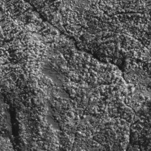
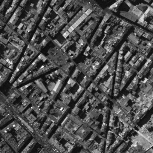
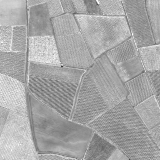
Figure 7: Satellite images. From left to right: forest, urban areas, rural areas, sea.

3.4 Language identification

Language identification aims to determine the underlying language of a document in an imaged format, and is often carried out as a preprocessing of optical character recognition (OCR). Based on principles totally different from traditional approaches [10], the proposed algorithm achieved 100% success rate in a 8-language identification task, as shown in Fig 8.

Figure 8: From top to bottom, left to right: document texts in Arabic, Chinese, English, Greek, Hebrew, Japanese, Korean, Russian.

3.5 Sound Classification

The main idea is to directly extend the above algorithm to sound applications is to view time-frequency representations of sound as textures. Preliminary experiments suggest this may be a fruitful direction of research.

Fig. 9 illustrates 5 types of sounds and samples of their log-spectrograms. 2 minutes excerpts of each sound were collected. The spectrograms were segmented (in time) into segments of 5 seconds. Half were used for training and the rest for test. A direct application of the proposed algorithm using the spectrograms as the visual patterns resulted in 100% accuracy in the 5-sound classification.

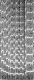
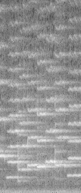
Figure 9: From left to right: violin, piano, trumpet, flute, speech. The figures in the second row are spectrograms of the sounds illustrated in the first row.

3.6 Feedback: multiple-object scenes

Recognition performance tends to degrade when multiple stimuli are presented in the receptive field. Fig. 10-a shows an example of a multiple-object scene in which one searched an object, say an airplane, through a binary classification against a background image. Due to the perturbation from the coexisting stimuli, the feedforward recognition accuracy is as low as 74%. The feedback procedure introduced in Subsection 2.3 improves considerably the accuracy to 98% by focusing attention on each object in turn.

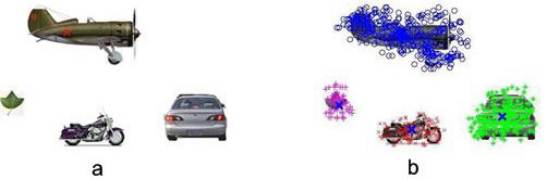
Figure 10: a. A 4-object scene. b. $C_{2}$ coefficients clustering.

4 Conclusion and future work

Inspired by the biologically motivated work of [20], we have described a wavelet-based algorithm which can compete with the state-of-the-art methods for fast and robust object recognition, texture and satellite image classification, language recognition and sound classification. A feedback procedure has been introduced to improve recognition performance in multiple-object scenes.

Potential applications also include video archiving (semantic video analysis), video surveillance, high-throughput drug development, texture retrieval, and robotic learning by imitation.

To further improve and extend the algorithm, a key aspect will be a more refined use of feedback between different levels. Such feedback will naturally involve stability and convergence questions, which will in turn both guide the design of the algorithm and shape its performance. In addition, contrary to the nervous system, the algorithm need not be constrained by information transmission delays between different levels. Preliminary ideas in this direction are briefly discussed in the appendix.

Acknowledgements: We are grateful to Tomaso Poggio and Thomas Serre for many discussions about their recognition system, to Stéphane Mallat for stimulating discussions on wavelets and grouplets and to Jean-Michel Morel for important discussions on invariant image recognition.

APPENDIX

Appendix A Dynamic System Perspective

A.0.1 Basic algorithm

The first step towards introducing a dynamic systems perspective aimed at further development of feedback mechanisms is simply to rewrite the algorithm in terms of differential equations, which puts it in a form more suitable to subsequent analysis of stability and convergence.

Let ${{\mathbf{x}}_{1}}$ be the output of the $S_{1}/C_{1}$ layer, and ${{\mathbf{x}}_{2}}$ be the output of the $S_{2}/C_{2}$ layer (in our static implementation above, we simply have ${{\mathbf{x}}_{1}}=C_{1}$ and ${{\mathbf{x}}_{2}}=C_{2}$).

For a single object, the basic algorithm can be trivially computed by a dynamic system of the form

$\dot{{\mathbf{x}}}_{1}=-k_{1}({{\mathbf{x}}}_{1}-C_{1})$

$\dot{{\mathbf{x}}}_{2}=-k_{2}({{\mathbf{x}}}_{2}-C_{2})$

For multiple objects, the clustering process described in section 2.3 can be implemented by introducing a scalar state ${x_{3}}$, which spikes for each object in sequence

$\dot{x}_{3}=\rho(x_{3},C_{2})$

with spike amplitude equal to $1$ $-$ the function $\rho(x_{3},C_{2})$ is discussed later in this section and in a companion paper. The dynamics of ${{\mathbf{x}}}_{2}$ can be modified in turn so that states corresponding to each object appear in sequence according to the state $x_{3}$

$\dot{{\mathbf{x}}}_{1}=-k_{1}({{\mathbf{x}}}_{1}-C_{1})$

$\dot{{\mathbf{x}}}_{2}=-k_{2}({{\mathbf{x}}}_{2}-x_{3}\ {\mathbf{k}}(C_{2A}))$

$\dot{x}_{3}=\rho(x_{3},C_{2})$

where, componentwise, ${\mathbf{k}}(C_{2A})=C_{2A}$ where $C_{2A}$ is active and and ${\mathbf{k}}(C_{2A})=0$ otherwise. Note that $x_{3}$ smoothly transitions between $0$ and $1$ according to the attended object. The positive gain $k_{2}$ is chosen such that $k_{2}T\gg 1$, where $T$ is the spike duration, itself a fraction of the interspike period.

The above equations simply implement the basic algorithm and display objects in sequence, without introducing any new feature at this point.

Techniques for globally stable spike-based clustering are described in a companion paper, based on modified FitzHugh-Nagumo neural oscillators [3, 15], similar to [1],

$$\dot{v}_{i} = 3v_{i}-v_{i}^{3}-v_{i}^{7}+2-w_{i}+I_{i}$$ (1)

$$\dot{w}_{i} = c[\alpha(1+\tanh(\beta v_{i}))-w_{i}]$$

where $v_{i}$ is the membrane potential of the oscillator, $w_{i}$ is an internal state variable representing gate voltage, $I_{i}$ represents the external current input, and $\alpha$, $\beta$ and $c$ are strictly positive constants. Using a diagonal metric transformation ${\mathbf{\Theta}}={\rm diag}(\sqrt{c\alpha\beta},1)$, one easily shows, similarly to [23], that

$${\mathbf{\Theta}}{\mathbf{J}}{\mathbf{\Theta}}^{-1}\ <\ {\rm diag}(\ 3+\frac{\alpha\beta}{4}\ ,\ 0\ )$$

where ${\mathbf{J}}$ is the Jacobian matrix of $(\ref{FN_sat})$, leading to simple global stability conditions based on [16] (section 2.2).

A.1 Generalized diffusive connections

One of the most immediate additional feedback mechanisms to be explored is that of generalized diffusive connections ([16], section 3.1.2). In a feedback hierarchy, these correspond to achieving consensus between multiple processes of different dimensions.

A.2 Tracking of time-varying images

Similarly to [9], composite variables for dynamic tracking can be used at every level, based on both top-down an bottom-up information. This allows one to implicitly introduce time-derivatives of signals in the differential equations, without having to measure or compute these terms explicitly.

References

- [1] K. Chen and D.L. Wang, “A dynamically coupled neural oscillator network for image segmentation.”, Neural Networks, vol. 15, 423-439.
- [2] R. Fergus and P. Perona and A. Zisserman, “Object class recognition by unsupervised scale-invariant learning”, CVRP, vol.2, pp.264-271, 2003.
- [3] R. FitzHugh, “Impulses and physiological states in theoretical models of nerve membrane”, Biophysical Journal, vol.1, pp.445-466, 1961.
- [4] J. Hawkins, S.Blakeslee, On Intelligence, Times Books, 2004.
- [5] R.M.Haralick, K.Shanmugam, I.Dinstein, “Textural Features for Image Classification”, IEEE Trans. on Sys Man Cy, SMC-3, (6): 610-621, 1973.
- [6] K. Kim, K. Jung, S. Park, and H. Kim, “Support Vector Machines for Texture Classification”, IEEE Trans. PAMI, vol.24, no.11, pp.1542-1550, 2002.
- [7] S. Lazebnik, C. Schmid and J. Ponce, “A Sparse Texture Representation Using Local Affine Regions”, IEEE Transactions on Pattern Analysis and Machine Intelligence, vol. 27, no. 8, pp. 1265-1278, 2005.
- [8] X. Liu and D. Wang, “Texture classification using spectral histograms”, IEEE Trans. PAMI, vol.12, pp.661-670, 2003.
- [9] W. Lohmiller, and J.J.E. Slotine, “Global Convergence Rates of Nonlinear Diffusion for Time-Varying images”, Scale-Space Theories in Computer Vision, Lecture Notes in Computer Science, vol.1682, Springer Verlag (1999).
- [10] S. Lu and C. Tan, “Script and Language Identification in Noisy and Degraded Document Images”, IEEE Trans. PAMI, vol.30, no.1 pp.14-24, 2008.
- [11] B.Luo, J-F.Aujol, Y.Gousseau, S.Ladjal, “Indexing of satellite images with different resolutions by wavelet features”, IEEE Trans Image Proc, accepted, 2008.
- [12] S. Mallat, “Geometrical Grouplets”, ACHA, to appear, 2008.
- [13] S. Mallat, A Wavelet Tour of Signal Processing, Academic Press, 2nd edition, 1999.
- [14] V. Mountcastle, “An Organizing Principle for Cerebral Function: The Unit Model and the Distributed System”, The Mindful Brain, MIT Press, 1978.
- [15] J. Nagumo. and S. Arimoto, and S. Yoshizawa, “An Active Pulse Transmission Line Simulating Nerve Axon,” Proceedings of the IRE, 50(10), pp.2061-2070,1962.
- [16] Q.C. Pham and J.J.E. Slotine, “Stable Concurrent Synchronization in Dynamic System Networks,” Neural Networks, 20(1), 2007.
- [17] T. Randen and J. Husoy, “Filtering for Texture Classification: A Comparative Study”, IEEE Trans on Image Proc, vol.21, no.4, pp.291-310, 1999.
- [18] J. Mutch and D. Lowe, “Multiclass Object Recognition with Sparse, Localized Features”, CVPR 06, pp.11-18.
- [19] R.P.N. Rao and D.H. Ballard, “Predictive coding in the visual cortex: A functional interpretation of some extra-classical receptive-field effects”, Nature Neuroscience, 2, 1, 79, 1999.
- [20] T. Serre, L. Wolf, S. Bileschi, M. Riesenhuber and T. Poggio, “Robust Object Recognition with Cortex-Like Mechanisms”, IEEE Trans. PAMI, vol.29, no.3, pp.411-426, 2007.
- [21] Von Melchner, L., Pallas, S.L. and Sur, M, “Visual behavior mediated by retinal projections directed to the auditory pathway”, Nature, 404, 2000.
- [22] D. Walther, T. Serre, T. Poggio and C. Koch, “Modeling feature sharing between object detection and top-down attention”, VSS, May 2005.
- [23] W. Wang and J.J.E. Slotine, “On Partial Contraction Analysis for Coupled Nonlinear Oscillators,” Biological Cybernetics, 92(1), 2005.
- [24] M. Weber and M. Welling and P. Perona, “Unsupervised Learning of Models for Recognition”, ECCV, pp.18-32, 2000.
- [25]