Prospects and Pitfalls of Gravitational Lensing in Large Supernova Surveys

Abstract

Aims. To investigate the effect of gravitational lensing of supernovae in large ongoing surveys.

Methods. We simulate the effect of gravitational lensing magnification on individual supernovae using observational data input from two large supernova surveys. To estimate the magnification due to matter in the foreground, we simulate galaxy catalogs and compute the magnification along individual lines of sight using the multiple lens plane algorithm. The dark matter haloes of the galaxies are modelled as gravitational lenses using singular isothermal sphere or Navarro-Frenk-White profiles. Scaling laws between luminosity and mass, provided by Faber-Jackson and Tully-Fisher relations, are used to estimate the masses of the haloes.

Results. While our simulations show that the SDSSII supernova survey is marginally affected by gravitational lensing, we find that the effect will be measurable in the SNLS survey that probes higher redshifts. Our simulations show that the probability to measure a significant ($3\sigma$) correlation between the Hubble diagram residuals and the calculated lensing magnification is $\ga 95\%$ in the SNLS data. Moreover, with this data it should be possible to constrain the normalisation of the masses of the lensing galaxy haloes at the $1\sigma$ and $2\sigma$ confidence level with $\sim 30\%$ and $\sim 60\%$ accuracy, respectively.

1 Introduction

Type Ia supernovae (hereafter SNe Ia) are exceptionally useful tools for cosmological investigations. Ongoing large supernova surveys, such as ESSENCE (Miknaitis et al. 2007; Wood-Vasey et al. 2007), SNLS (Astier et al. 2006) and SDSSII (Frieman et al. 2008) harvest hundreds of distant supernovae with high precision.

Several effects will alter the luminosity of these distant sources, and thus dilute the cosmological signal. In this paper we investigate gravitational lensing (de)magnification of the light from these explosions. Although this effect is hardly large enough to dominate the uncertainties in current experiments, as has already been addressed by several groups on statistical grounds (e.g., Riess et al. 2004; Holz & Linder 2005; Astier et al. 2006; Wood-Vasey et al. 2007), the question if it can be corrected for on an individual supernova basis remains. This has been investigated in a series of papers (Gunnarsson et al. 2006; Jönsson et al. 2006) and a tentative detection of a correlation between calculated lensing magnification and Hubble residuals was recently found using the very high-$z$ supernovae in the GOODS field (Jönsson et al. 2007).

In this paper we investigate to what extent other surveys can be affected. The GOODS supernovae (Riess et al. 2004; Strolger et al. 2004; Riess et al. 2007) remain unique in that their large distances clearly make them more likely to be lensed. On the other hand, the ongoing ground based surveys will measure significantly more supernovae with much better sampling, and the improved statistics may well compensate for the smaller distances. To find out which surveys are most likely to display a lensing signal we have performed simulations based on our previous work. The results are presented below, and show that the prospects of detecting lensing are very good.

In Sect. 2 we briefly introduce the surveys we have investigated and the data from these surveys that are used as input for the simulations. A short summary of gravitational lensing of SNe Ia is given in Sect. 3. Section 4 describes the simulations and the results are presented in Sect. 5, where we also discuss how a detection of a lensing signal could be used to obtain information about the lensing matter. Finally, we summarise our results in Sect. 6.

2 Supernova surveys

There are (at least) three ongoing major ground based supernova surveys as mentioned above. We have chosen to simulate the SNLS survey to estimate the effects in a deep survey. It probes a similar redshift range as the ESSENCE survey and is likely to find more supernovae. It is also of importance that SNLS uses several filters which allows photo-$z$ determinations for the field galaxies. The SDSSII supernova survey is selected to investigate if any gravitational lensing effects could be expected for this smaller redshift domain when we have good statistics.

2.1 SNLS

The Supernova Legacy Survey, (SNLS, Astier et al. 2006) has published constraints on the cosmological parameters using 71 SNe Ia ranging from $z=0.2-1.0$ discovered during the first year. Around 500 spectroscopically identified SNe Ia are expected to end up in the final Hubble diagram at the end of the survey. The survey consists of an imaging survey detecting and monitoring the light curves of the SNe, and a spectroscopic follow-up confirming the nature of the SNe and measuring their redshifts. A wide field imager used in ”rolling search” mode allows to perform the discovery and photometric follow-up at the same time. The SNLS is searching for SNe in 4 different fields of 1 square degree each and each field is observed every third to fourth night for as long as it remains visible. Observations are taken in 4 filters (the MegaCam filter set) giving rise to a promising data set for observing the lensing signal.

Since the line of sight to SNe Ia located close to the edge of the fields can not be modelled for gravitational lensing accurately, we estimate that only $\sim 450$ of the $\sim 500$ Hubble diagram SNe Ia can be used to search for a gravitational lensing signal. The parameters from this survey that are needed as input for this investigation (see Gunnarsson et al. 2006) have been taken from the literature (Ilbert et al. 2006) and from discussions with the involved astronomers.

2.2 SDSSII

The Sloan Digital Sky Survey II Supernova Survey (SDSSIISN, Frieman et al. 2008) is searching a 280 square degree field over 3 seasons. The survey is well on track to discover over 500 Type Ia supernovae, of which $\sim 300$ will likely end up in the Hubble diagram. The SDSSII is a follow-up on the previous successfull SDSS projects, which means that this search has a working infrastructure capable of handling large amounts of data. The search is performed in 5 bands ($ugriz$) and the SDSS field is calibrated down to an accuracy of $\sim 1\%$ (Ivezić et al. 2007).

3 Gravitational lensing of SNe Ia

Here we give a short introduction to the aspects of gravitational lensing of SNe Ia which are relevant to this work. For a more thorough introduction to the subject see e.g. Bergström et al. (2000).

Matter inhomogeneities in the Universe give rise to gravitational fields which will influence the path of light rays propagating between a source and an observer. In the weak lensing regime, gravitational bending of light, or gravitational lensing, can lead to changes in the apparent position of the source as well as changes in the flux. For point sources such as SNe Ia, the amplification (or de-amplification) of the flux can be described by the magnification factor, $\mu$. The observed flux from a point source in an inhomogeneous universe is given by $f_{\rm obs}=\mu f$, where $f$ is the flux that would be observed in a homogeneous universe in the absence of lensing. Amplification and de-amplification relative to a homogeneous universe is consequently described by $\mu>1$ and $\mu<1$, respectively.

The distribution of magnification factors, $P(\mu)$, for sources at a specific redshift depends on the distribution of matter between the source and the observer. In general $P(\mu)$ is asymmetric with a peak at $\mu<1$ and a high magnification tail. Due to flux conservation, as long as we do not have multiple images, the average magnification is unity, i.e. $\langle\mu\rangle=\int P(\mu)\mu d\mu=1$. The average flux from a number of standard candles, all at the same redshift, $\langle f_{\rm obs}\rangle=\langle\mu\rangle f=f$, is thus an unbiased distance indicator if the variance of the flux is finite. However, changes in the flux from standard candles will increase the dispersion in distance measurements and could potentially lead to selection effects.

4 Simulations

We use simulations to investigate the effects of gravitational lensing for the surveys described in Sect. 2. Since gravitational lensing depends on the distribution of matter between the source and the observer, a model of the matter distribution is needed in order to simulate gravitational magnification. In the next section we briefly describe our model of the matter distribution in the Universe, which is based on observational input. For more details we refer the reader to Gunnarsson et al. (2006) where our model is described in detail.

4.1 Simulating lines of sight

For each simulated SN Ia we simulate a line of sight populated by foreground galaxies. The galaxy population is characterised by the luminosity functions presented in Dahlén et al. (2005). These luminosity functions are used to simulate the number of galaxies along a line of sight as well as their brightness and type. Simulated $B$-band absolute magnitudes of the galaxies are in the range $-23<M_{B}<-16$. A constant comoving number density of galaxies with redshift is assumed. Since the position of the galaxies in the sky as well as the redshifts are assigned at random, clustering of matter into larger structures is not taken into account.

Each galaxy is associated with a dark matter halo and we assume that the mass of the halo can be obtained from the luminosity of the galaxy. Gravitational lensing depends not only on the mass of the lens, but also on the distribution of matter within the lens. We will model the galaxy haloes using singular isothermal sphere (SIS) and Navarro-Frenk-White (NFW, Navarro et al. 1997) profiles. Since these profiles are divergent, they are truncated at $r_{200}$, the radius inside which the mean density is 200 times the critical density of the Universe. We use numerical routines (Navarro et al. 1997) to find the concentration of a halo characterised by the mass $m_{200}$ enclosed within the radius $r_{200}$.

To convert galaxy luminosity to halo mass we relate dynamical properties of the galaxies to the dark matter halo. For a SIS halo, $m_{200}$ is related to the velocity dispersion, $\sigma$, via the formula

$$m_{200}=\frac{\sqrt{2}\sigma^{3}}{5GH_{0}}.$$ (1)

This formula is a good approximation also for a NFW halo with the same corresponding maximum rotation velocity, $V_{\rm max}$. The mass of a NFW halo is over-estimated by $5-15\%$ when Eq. (1) is used to calculate $m_{200}$ for a given value of $V_{\rm max}$. The velocity dispersion of early type galaxies can be obtained from the absolute magnitudes through the Faber-Jackson (F-J) relation as derived by Mitchell et al. (2005)

$$\log\sigma=-0.091(M_{B}-4.74+0.85z).$$ (2)

The redshift dependence in the relation accounts for the brightening of the stellar population with redshift. We represent the measurement error in this relation by the scatter in the SDSS measurements reported by Sheth et al. (2003)

$${\rm rms}(\log\sigma)=0.079[1+0.17(M_{B}+19.705+0.85z)].$$ (3)

For late type galaxies we use the Tully-Fisher (T-F) relation derived by Pierce & Tully (1992), with correction for redshift calculated by Böhm et al. (2004),

$$\log V_{\rm max}=-0.134(M_{B}+3.61+1.22z),$$ (4)

to relate galaxy luminosity to the maximum rotation velocity of the galaxy. The velocity dispersion relates to the maximum rotation velocity via $\sigma=V_{\rm max}/\sqrt{2}$. For the T-F relation the observed scatter is ${\rm rms}(M_{B})=0.41$, which corresponds to

$${\rm rms}(\log V_{\rm max})=0.06.$$ (5)

The mass range for early and late type galaxies computed using the formulae above is $4\times 10^{11}<m_{200}/M_{\sun}<3\times 10^{13}$ and $3\times 10^{10}<m_{200}/M_{\sun}<2\times 10^{13}$, respectively.

The code used to compute the magnification factor for the simulated lines of sight is described in the following subsection.

4.2 Q-LET

The Quick Lensing Estimation Tool (Q-LET, Gunnarsson 2004) is a numerical code which utilises the multiple lens plane algorithm. Each dark matter halo is projected into a lens plane perpendicular to the line of sight situated at the angular diameter distance corresponding to the redshift of the galaxy. The deflection angle is then computed for each lens plane and a ray originating at the position of the image is traced back to the source position via the lens equation. From the Jacobian determinant of the lens equation, the magnification factor can be computed.

In our model universe, the matter density of dark matter galaxy haloes, $\rho_{\rm g}(z)$, is typically less than the measured global matter density $\rho_{\rm m}(z)=\Omega_{\rm M}\rho_{\rm c}^{0}(1+z)^{3}$, where $\rho_{\rm c}^{0}$ is the present critical density of the Universe. Since only galaxies brighter than the magnitude limit will be associated with haloes, we expect $\rho_{\rm g}(z)$ to decrease with redshift. To ensure that our model is consistent, we describe the matter which is “missing” due to our ignorance as a smoothly distributed component characterised by the smoothness parameter given by $\eta(z)=1-\rho_{\rm g}(z)/\rho_{\rm m}(z)$.

Numerical routines in Kayser et al. (1997), which can handle a redshift dependent smoothness parameter, are used to calculate the angular diameter distances in a clumpy universe which are involved in the gravitational lensing calculations.

4.3 Estimating magnification factors

It should be possible to detect gravitational lensing of SNe Ia through the expected correlation between $f_{\rm obs}$ and $\mu$. However, since $\mu$ is not observable we have to use an estimate, $\mu_{\rm est}$, when we search for the correlation. To simulate the precision to which magnification factors can be estimated, we first compute $\mu$ for a fiducial model and then try to recover the value of the magnification factor in the presence of different uncertainties. These uncertainties, which are described in the following paragraphs, dilutes the lensing signal carried by the estimated magnification factor $\mu_{\rm est}$.

Finite field size

Only a limited number of foreground galaxies can be taken into account in the calculations, since the fields are of finite size. To limit this source of error to the percent level, all galaxies within $60\arcsec$ should be included (Gunnarsson et al. 2006). To include this source of error in our simulations a larger number of galaxies is included in the calculation of $\mu$ (all galaxies within $100\arcsec$) than in the calculation of $\mu_{\rm est}$ (all galaxies within $60\arcsec$).

Photometric redshifts

Only galaxies brighter than the magnitude limit can be included in our calculations of the estimated magnification factors, $\mu_{\rm est}$. For surveys like SNLS we have to rely upon photometric redshifts in our calculations. The magnitude limit of the SNLS is $i^{\prime}_{\rm AB}=25.5$, but reliable photometric redshifts can only be obtained to $i^{\prime}_{\rm AB}=24$, which we take as the magnitude limit in our simulations. Photometric redshifts, $z_{\rm p}$, usually have larger uncertainties than spectroscopic redshifts, $z_{\rm s}$. More accurate photometric redshifts can be obtained for bright galaxies than for faint galaxies. According to Ilbert et al. (2006) the photometric redshift accuracy of galaxies observed within the CFHT legacy survey with brightness $17.5<i^{\prime}_{\rm AB}<22.5$ and $22.5<i^{\prime}_{\rm AB}<24$ is $\sigma_{\Delta z/(1+z)}=0.029$ and $\sigma_{\Delta z/(1+z)}=0.034$, respectively.

For some fraction, $f$, of the galaxies, the calculation of the photometric redshift fails miserably. These erroneous - or “catastrophic” - redshifts often arise due to confusion between the Lyman break ($\lambda_{\rm L}=1215$ Å) and the Balmer break ($\lambda_{\rm B}=4000$ Å). We use a simple model of catastrophic redshifts based on this confusion and the results presented in Ilbert et al. (2006). When the Lyman and Balmer breaks are confused either the condition

$$(1+z_{\rm p})\lambda_{\rm B}=(1+z_{\rm s})\lambda_{\rm L},$$ (6)

or the condition

$$(1+z_{\rm p})\lambda_{\rm L}=(1+z_{\rm s})\lambda_{\rm B},$$ (7)

is fulfilled. If the condition expressed by Eq. (6) is fulfilled, the photometric redshift is under-estimated. This condition can only be fulfilled if $z_{\rm s}>2.3$. On the other hand, the photometric redshift is over-estimated if Eq. (7) is fulfilled. According to Fig. 6c in Ilbert et al. (2006) over-estimation of $z_{\rm p}$ is $\sim 5$ times more frequent than under-estimation. In our simple model a fraction $f=1.9\%$ (Ilbert et al. 2006) of the bright galaxies ($17.5<i^{\prime}_{\rm AB}<22.5$) are assigned catastrophic redshifts. The proportion of catastrophic redshifts computed using Eq. (6) and Eq. (7) is 1:5. For the faint galaxies ($22.5<i^{\prime}_{\rm AB}<24$) we use the same model, but the fraction of catastrophic redshifts is higher, $f=5.5\%$ (Ilbert et al. 2006).

Scatter in the F-J and T-F relations

In the conversion between galaxy luminosity and halo mass, the Faber-Jackson and Tully-Fisher relations are used. The scatter in these relations, given by Eq. (3) and Eq. (5), are the largest sources of uncertainty in the calculations. When $\mu_{\rm est}$ is estimated this scatter is taken into account. We also investigate the effects of systematic errors in the relations between luminosity and mass (see Sect. 5.5). Missclassification of galaxy type is a related potential uncertainty which we have not investigated. However, since the missclassification rate for the brightest galaxies, which are also the most important lenses, is likely (Dahlén 2008) to be only a few percent, we assume the neglection of this source of uncertainty to be safe.

Halo models

For the fiducial model, all galaxies are described by NFW profiles. When we estimate the uncertainties in the magnification factor we assume incorrect halo models, i.e. SIS instead of NFW profiles, for 50% of the lenses.

4.4 Correlation

To predict the probability of detecting a correlation between estimated magnifications and Hubble diagram residuals we use Monte Carlo simulations. A large number of SNe Ia data sets are simulated and for each data set the linear correlation coefficient, $r$, is computed. The residuals in the Hubble diagram, which is built of SNe Ia corrected for light curve shape and color, depends on the true magnification factor (computed using the fiducial model),

$$\Delta=-2.5\log_{10}\mu.$$ (8)

In our simulations we add gaussian noise to the Hubble diagram residuals from intrinsic brightness scatter and measurement errors. For the intrinsic dispersion we use the value derived by Astier et al. (2006), $\sigma_{\rm int}=0.13$ mag. To model the measurement errors in the SNLS we use the following redshift dependent fit to the measurement errors in Astier et al. (2006)

$$\sigma_{\rm err}=\left\{\begin{array}[]{ll}0.05\mbox{ mag}&\mbox{ if $z<0.8$}\\ 0.84z^{2}-1.04z+0.34\mbox{ mag}&\mbox{ if $z\geq 0.8$}.\end{array}\right.$$ (9)

The total noise in the residuals are given by $\sigma_{\rm int}$ and $\sigma_{\rm err}$ added in quadrature. This noise or other sources of noise could in reality be non-gaussian. Such non-gaussianity will be a concern for techniques that try to detect gravitational lensing of SNe Ia based on the asymmetry of the distribution of residuals (e.g., Wang 2005). However, for this study where we calculate the magnification for each individual supernova, as long as the contributions to the residuals are not correlated with the foreground matter, the gravitational lensing signal should not be systematically distorted, only diluted.

The magnification, in logarithmic units, on the other hand, depends on the estimated magnification factor,

$$\Delta_{\mu}=-2.5\log_{10}\mu_{\rm est}.$$ (10)

The uncertainties contributing to the noise in the estimated magnification factors were described in Sect. 4.3.

Since we assume the intrinsic brightness scatter and measurement errors to be gaussian and these errors dominate, the distributions of correlation coefficients are gaussian as well and can be described by the mean value, $\langle r\rangle$, and the standard deviation, $\sigma_{r}$. To evaluate the confidence level of the detection of the correlation, we compare with what we could expect to measure if there is no correlation. For each simulated data set we compute the correlation coefficient of the null hypothesis, $r_{\rm null}$, i.e. the hypothesis of no lensing. Since both distributions are gaussian, the probability of a $n\sigma$ detection is given by

$$P(n\sigma)=\frac{1}{2}{\rm erfc}\left(\frac{\langle r_{\rm null}\rangle+n\sigma_{r_{\rm null}}-\langle r\rangle}{\sqrt{2}\sigma_{r}}\right),$$ (11)

where $\langle r_{\rm null}\rangle$ and $\sigma_{r_{\rm null}}$ refers to the mean and standard deviation of the distribution of $r_{\rm null}$, respectively.

5 Results

5.1 Gravitational magnification

In this section we present some basic properties of the simulated gravitational magnification distributions.

5.1.1 SNLS

We have simulated the magnification distribution for sources following the redshift distribution of the first year SNLS SNe Ia (Astier et al. 2006). The magnification factors used to build up this composite distribution were drawn from redshift dependent magnification distributions, which were all normalised to fulfil the condition $\langle\mu\rangle=1$. Although the average magnification factor is unity, the average value of $\Delta$, which depends on the higher moments of the magnification distribution, deviates from zero, $\langle\Delta\rangle=0.0011$ mag. Of importance is also the median of the magnification distribution, $\Delta_{1/2}=0.0084$ mag, which tells us that most SNe Ia in the SNLS data set are slightly demagnified, and would consequently appear to be more distant than they really are.

5.1.2 SDSSII

According to our simulations, the average and the median of the composite magnification distribution corresponding to the SDSSII SN Ia survey is $\langle\Delta\rangle=0.00018$ mag and $\Delta_{1/2}=0.00080$ mag, respectively. The magnification of most SNe Ia are thus clearly negligible for the SDSSII, which is of course a consequence of the shallower redshifts probed by this survey. Since the expected effect of gravitational lensing is very small for the SDSSIISN, we focus on gravitational lensing of SNLS SNe Ia for the rest of this paper.

5.2 Shifts in cosmological parameters

Gravitational lensing can potentially lead to biased cosmological results. Here we investigate and quantify these effects for the SNLS and show that the effects are indeed rather small. We have studied shifts in cosmological parameters for two cases:

1. The universe is assumed to be flat and dominated by a cosmological constant. In this case the present matter density, $\Omega_{\rm M}$ is fitted to simulated data sets.

2. The universe is assumed to be flat and the dark energy equation of state parameter, $w$, is furthermore assumed to be constant. In this case $\Omega_{\rm M}$ and $w$ are simultaneously fitted to data and constrains from Baryonic Acoustic Oscillations (BAO, Eisenstein et al. 2005) are used.

A simulated low redshift data set consisting of 44 SNe Ia, with properties similar to that used by Astier et al. (2006), is used to anchor the Hubble diagram.

We characterise the shift in $\Omega_{\rm M}$ and $w$ by the differences, $\Delta\Omega_{\rm M}=\Omega_{\rm M}^{\rm lensed}-\Omega_{\rm M}$ and $\Delta w=w^{\rm lensed}-w$, in the best fit values obtained with and without gravitational lensing. Our results are collected in Table 1.

Table 1: Average and root mean square of distributions of $\Delta\Omega_{\rm M}$ and $\Delta w$ for case 1 and case 2 for different SNLS like data sets with and without bright outliers removed.

	Outliers	Case 1		Case 2
$N$	removed	$\langle\Delta\Omega_{\rm M}\rangle$	$\sigma_{\Delta\Omega_{\rm M}}$	$\langle\Delta w\rangle$	$\sigma_{\Delta w}$
70	no	$-0.0013$	$0.0075$	$-0.0020$	$0.013$
70	yes	$-0.0038$	$0.010$	$-0.0043$	$0.013$
500	no	$-0.0016$	$0.0045$	$-0.0023$	$0.0059$
500	yes	$-0.0052$	$0.0061$	$-0.0051$	$0.0056$

Since flux is conserved, effects of gravitational lensing will average out for large numbers of SNe Ia sampling the whole magnification distribution. In this study, however, magnitudes are used instead of fluxes, as is common in supernova cosmology. When magnitudes are used, the average magnitude is shifted compared to the case of no lensing. This shift is caused by higher order moments of the magnification factor distribution, which are responsible for the fact that $\langle\Delta\rangle\neq 0$ even though $\langle\mu\rangle=1$. We thus expect a small shift in the cosmological parameters solely due to our choice of using magnitudes. For the SNLS, where $\langle\Delta\rangle=0.0011$ mag, these shifts are expected to be $\Delta\Omega_{\rm M}=-0.0012$ for case 1 and $\Delta\Omega_{\rm M}=-0.00030$ and $\Delta w=-0.0024$ for case 2.

Figure 1 shows the shift in $\Omega_{\rm M}$ which, according to or simulations, can be expected for SNLS first year and final data sets. The top and bottom panel shows the distribution (shaded histograms) of $\Delta\Omega_{\rm M}$ for 70 and 500 SNe Ia, respectively. Here we consider the final data set which will be used for cosmology and not the smaller subset which could be used to detect lensing. For $N=70$ the distribution is clearly asymmetric, while for $N=500$ the distribution is fairly gaussian. The average shift, $\langle\Delta\Omega_{\rm M}\rangle$, or bias, is very close to the value expected for both $N=70$ and $N=500$.

Astier et al. (2006) estimate $\Omega_{\rm M}$ obtained from the first year SNLS data set to be shifted due to gravitational lensing by at most $\Delta\Omega_{\rm M}=-0.005$. The distribution in Fig. 1 peaks close to this value for $N=70$. We expect the contribution to the uncertainty in $\Omega_{\rm M}$ from gravitational lensing to be of the order $0.008$ or $3\%$ at the $1\sigma$ ($68.3\%$) confidence level. Much of the dispersion due to gravitational lensing should, however, already be included in the SNLS analysis via the intrinsic dispersion derived from the data themselves. For the final data set, which will consist of $\sim 500$ SNe Ia, the expected contribution to the error in $\Omega_{\rm M}$ from lensing is $\la 2\%$ at the $1\sigma$ confidence level.

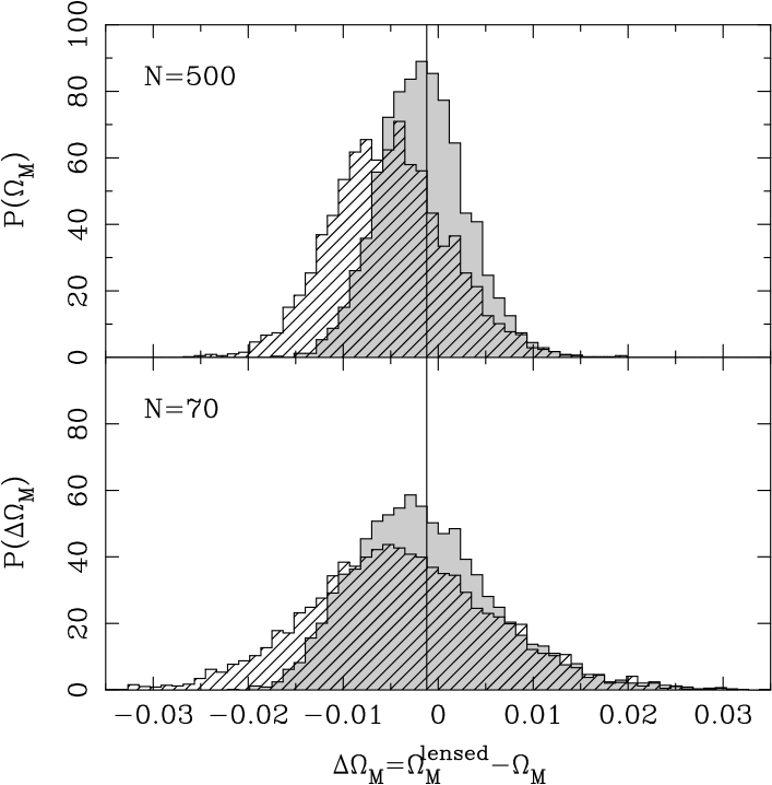
Figure 1: Shift in $\Omega_{\rm M}$ due to gravitational lensing. The grey shaded distributions show $\Delta\Omega_{\rm M}=\Omega_{\rm M}^{\rm lensed}-\Omega_{\rm M}$ for $\sim 5000$ simulated data sets consisting of 70 (bottom panel) and 500 (top panel) SNLS SNe Ia. The vertical solid line shows the shift ($\Delta\Omega_{\rm M}=-0.0012$) expected due to higher order moments of the magnification distribution. The hatched histograms show the shift which would be the result of removing bright $2.5\sigma$ outliers from the Hubble diagram.

Let us now consider the shift for case 2. Figure 2 shows the results of our simulations for SNLS. To each simulated data set, $\Omega_{\rm M}$ and $w$ were fitted simultaneously with and without lensing. The shaded histograms in the top and bottom panel in Fig. 2 show the probability distributions of $\Delta w$ for $N=500$ and $N=70$, respectively. Since the shift in $\Omega_{\rm M}$ is very small for case 2, we only consider $\Delta w$. Also for case 2 the expected bias, $\langle\Delta w\rangle$, is close to what we expect due to the higher order moments in the magnification factor distribution (outlined by the vertical lines in the figure).

The most likely shift for $N=70$ is $\Delta w\approx-0.005$, which is half the maximum shift ($\Delta w=-0.01$) estimated by Astier et al. (2006). The uncertainty in $w$ from gravitational lensing at the $1\sigma$ confidence level for the first year and final SNLS data together with BAO constraints is expected to be at the percent and sub-percent level, respectively. Most of this uncertainty, as already noted, should be included in the intrinsic scatter derived for the SNLS.

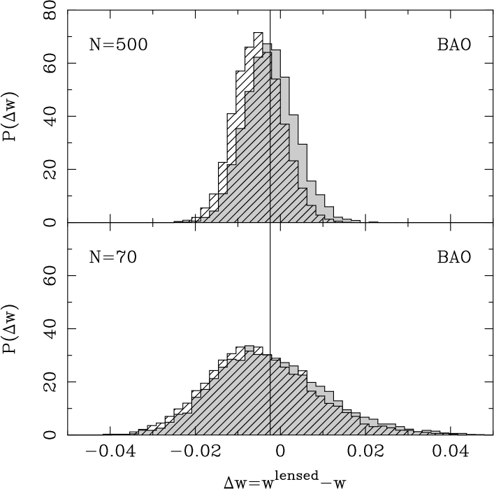
Figure 2: Shift in $w$ due to gravitational lensing. The grey shaded distributions show $\Delta w=w-w^{\rm lensed}$ for $\sim 5000$ simulated data sets consisting of 70 (bottom panel) and 500 (top panel) SNLS SNe Ia. The vertical solid line shows the shift ($\Delta w=-0.0024$) expected due to higher order moments of the magnification distribution. The hatched histograms show the shift which would be the result of removing bright $2.5\sigma$ outliers from the Hubble diagram. Constraints from BAO were used in the cosmology fits.

5.3 Removal of outliers

Since the magnification distribution is asymmetric, it is important to sample the high magnification tail. Highly magnified SNe Ia would be outliers in the Hubble diagram and might therefore be removed.

Sarkar et al. (2008) recently quantified the shift in the equation of state parameter which could be expected due to lensing for future large data sets ($\ga 2000$) of SNe Ia. They also investigated the effect of removing bright outliers. According to their simulations, the shift in $w$ increases from $\sim 0.5\%$ to $\sim 0.8\%$ when bright SNe Ia deviating by more than $2.5\sigma$ are removed.

We have performed a simple exercise to investigate the effects of removing highly magnified SNe Ia from the Hubble diagram. The hatched histograms in Figs. 1 and 2 show the effect of removing bright $2.5\sigma$ outliers. Approximately $1\%$ of the SNe Ia are removed by this cut. The results of the exercise are given in Table 1.

Let us first discuss the effect of removing bright outliers for case 1. If bright outliers are removed, the peak of the distribution of $\Delta\Omega_{\rm M}$ is shifted to a lower value. Moreover, the distribution broadens and become more gaussian. Since the high magnification SNe Ia have been removed, most SNe Ia appear to be dimmer and consequently the data favour a smaller value of $\Omega_{\rm M}$. The removal of the asymmetric high magnification tail also explains why the distribution of $\Delta\Omega_{\rm M}$ becomes more gaussian. The average shift in $\Omega_{\rm M}$ increases with approximately a factor $3$ when the outliers are removed.

The peak of the distributions shift towards lower values also for case 2. The shift in $w$ increases by a factor approximately $2$ when the bright outliers are removed. However, the width of the distributions hardly change at all.

5.4 Detecting a magnification correlation

Since amplified and de-amplified SNe Ia should be brighter and fainter than average, respectively, we expect a correlation between the residuals in the Hubble diagram and the estimated lensing magnifications, $\Delta_{\mu}$. Clearly, intrinsic brightness scatter among the SNe Ia as well as measurement errors add noise to the gravitational lensing signal. The ability to detect the correlation therefore depends on the quality and size of the data set.

Our simulations demonstrate that the quality of the SNLS data is sufficient for a detection of a correlation at high confidence. Figure 3 shows the probability of detecting the correlation at $1\sigma$ ($68.3\%$, solid curve), $2\sigma$ ($95.4\%$, dashed curve), and $3\sigma$ ($99.7\%$, dotted curve) confidence level as a function of the number of SNe Ia. For these simulations we have used the distributions of redshifts and errors from the first year of SNLS data (Astier et al. 2006). If the magnification factor could be estimated for $450$ SNe Ia, the probability to detect the correlation at the $3\sigma$ confidence level is $97.6\%$. A firm detection of the correlation between magnifications and SN Ia brightnesses is thus very likely to be found from the final SNLS data. If the magnification factor could be predicted exactly, the probability would instead be $99.9\%$. Even in this best case scenario uncertainties in the Hubble diagram residuals would affect our possibility to find the correlation.

Increasing the intrinsic brightness dispersion from $\sigma_{\rm int}=0.13$ mag to $\sigma_{\rm int}=0.15$ mag and $\sigma_{\rm int}=0.17$ mag would decrease the probability to make a $3\sigma$ detection of the lensing signal from $97.6\%$ to $96.1\%$ and $90.2\%$, respectively. The possibility to detect a lensing signal at high confidence level is thus not critically dependent on the intrinsic dispersion.

Our chances to make a high confidence level detection of the correlation using the final SNLS data looks promising even if our estimates of the lensing masses would be wrong. The probability to make a $3\sigma$ detection is $\ga 95\%$ even when the lensing masses are over-estimated or under-estimated by $\sim 50\%$. For the final SDSSIISN data set consisting of $\sim 300$ SNe Ia, on the other hand, we predict the probability of a $3\sigma$ detection to be only $4\%$.

Figure 3: Probability to detect a correlation between estimated magnification and SN Ia brightness at different confidence levels, $P(n\sigma)$, as a function of the number, $N$, of SNe Ia. The solid, dashed, and dotted curves shows the probability to detect a correlation at the $1\sigma$, $2\sigma$, and $3\sigma$ confidence level, respectively. The simulated data sets have the same distributions of redshifts and errors as the first year SNLS data.

5.5 Constraints on halo masses

The gravitational lensing signal provided by the correlation between magnifications and SN Ia brightnesses should also give some constraints on masses of the haloes of the lensing galaxies. We have performed simulations where the mass of each halo has been multiplied by a factor $F$. The increase or decrease in halo masses is compensated for by changes in the smoothness parameter to ensure that the total mass in the Universe sums up to the global value. To each simulated data set, a linear relation, $\Delta=A+B\Delta_{\mu}$, was fitted. Figure 4 shows how the slope, described by the parameter $B$, changes with the value of $F$. The dashed horizontal line corresponds to $B=1$, which is the value which would be recovered if the magnification factors were exactly known. If obvious outliers in the magnification-residual diagram are removed, the distribution of the $B$ parameter is gaussian. The inner and outer error bars in Fig. 4 correspond to $1\sigma$ and $2\sigma$ errors. The number of SNe Ia was $N=450$, however the standard deviation scales roughly as $1/\sqrt{N}$.

According to Fig. 4 the slope in the magnification-residual diagram varies with $F$, which should allow us to probe the normalisation of the halo masses. From the figure we conclude that the normalisation of the halo masses could probably be constrained with the final SNLS data set at the $1\sigma$ and $2\sigma$ confidence level with $\sim 30\%$ and $\sim 60\%$ accuracy, respectively.

Figure 4: Slope, $B$, in the magnification-residual diagram as a function of the factor $F$ which all halo masses have been multiplied by. The vertical dashed line shows the value expected for a correlation, i.e. $B=1$. The inner and outer errorbars correspond to $1\sigma$ and $2\sigma$ confidence level, respectively.

6 Conclusions

We have simulated the effect of gravitational lensing in two major ongoing supernova surveys. For the relatively nearby SDSSII supernova search, the effect of gravitational lensing will be small. For the more distant supernovae in the SNLS survey, we predict that the signal from gravitational lensing will be observed with high confidence. Our simulations indicate that a correlation between Hubble diagram residuals and magnification for individual supernovae will be present at high (at least $3\sigma$) significance level. This could be used both to somewhat reduce the scatter in the Hubble diagram, and to learn about the properties of the lensing material. A project to investigate this effect in the SNLS data is underway. We also note that the prospects of using weak lensing of supernovae to constrain the matter distribution in the Universe with future surveys such as SNAP look very promising. A satellite like SNAP would provide not only high redshift SNe Ia, but also deep observations in many filters which would allow reliable photometric redshifts of the galaxies to be obtained.