Instability of wormholes supported by a ghost scalar field. II. Nonlinear evolution
Abstract
We analyze the nonlinear evolution of spherically symmetric wormhole solutions coupled to a massless ghost scalar field using numerical methods. In a previous article we have shown that static wormholes with these properties are unstable with respect to linear perturbations. Here, we show that depending on the initial perturbation the wormholes either expand or decay to a Schwarzschild black hole. We estimate the time scale of the expanding solutions and the ones collapsing to a black hole and show that they are consistent in the regime of small perturbations with those predicted from perturbation theory. In the collapsing case, we also present a systematic study of the final black hole horizon and discuss the possibility for a luminous signal to travel from one universe to the other and back before the black hole forms. In the expanding case, the wormholes seem to undergo an exponential expansion, at least during the run time of our simulations.
pacs:
04.20.-q, 04.25.D-, 04.40.-bI Introduction
Motivated by spectacular predictions such as interstellar travel and time machines mMkT88 ; mMkTyU88 ; Visser-Book there has been a lot of interest in wormhole physics over the last years. Although wormhole geometries are speculative because they require exotic matter in order to represent consistent solutions of Einstein’s field equations, recent cosmological observations (see ghostcosmo1 for a review) may suggest the existence of phantom energy which could in principle be used to support a wormhole sS05 ; fL05 ; fL05b .
Assuming that stationary wormholes do exist within a particular matter model, a relevant question is whether or not they are stable with respect to perturbations. Motivated by this question, in a previous paper jGfGoS-inprep1 we performed a stability analysis of static, spherically symmetric wormhole solutions supported by a minimally coupled massless ghost scalar field. As we proved, such wormhole solutions are unstable with respect to linear, spherically symmetric perturbations of the metric and the scalar field. More specifically, we showed that each such solution possesses a unique unstable mode which grows exponentially in time, is everywhere regular and decays exponentially in the asymptotic region. The time scale associated to this mode is of the order of the areal radius of the wormhole throat divided by the speed of light.
The aim of this paper is twofold. First, we verify the wormhole instability predicted by the linear stability analysis carried out in our previous paper. For this, we first construct analytically initial data which describes a nonlinear perturbation of the data induced by the equilibrium configuration on a static slice. The time evolution of this data is obtained by numerically integrating the nonlinear field equations and we show that small initial perturbations do not decay to zero but grow in time and eventually kick the wormhole throat away from its equilibrium configuration. The growth of the departure of the areal radius of the throat from its equilibrium value as a function of proper time at the throat is computed for different parameters of the initial perturbation and shown to agree well with the time scale predicted by the perturbation calculation.
Our second goal is to determine the end state of the nonlinear evolution. We find that depending on the details of the initial perturbation the wormhole either starts expanding or collapsing. In the collapsing case, we observe the formation of an apparent horizon. By computing geometric quantities at the apparent horizon, we obtain a strong indication that the apparent horizon eventually settles down to the event horizon of a Schwarzschild black hole. By analyzing the convergence of light rays near the apparent horizon we obtain an estimate for the location of the event horizon and find that although asymptotically it seems to agree with the location of the apparent horizon it lies inside it at early times. Despite the rapid collapse, we find that it is possible for a photon to travel from one universe to the other and back without falling into the black hole. In the expanding case, we do not observe any apparent horizons and our simulations suggest that the wormhole expands forever. In particular, for wormholes which are reflection symmetric we find that the areal radius at the point of reflection symmetry grows exponentially as a function of proper time. Furthermore, we point out some problems with defining the wormhole throat in an invariant way. Specifically, we show that the definition of the throat as a minimum of the areal radius over each time-slice does not yield an invariant three surface, and we give an example showing that this three surface depends on the slicing condition.
Furthermore, we perform a careful study for the relation between the radius of the apparent horizon of the final black hole and the amplitude of the perturbation. By varying this amplitude, three regions are found: i) positive values of the amplitude result in the collapse to a black hole, ii) negative values of the amplitude lying sufficiently close to zero trigger the explosion of the solution, iii) a second threshold for the amplitude is found on the negative real axis below which the wormholes collapse to a black hole.
This paper is organized as follows. In section II we formulate the Cauchy problem for obtaining the nonlinear time evolution of spherically symmetric configurations, review the static wormhole solutions and describe our method for obtaining initial perturbations thereof. Our numerical implementation and the diagnostics we use in order to test our code and analyze the data obtained from the evolution are described in section III. In section IV we analyze the collapsing case and indicate that the final state is a Schwarzschild black hole. By analyzing the resulting spacetime diagram we also mention different scenarios for a light ray to travel from one universe to the other and back. The expanding case is analyzed in section V and the study for the relation between the final state and the amplitude of the perturbation is carried out in section VI. Finally, we summarize our findings and draw conclusions in section VII.
Some of the conclusions presented in this paper have been presented in Ref. hSsH02 for the wormholes with zero ADM masses based on a numerical method using null coordinates.
II The Cauchy problem for time-dependent solutions
In this section we formulate Einstein’s equations coupled to a massless ghost scalar field in a suitable form for the numerical integration of spherically symmetric wormhole solutions. We use geometrized units for which the speed of light and Newton’s constant are equal to one. We write the metric in the form
| (1) |
where the functions , and depend only on the time coordinate and the radial coordinate . Similarly, we assume that the scalar field only depends on and . The coordinate ranges over the whole real line, where the two regions and describe the two asymptotically flat ends. In particular, we require that the two-manifold is regular and asymptotically flat at , and that the areal radius is strictly positive and proportional to for large . For this reason, it is convenient to replace by where
| (2) |
and is a parameter. Next, we find it convenient to choose the following family of gauge conditions:
| (3) |
which relates the lapse to the functions and parametrizing the three-metric. Here, is a parameter that may take any real value in principle, but for our simulations we will consider the choices and . The metric now takes the form
| (4) |
II.1 Evolution and constraint equations
Einstein’s equations yield the Hamiltonian constraint , the momentum constraint and the evolution equations and , where here and refer, respectively, to the components of the Einstein and Ricci tensor, and and . These evolution equations, together with the wave equation for yield the following coupled system of nonlinear wave equations for the quantities , and :
| (5) | |||
| (6) | |||
| (7) |
which is subject to the constraints
| (8) | |||||
| (9) |
For we see that the principal part of the evolution equations is given by the flat wave operator . Therefore, the characteristic lines coincide with the radial null rays which for are given by the straight lines Therefore, a property of the gauge condition (3) with is that it cannot lead to shock formations due to the crossing of characteristics. We found this gauge to be convenient for studying expanding wormholes. For the collapsing case, on the other hand, we found the gauge (3) with more useful since it seems to be avoiding the singularity after the black hole forms.
II.2 Propagation of the constraints
It can be shown that the Bianchi identities and the evolution equations (5,6,7) imply that the constraint variables and satisfy a linear evolution system of the form
| (10) | |||||
| (11) |
where are lower order terms which depend only on and but not their derivatives. For a solution on the unbounded domain with initial data satisfying it follows that the constraints are automatically satisfied everywhere and for each . Therefore, it is sufficient to solve the constraints initially. If artificial time-like boundaries are imposed, this statement is still true provided suitable boundary conditions are specified. For example, imposing the momentum constraint at the boundary ensures that the constraints remain satisfied if so initially.
II.3 Boundary conditions
Since we have three wave equations, at the artificial boundaries we apply outgoing wave boundary conditions for the three fields , and . We assume that these fields behave like spherical waves far away from the origin, i.e. if :
| (12) |
where is the speed of propagation. In order to apply the boundary conditions, we use the following equation,
| (13) |
We use a similar procedure when . It is clear that such conditions do not preserve the constraints and consequently, the solution will be contaminated with a constraint-violating pulse traveling inwards in the numerical domain. In order to avoid the contamination of the analyzed data, we push the boundaries far from the throat such that the region where we extract physics is causally disconnected from the boundaries.
II.4 Static wormhole solutions
In the static case, all wormhole solutions can be found analytically hE73 ; kB73 ; cA02 and are given by the following expressions
| (14) | |||||
| (15) | |||||
| (16) |
where the parameters and are subject to the condition . The wormhole throat is located at and has areal radius . The ADM masses at the two asymptotically flat ends are and , respectively (see Ref. jGfGoS-inprep1 for a derivation and details). In particular, yields wormhole solutions with zero ADM mass at both ends while in all other cases the ADM masses at the two ends have opposite signs.
II.5 Initial data describing a perturbed wormhole
In order to study the nonlinear stability of the static solutions described by equations (14,15,16) we construct initial data corresponding to an initial perturbation of a static solution. For simplicity, we assume that the initial slice is time-symmetric in which case the momentum constraint is automatically satisfied. Therefore, we only need to solve the Hamiltonian constraint which, for simplifies to
| (17) |
Since the unperturbed wormhole solution is known in analytic form a simple way of obtaining initial data representing a perturbation thereof is to perturb the metric quantities and by hand in such a way that the left-hand side of equation (17) is nonnegative and to solve equation (17) for . Since the left-hand side of Equation (17) is everywhere positive for the analytic solution, it remains positive at least for small enough perturbations. Moreover, it is clear that any time-symmetric and spherically symmetric initial data can be obtained by this method. Next, we notice that it is sufficient to consider the case where the metric component is unperturbed. Indeed, a perturbation of may be absorbed by a redefinition of the coordinate which, at the physical level, does not change the initial data and its Cauchy development. Therefore, it is sufficient to perturb the quantity which is related to the areal radius. For this work, we choose to perturb it with a Gaussian pulse. More precisely, we choose
| (18) | |||||
| (19) |
where is the amplitude, the center and is related to the width at half maximum of the pulse through . As will be shown later, different values of and produce two different scenarios: the collapse of the wormhole to a black hole or a rapid expansion. Notice that because of the exponential decay of the perturbation as , the ADM masses of the perturbed solution is equal to the ADM masses of the unperturbed, static solution.
III Implementation and diagnostics
In this section we describe our numerical method and different tools used to analyze the data obtained from the simulations. The numerical method is based on a second order centered finite differences approximation of the evolution equations (5-7) and the constraint equations (8,9). We only perform the evolution on a finite domain with artificial boundaries at a finite value of where we implement the radiative-type boundary condition (13) with an accuracy of second order for the evolution variables , and . A method of lines using the third order Runge-Kutta integrator is adopted. Throughout the evolution, we monitor the constraint variables and and check that they converge to zero as resolution is increased.
From now on we rescale the coordinate in such a way that .
III.1 Unperturbed wormhole
As a test, using the implementation aforementioned we perform a series of simulations for the unperturbed, static wormholes. We start a simulation with the massless case , for which it is expected that the fields remain time-independent. However, discretization errors are enough to trigger a non-trivial time dependence of these functions. We have verified that when increasing the resolution, the numerical error remains small for a larger period of time and the numerical solution converges to the exact, static solution with second order. In figure 1 we show the convergence of the constraint variable for a wormhole using the gauge parameter .
III.2 Extremal and marginally trapped surfaces
Let us consider a hypersurface . There are two different types of interesting two-surfaces in this hypersurface: The first are extremal surfaces which consist of two-surfaces with a local extrema of their area. If denotes the unit normal to this surface, this means that the divergence vanishes, where refers to the covariant derivative associated to the induced three-metric on . The second type of two-surfaces of interest are marginally trapped surfaces. Denoting by and the future-pointing outward and inward null-vectors orthogonal to this two-surface, a marginally trapped surface is defined by the requirement that the expansion along is strictly negative while the expansion along vanishes. In terms of the induced metric on the two-surface, this means that
Notice that a rescaling of or by a positive function does not affect this definition. On the other hand, for wormhole topologies the notions “outward” and “inward” are observer-dependent: they depend on which asymptotic end these vectors are viewed from.
With respect to slices of the spherically symmetric metric (1) we have , , (with respect to the asymptotic end ), and
| (20) |
Therefore, an extremal surface is a sphere for which , and a marginally trapped surface a sphere for which and . In particular, according to our definition, an extremal surface cannot be a marginally trapped surface. Finally, we define a throat to be an extremal surface which (out of the many extremal surfaces that might exist) is one with least area. In a similar way, an apparent horizon is an outermost marginally trapped surface. Notice that these concepts are not defined in a geometrically invariant way. For example, it is known rWvI91 that the Schwarzschild spacetime possesses Cauchy surfaces which do not contain any trapped surfaces and nevertheless come arbitrarily close to the singularity. Similarly, we will provide a numerical example below that shows that the three-surface obtained by piling up the throats in each time slice is not invariant but depends on the time foliation.
III.3 Geometric quantities
Throughout evolution, we monitor the values of the following geometric quantities:
| (21) | |||||
| (22) | |||||
| (23) |
where quantities with a tilde refer to the two-metric . As mentioned above, is the areal radius of the sphere at constant and . is the Misner-Sharp mass function cMdS64 and is the norm of the gradient of the scalar field. In particular, the knowledge of these functions allows the computation of the following curvature scalars: The Ricci scalar associated to the two-metric , the Kretschmann scalar associated to the full metric , and the square of the Ricci tensor, . Using Einstein’s field equations one obtains the following expressions,
| (24) | |||||
| (25) | |||||
| (26) |
III.4 The construction of conformal coordinates
The gauge choice (3) with has the property of yielding conformally flat coordinates for the two-metric . In these coordinates, the null rays are simply given by the straight lines
On the other hand, in many simulations, the choice seems to work better than the choice . In order to compare the coordinates , say, constructed with the gauge choice to the conformally flat coordinates obtained with one can proceed as follows. Suppose we are given to us a two-metric with signature . We are interested in finding local coordinates such that
| (27) |
with a conformal factor . We first note that if denotes the volume element associated to , the coordinates and must satisfy
| (28) |
since by equation (27) and are orthogonal to each other and their norms are equal in magnitude. It follows from equation (28) that and must also satisfy the wave equation
| (29) |
Therefore, in order to construct the coordinates , we have to solve equations (29) subject to the constraint (28). The resulting functions indeed satisfy (27) since
The conformal factor is then obtained from . Notice that equation (29) implies that both and are conserved, i.e. . Therefore, it is sufficient to solve the constraint on a Cauchy slice.
For example, suppose that as is the case for our simulations with . Then, equations (29) yield
and the initial data for the functions and satisfies
The last two equations follow from equation (28) where we have chosen the sign such that and point in the same direction. The so obtained functions and can be used, for instance, to plot a surface in the diagram. They may also be useful to find the null rays which are given by the lines with constant or .
IV Collapse to a black hole
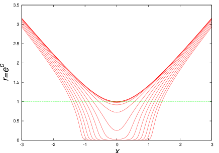
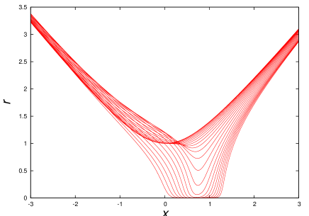
For simplicity, we start with the evolution of a perturbed, massless wormhole with the perturbation consisting of a Gaussian pulse as in (19) with so that the perturbation is centered at the throat. We start with positive values of the amplitude and find that such perturbations induce a collapse of the throat. The typical behaviour of such a collapsing wormhole is presented in figures 2 to 9.
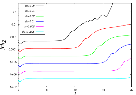
In figure 2 we show the convergence of the Hamiltonian constraint as a function of coordinate time and the evolution of the areal radius which exhibits the collapse of the wormhole throat.
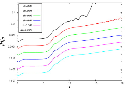
IV.1 Time scale of the collapse
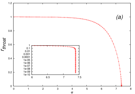
In order to check the consistency of our numerical calculations with the time scale associated to the unstable mode found in our linear stability analysis, we perform a systematic study of the speed of the collapse of the throat. For simplicity, we only consider massless wormholes with a centered perturbation. Our procedure for quantifying the speed of the collapse is the following:
-
i)
Compute at each time the throat’s location by finding the minimum of the areal radius. For the reflection symmetric case, this minimum is located at .
-
ii)
Compute the proper time integrating the lapse function at the throat.
-
iii)
Plot the throat’s areal radius as a function of proper time.
-
iv)
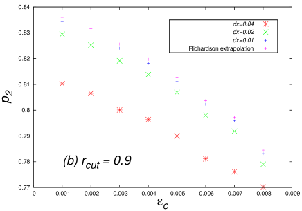
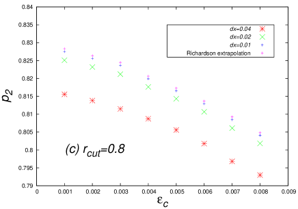
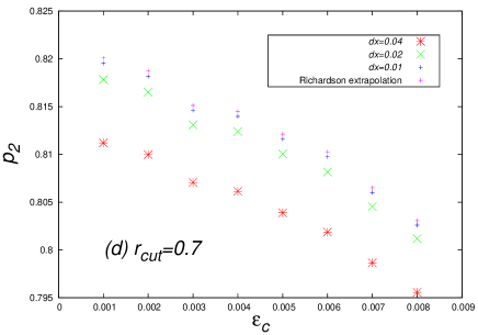
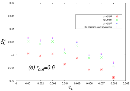
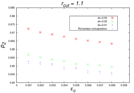
Fit the throat’s areal radius as a function of proper time to the function , from the initial radius of the throat until a chosen minimum value of , called . We interpret the parameter as the time scale of the solution. The reason to cut off the values of is that we want to compare with the results from perturbation theory which are expected to be valid as long as the departure from the equilibrium configuration is small.
-
v)
Repeat the above analysis for fixed initial parameters and and several values of the amplitude .
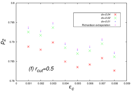
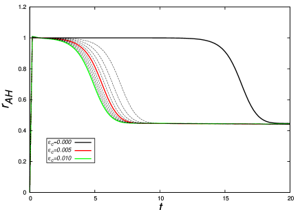
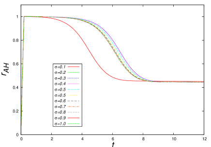
In figure 3 we show the results for the time scale and its dependency on the cut-off value , the initial parameter and the resolution used for the numerical evolutions. Two main features are: 1) The time scale for small values of and approach the one calculated from linear perturbation theory jGfGoS-inprep1 , 2) for large values of and small values of , the time scale is always smaller than the result of perturbation theory, indicating that nonlinear terms tend to accelerate the collapse.
IV.2 Formation of an apparent horizon
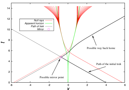
During the collapse, we observe the formation of an apparent horizon. This is shown in the left panel of figure 4, where we also show a bundle of outgoing null rays whose intersection points with the initial slice are fine-tuned in such a way that these rays lie as close as possible to the apparent horizon for late times. As the plot suggests, this bundle of light rays separates photons that might escape to future null infinity from photons that are trapped inside a region of small . Therefore, we expect this bundle to represent a good approximation for the event horizon of a black hole. As a consequence, our simulations give a strong indication for the collapse of the wormhole into a black hole.
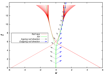
The bold black line in the left panel of figure 4 indicates a possible trajectory of a photon traveling from one universe to the other and back, allowing it to reach the asymptotic region of the home universe without getting trapped by the black hole. In the right panel the future null directions at the apparent horizon location are presented, showing that the latter is a time-like surface.
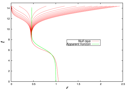
Somehow unusual features of the collapse are that the apparent horizon is not contained in the black hole region and that the areal radius of both the apparent and event horizons decreases in time. This is illustrated in figure 5, where we plot the trajectory of the apparent horizon and the bundle of outgoing null rays in the diagram. Notice that for a spacetime satisfying the null energy condition and cosmic censorship, propositions 9.2.1 in HawkingEllis-Book and 12.2.3 in Wald-Book show that an apparent horizon is contained in the black hole region. Under the same assumptions theorem 12.2.6 in Wald-Book and sH71 ; pCeDgGrH01 establish that the area of the event horizon cannot decrease in time. In the present case, these results do not apply since the null energy condition is not satisfied. The decrease of the area of the horizons could be related to the absorption of the ghost scalar field by the black hole.
IV.3 The final state
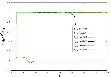
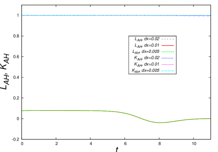
In order to analyze the final state of the collapsing wormholes we compute the scalars and from equations (22,23) at the apparent horizon location. At the event horizon of a Schwarzschild black hole these scalars are zero and one, respectively. As shown in figure 6, these quantities do indeed converge to the corresponding Schwarzschild values for large times and high spatial resolutions, indicating that the final state is a Schwarzschild black hole, at least in the vicinity of the apparent horizon.
We try different initial parameters and perform runs with centered and off-centered perturbations, and in all cases where the wormhole starts collapsing the result is the same: an apparent horizon forms, and it seems to settle down to the event horizon of a Schwarzschild black hole. We also investigate the mass of the final black hole as a function of the parameters of the perturbation. In figure 7 we present the evolution of the apparent horizon radius as a function of coordinate time for small, positive values for the amplitude and different values for the width . For such values it seems that the final black hole mass is universal and given by . The dependency of the black hole’s final areal radius for a wider range of initial parameters will be analyzed in section VI.
IV.4 The distribution of the scalar field
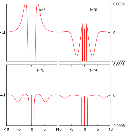
In order to investigate the time evolution of the distribution of the scalar field, we show in figure 8 snapshots at different times of along the spatial domain for the collapse of a zero mass configuration. A pulse of scalar field departs from the location of the apparent horizon region and propagates outwards with negative values. Since we know that the ADM mass of the spacetime is zero and that the mass of the apparent horizon is positive, we expect these pulses of scalar field to radiate negative energy.
Finally, we also analyzed the collapse of massive wormholes which are characterized by a positive value of the parameter . The results are qualitatively similar to those found for the zero mass case. For completeness, we show the behaviour of the areal radius for a collapsing case and the scalars calculated at the apparent horizon in figure 9.
V The expanding case
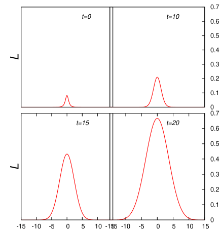
Perturbations that do not result in a collapse to a black hole induce a rapid growth of the wormhole throat. In order to analyze this case, we performed a series of simulations for the perturbed wormhole solutions starting with the massless case . In figure 10 we consider the evolution of a reflection symmetric perturbation and show the areal radius of the spheres at the points of reflection symmetry as a function of proper time. The exponential growth of this function indicates a rapid growth of the wormhole.
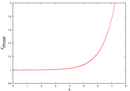
V.1 Time scale of the expansion
Also shown in figure 10 is the time scale associated to the exponential growth for different resolutions and different values of the initial amplitude of the perturbation. The function used to fit the radius of the throat in this case is . In the limit the time scale is estimated to be which is in good agreement with the prediction from perturbation theory, see Table I in Ref. jGfGoS-inprep1 .
V.2 Slice-dependence of the throat
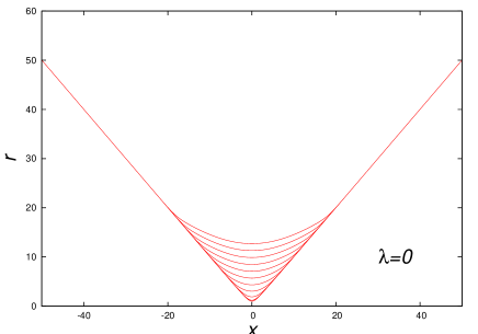
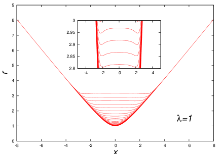
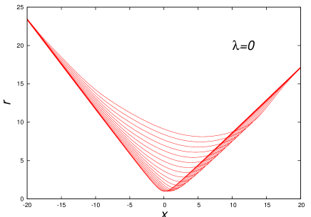
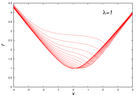
Next, we performed runs with the two gauge values and with perturbations centered at the throat. While we did not find the formation of any apparent horizons in any of these two gauges, there is an interesting difference in the behaviour of the areal radius as a function of the coordinate. This is shown in figure 11. For this function always has its minimum at , and one is tempted to define the throat’s location to be at . However, looking at the results for , one finds that although initially the minimum of as a function of lies at , at late times the function possesses a maximum at and two minima, one at a negative value of and the other at a positive value of . Therefore, from the results with , one is led to the conclusion that two throats develop.
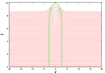
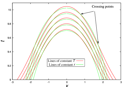
It turns out that this apparent paradox is an effect of the different slicing conditions resulting from the gauge condition (3) with and , respectively. In order to explain this, denote by the conformal coordinates corresponding to the evolution with , and let denote the coordinates obtained in the evolution with . The relation between these two coordinate systems can be obtained from the method described in section III.4. In figure 12 we show a spacetime diagram based on the conformal coordinates where we plot the surfaces of constant areal radius and the space-like slices of constant . As can be seen, at late enough times, the surfaces of constant may cross the lines of constant areal radius four times. Therefore, as one moves along a slice from one asymptotic end towards the other, the areal radius decreases until a minimum is reached, then the areal radius increases again until a local maximum is reached at ; then decreases again until a local minimum is reached, and finally the areal radius increases again. Therefore, the two-throat image is a pure gauge effect, and the definition of the throat’s location as a local minimum of the areal radius over a given time slice is not defined in a geometrical invariant way, but strongly depends on the time foliation.
V.3 The distribution of the scalar field
In order to investigate the time evolution of the distribution of the scalar field for the expanding case we show in figure 13 snapshots at different times of the scalar along the spatial domain for the expansion of a zero mass wormhole. As can be seen from this plot, the amplitude of this quantity increases in time while its shape remains essentially the same. Therefore, in contrast to the collapsing case, the scalar field does not seem to dissipate away but actually gains in strength near the point of reflection symmetry .
Finally, we also perform an evolution for a massive wormhole with . This is shown in figure 14.
VI Dependency of the final state on the initial perturbation
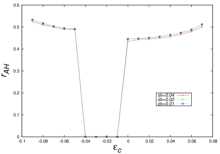
We want to analyze the dependency of the final state of the system on the initial perturbation. As we mentioned before, the two possible final states of the evolution are the collapse into a black hole or the expansion of the throat. In the former case, we can measure the radius of the apparent horizon of the final black hole. In the latter, there is no formation of black holes. We perform a systematic analysis on the dependency of the apparent horizon’s areal radius as a function of the initial perturbation. As before, we perturb the function with a Gaussian pulse centered at with fixed width , varying the amplitude from to in intervals of . When the values of the amplitude are positive the system collapses into a black hole. We found that the radius of the black hole decreases from for to for . Once the values of the amplitude become negative the behaviour of the evolution changes. In the interval the wormhole expands instead of collapsing and no apparent horizon is found. It is tempting to stop here and assume that this behaviour will continue. Nevertheless, if we keep decreasing the value of the amplitude we find that for values in the interval the system collapses again into a black hole. In this range, the radius of the black hole increases from to . These results are presented in figure 15 for three different resolutions in order to emphasize the convergence of the apparent horizon’s areal radius.
VII Conclusions
Based on numerical methods, we analyzed in this work the nonlinear stability of static, spherically symmetric general relativistic wormhole solutions sourced by a massless ghost scalar field. This complements the linear stability analysis performed in jGfGoS-inprep1 where we proved that all such solutions are unstable with respect to linear fluctuations. In particular, our numerical simulations confirm the instability predicted by linear theory and show that static, spherically symmetric wormholes sourced by a massless ghost scalar field are also unstable with respect to nonlinear fluctuations. Furthermore, we have checked that the time scale associated to the instability agrees with the one computed from perturbation theory, at least when computed over times for which the departure from the equilibrium configuration is small.
Our numerical simulations also reveal that depending on the initial perturbation, the wormholes either collapse to a Schwarzschild black hole or undergo a rapid expansion. This confirms the results in hSsH02 in the zero mass case and shows that a similar result holds for massive wormholes. In the collapsing case, we reach this conclusion by first observing the formation of an apparent horizon whose areal radius converges to a fixed positive value at late times. By computing geometrical quantities at the apparent horizon and analyzing the behaviour of null geodesics in the vicinity of the apparent horizon at late times we are led to the conclusion that the final state of the collapse is a Schwarzschild black hole. Further clues in support of this scenario are provided by the observation that the scalar field disperses.
In the expanding case, the wormhole starts growing rapidly. For reflection symmetric wormholes we find that the areal radius of the spheres at the points of reflection symmetry grow exponentially with respect to proper time. On the other hand, we have also found that the definition of the throat as the three-surface obtained by determining the global minimum of the areal radius in each time slice is problematic in the sense that it may depend on the time foliation.
We have also performed a systematic study of the dependency of the final state on the initial parameters of the perturbation. Using only reflection symmetry initial data with a Gaussian perturbation profile we investigated the possible universality of the final black hole’s mass. We found that for small, positive amplitudes of the initial perturbation the final mass does not vary much with respect to the initial width of the perturbation. For initial amplitudes which are negative and small in magnitude, on the other hand, the wormholes expand, the limiting case of zero amplitudes corresponding to a threshold in parameter space separating collapsing wormholes from expanding ones. By exploring a wide region of negative values for the initial amplitude we also found a second threshold below which the wormholes collapse again into a black hole.
Since a tiny perturbation may cause the wormhole to collapse into a black hole, it is unlikely that the wormholes we have analyzed in this article are useful for interstellar travel or building time machines. Furthermore, the time scale associated to the collapse is of the order of the throat’s areal radius divided by the speed of light, which is of the order of a few microseconds for a throat with areal radius of one kilometer. We have analyzed the possible scenarios in which a test particle may use the wormhole to tunnel from one universe to the other and back before the black hole forms. As a consequence of the instability, an observer moving on the path of such a test particle cannot explore an arbitrarily large region of the other universe if he wants to travel back home.
Acknowledgements.
We thank Ulises Nucamendi and Thomas Zannias for many stimulating discussions. This work was supported in part by grants CIC 4.9, 4.19 and 4.23 to Universidad Michoacana, PROMEP UMICH-PTC-121, UMICH-PTC-195, UMICH-PTC-210 and UMICH-CA-22 from SEP Mexico and CONACyT grant numbers 61173, 79601 and 79995.References
- [1] M.S. Morris and K.S. Thorne. Wormholes in spacetime and their use for interstellar travel: A tool for teaching general relativity. Am. J. Phys., 56:395–412, 1988.
- [2] M.S. Morris, K.S. Thorne, and U. Yurtsever. Wormholes, time machines, and the weak energy condition. Phys. Rev. Lett., 61:1446–1449, 1988.
- [3] M. Visser. Lorentzian wormholes. From Einstein to Hawking. American Institute of Physics, Woodbury, New York, 1995.
- [4] E. J. Copeland, M. Sami, and S. Tsujikawa. Dynamics of dark energy. Int. J. Mod. Phys. D, 15:1753–1936, 2006.
- [5] S.V. Sushkov. Wormholes supported by a phantom energy. Phys. Rev. D, 71:043520, 2005.
- [6] F.S.N. Lobo. Phantom energy traversable wormholes. Phys. Rev. D, 71:084011, 2005.
- [7] F.S.N. Lobo. Stability of phantom wormholes. Phys. Rev. D, 71:124022, 2005.
- [8] J. A. González, F. S. Guzmán, and O. Sarbach. Instability of wormholes supported by a ghost scalar field. I. Linear stability analysis. http://arxiv.org/abs/0806.0608, to appear in Class. Quantum Grav.
- [9] Hisa aki Shinkai and Sean A. Hayward. Fate of the first traversible wormhole: Black hole collapse or inflationary expansion. Phys. Rev. D, 66:044005, 2002.
- [10] H.G. Ellis. Ether flow through a drainhole: A particle model in general relativity. J. Math. Phys., 14:104–118, 1973.
- [11] K.A. Bronnikov. Scalar-tensor theory and scalar charge. Acta Phys. Polonica B, 4:251–266, 1973.
- [12] C. Armendáriz-Picón. On a class of stable, traversable Lorentzian wormholes in classical general relativity. Phys. Rev. D, 65:104010, 2002.
- [13] R.M. Wald and V. Iyer. Trapped sufaces in the Schwarzschild geometry and cosmic censorship. Phys. Rev. D, 44:R3719–R3722, 1991.
- [14] C.W. Misner and D.H. Sharp. Relativistic equations for adiabatic, spherically symmetric gravitational collapse. Phys. Rev., 136:B571–B576, 1964.
- [15] S.W. Hawking and G.F.R. Ellis. The Large Scale Structure of Space Time. Cambridge University Press, Cambridge, 1973.
- [16] R.M. Wald. General Relativity. The University of Chicago Press, Chicago, London, 1984.
- [17] S.W. Hawking. Gravitational radiation from colliding black holes. Phys. Rev. Lett., 26:1344–1346, 1971.
- [18] P. T. Chrusciel, E. Delay, G. J. Galloway, and R. Howard. Regularity of horizons and the area theorem. Annales Henri Poincar\a’e, 2:109–178, 2001.