Application of B-splines to determining eigen-spectrum of Feshbach molecules

Abstract

The B-spline basis set method is applied to determining the rovibrational eigen-spectrum of diatomic molecules. A particular attention is paid to a challenging numerical task of an accurate and efficient description of the vibrational levels near the dissociation limit (halo-state and Feshbach molecules). Advantages of using B-splines are highlighted by comparing the performance of the method with that of the commonly-used discrete variable representation (DVR) approach. Several model cases, including the Morse potential and realistic potentials with $1/R^{3}$ and $1/R^{6}$ long-range dependence of the internuclear separation are studied. We find that the B-spline method is superior to the DVR approach and it is robust enough to properly describe the Feshbach molecules. The developed numerical method is applied to studying the universal relation of the energy of the last bound state to the scattering length. We numerically illustrate the validity of the quantum-defect-theoretic formulation of such a relation for a $1/R^{6}$ potential.

I Introduction

Finite basis sets technique is an important numerical tool in solving quantum mechanical problems, e.g., in quantum chemistry DavFel86 . One of the popular recent developments is the use of B-splines in such calculations. In atomic physics, the applications of B-splines were stimulated by Walter R. Johnson’s work JohBluSap88 and here, in this special issue dedicated to celebrating his contributions to atomic physics, we are delighted to present yet another robust application of B-splines.

The reason to the popularity of the B-splines in practical applications is due to the fact that they form a sufficiently complete basis set with a reasonably small number of basis functions. Numerical accuracy of the calculations approaches that of the traditional finite-difference methods, such as the Numerov method BacCorDec01 , with the advantage of a global non-iterative determination of eigenergies and eigenstates.

Here we apply the B-spline method to study rovibrational eigen-spectrum of diatomic molecules and compare the performance of the method with that of the discrete variable representation (DVR) approach. Previously, the B-spline method was successfully applied to finding vibrational spectrum of the Morse potential in Refs. BacCorDec01 ; Sho73 . Here we focus on the more challenging problem of describing vibrational states near the dissociation limit of realistic long-range potentials. One difficulty lies in the variation of the local de Broglie wavelength by several orders of magnitude from the short range to the long range region. Several authors kokoouline1999 ; WilDulMas04 have discussed how the efficiency of the DVR methods could be improved via the implementation of a mapping procedure, where the grid step is adapted to the variation of the de Broglie wavelength. In the present paper we compare the mapped sine grid method of Ref. WilDulMas04 to B-splines calculations also using a mapping procedure. Molecular bound states near dissociation limit play an important role in the formation of ultracold molecules masnou2001 ; doyle2004 and in the determination of scattering properties in the low-energy regime, in particular scattering length crubellier99 or more generally the threshold energy-dependence of the phaseshifts. The vibrational wavefunctions then extend to distances much larger than the typical length of the chemical bond. Recently several experimental groups succeeded in making loosely-bound ultracold molecules by sweeping B-fields through the magnetically-induced Feshbach resonances (see review KohGorJul06 ). Such Feshbach molecules may be considered as halo-state systems, since the vibrational wavefunctions extend well into the classically-forbidden region. While the halo-state systems, due to their universal behavior for a wide range of quantum-mechanical systems, deserve a special attention on their own right JenRiiFed04 , there are emerging applications based on the Feshbach molecules: for example, several schemes of transferring Feshbach molecules to lower vibrational levels and down to $v=0$ Koch2004 ; PerShaSto07 have been proposed. In the prerequisite numerical time–dependent studies, an expansion over a suitably-chosen quasi-spectrum is required, and the initial state near dissociation limit has to be well represented by this quasi–spectrum. The challenge there is the accurate representation of the evanescent part of the wavefunction in the non classical region. B-splines, with their superior numerical performance, demonstrated here, may prove useful in such theoretical studies. We shall therefore evaluate this performance by comparing to analytical results when available (bound levels of the Morse potential) or to well–established numerical methods.

Motivated by the spectacular developments in low-energy collision physics of ultracold atoms, the universal laws governing near-threshold physics have generated a considerable interest over the last decade. In particular, here, with the developed numerical method, we investigate a relation of the energy of the last bound state to the scattering length. For potentials without a long range tail, such a relation is a well-known prediction of the effective-range theory (see e.g., LanLif97 ). For the van der Waals potentials, the effective range theory has to be improved to account for their asymptotic behavior and Gao Gao04a has recently derived the proper law relating these two quantities in the framework of the quantum defect theory (QDT). Here, using the developed B-spline code, we verify numerically the validity of this new formulation. We find that compared to the effective-range result, the QDT expression remains accurate over a much wider range of parameters than expected.

The paper is organized as follows. First, in Section II, we set-up the numerical method using the Galerkin technique and expansion of the molecular wavefunctions over the B-spline basis. We also describe an efficient molecular grid used in the calculations and recapitulate main features of the DVR method. In Section III, we apply the method to finding ro-vibrational spectra of various potentials and compare the results with those from the DVR method. We start with the Morse potential, where analytical results are available, and proceed to realistic potentials, varying with the internuclear separations, $R$, as $1/R^{3}$ and $1/R^{6}$ at large $R$. With the developed method, in Section IV, we analyze the relation between the scattering length and the position of the last bound state and compare our numerical results with the predictions of the QDT and the effective-range theories. Finally, the conclusions are drawn in Section V.

II Problem setup

We are interested in solving the radial time-independent Schrödinger equation for vibrational motion of nuclei of a diatomic molecule

$$-\frac{1}{2\mu}u^{\prime\prime}_{J}\left(R\right)+\left(V\left(R\right)+\frac{J\left(J+1\right)}{2\mu R^{2}}\right)u_{J}\left(R\right)=$$ (1)

$$E\leavevmode\nobreak\ u_{J}\left(R\right)\,,$$

where $\mu$ is the reduced molecular mass, $J$ is the rotational quantum number and $V\left(R\right)$ is the electronic Born-Oppenheimer potential. Unless specified otherwise, atomic units, $\hbar=\left|e\right|=m_{e}\equiv 1$, are used throughout.

II.1 B-spline approach

General mathematical introduction to B-splines and a collection of codes to manipulate these basis functions may be found in Ref. deB01 . Here we briefly recapitulate properties of the B-splines relevant to our discussion. We deal with a set of $n$ functions defined on a support grid $\{t_{i}\}$. A B-spline, $B_{i}^{\left(k\right)}\left(R\right),$ number $i$ of order $k$ is a piecewise polynomial of degree $k-1$ inside an interval of the support grid $t_{i}\leq R<t_{i+k}$. It vanishes outside this support interval. The B-splines are positive functions on their support interval. In applications, the common choice (also used here) is to make the end-points of the support grid $k$-fold degenerate,

$$t_{1} = t_{2}=\cdots=t_{k}=R_{\min},$$

$$t_{n+1} = \cdots=t_{n+k}=R_{\max},$$

where $n$ is the total number of B-splines in the set. With such a choice of the grid, the first B-spline, $B_{i=1}^{\left(k\right)}\left(R\right)$ is the only spline which does not vanish at $R_{\min}$. Similarly, the only non-vanishing B-spline at the end-point $R_{\max}$ is the last B-spline, $B_{i=n}^{\left(k\right)}\left(R\right)$. Notice that the spline support grid ${t_{i}}$ directly maps on the radial grid, except the multiply defined end-points that map onto the first and last points of the radial grid.

Below, we employ the Galerkin method to obtain a quasi-spectrum of the radial Schrödinger equation, see, e.g., Joh07book . Central to this approach is an observation that the differential equation (1) may be derived by seeking an extremum of the action integral,

$$S = \int_{R_{\mathrm{min}}}^{R_{\mathrm{max}}}\left\{\frac{1}{2\mu}\left(\frac{du_{J}\left(R\right)}{dR}\right)^{2}+\right.$$

$$\left.\left(V\left(R\right)+\frac{J\left(J+1\right)}{2\mu R^{2}}\right)u_{J}^{2}\left(R\right)\right\}dR$$

$$-E\int_{R_{\mathrm{min}}}^{R_{\mathrm{max}}}u_{J}^{2}\left(R\right)dR.$$

Further, we expand the ro-vibrational wavefunctions in terms of the B-spline set,

$$u_{J}\left(R\right)=\sum_{i=2}^{n-1}c_{i}B_{i}^{\left(k\right)}\left(R\right).$$ (2)

Notice that we discard the first and the last B-spline of the set to enforce the boundary conditions $u_{J}\left(R_{\mathrm{min}}\right)=0$ and $u_{J}\left(R_{\mathrm{max}}\right)=0$. The remaining splines vanish identically at the end-points of the grid.

We substitute the expansion (2) in the action integral and seek its extremum with respect to the expansion coefficients. As a result, we arrive at the generalized eigen-value equation for the vector of the coefficients $\mathbf{c}=(c_{2},c_{3},...c_{n-1})$:

$$\mathbf{Ac}=E\leavevmode\nobreak\ \mathbf{B\leavevmode\nobreak\ c}\,,$$ (3)

with matrices

$$A_{ij} = \int_{R_{\mathrm{min}}}^{R_{\mathrm{max}}}\left\{\frac{1}{\mu}\frac{dB_{i}}{dR}\frac{dB_{j}}{dR}+\right.$$ (4)

$$\left.2B_{i}\left(V\left(R\right)+\frac{J\left(J+1\right)}{2R^{2}}\right)B_{j}\right\}dR,$$

$$B_{ij} = \int_{R_{\mathrm{min}}}^{R_{\mathrm{max}}}B_{i}B_{j}\leavevmode\nobreak\ dR.$$

The resulting eigenfunctions are orthonormal and form a numerically complete basis set in the space of piece-wise polynomials of order $k-1$. The choice of the number of basis functions is determined by the nodal structure of the wavefunctions that we wish to represent.

II.2 Mapped grid method

Choosing numerical grid for solving the radial Schrödinger equation for loosely bound molecules requires special consideration. Realistic potentials support a large number of bound states. Near the dissociation limit the corresponding wavefunctions have a large number of nodes. Moreover,the distance between two nodes, and hence the local De Broglie wavelength, grows larger as we approach the outer turning point of the potential. A large fraction of the wavefunction (especially for halo-state molecules) may reside in the classically-forbidden region. Because of this behavior of the vibrational states, here we depart from the usual choice of the radial grid of a constant step as in Refs. BacCorDec01 ; Sho73 . Instead, we employ a more efficient grid as prescribed by the “mapped grid” method of Ref. kokoouline1999 ; WilDulMas04 , first implemented in the framework of the DVR method described below.

In the “mapped grid” method the radial grid is based on the adaptive coordinate defined as

$$x\left(R\right)=\beta^{-1}\frac{\sqrt{2\mu}}{p_{\max}}\int_{R_{\mathrm{min}}}^{R}dR^{\prime}\sqrt{E_{\max}-V_{\mathrm{env}}\left(R^{\prime}\right)},$$

where $V_{\mathrm{env}}\left(R\right)$ is the enveloping potential (it is chosen to be either the same as or slightly deeper than the original potential $V(R)$), $R_{\mathrm{min}}$ is somewhat smaller than the position of the repulsive inner part of the potential, $E_{\max}$ is the maximum energy for which accurate results are wanted and $p_{\max}$ is the corresponding value of the total linear momentum. The grid transformation $x\left(R\right)$ efficiently rescales the radial coordinate by the local de Broglie wavelength. Factor $\beta\leq 1$ makes the radial step smaller than the local de Broglie wavelength and improves the representation of the wavefunction in the classically-forbidden region. We use a constant step of $\Delta x=\pi\hbar/p_{\max}$ for the adaptive coordinate. This choice translates into a variable step of the radial grid,

$$\Delta R\approx\beta\frac{1}{\sqrt{2\mu}}\frac{1}{\sqrt{E_{\max}-V_{\mathrm{env}}\left(R\right)}}.$$ (5)

At this point we recast the solution of the differential equation in terms of the generalized eigenvalue equation (3). To solve this problem, we developed a numerical code using B-spline routines of Ref. deB01 . Below we evaluate the performance of the method by studying the rovibrational spectrum of several potentials.

II.3 Discrete variable approach

The DVR approach to the computation of vibrational wavefunctions rkosloff1996 , is based on a collocation scheme. A wavefunction $\varphi$ is approximated by its projection $\hat{P}\varphi$ on a linear combination of $N$ interpolation functions, such that $\varphi$ and $\hat{P}\varphi$ have the same values at the collocation points. The wavefunction $\varphi$ is thus represented by its values at the collocation points. The Hamiltonian is represented by a matrix, which can be used to compute bound and continuum states or to simulate the temporal evolution of a wavepacket. Spectral and collocation methods are discussed in a famous monograph by D. Gottlieb and S. Orszag dgottlieb1977 .

A great variety of systems have been studied, using various sets of orthogonal interpolation functions. In contrast with the B-splines, such functions do not vanish outside a small interval, but rather they all are defined on the whole grid, and differ by the number of nodes.

For applications to ultracold molecules, with bound and quasi-bound vibrational levels in asymptotically $R^{-6}$ and $R^{-3}$ potentials, Kokoouline et alkokoouline1999 ; kokoouline2000a ; kokoouline2000b have implemented a Mapped Fourier Grid method where the interpolation functions are plane waves. The grid step is rescaled to the value of the local de Broglie wavelength, as described above in Eq.(5). Accurate results were obtained both for the vibrational energies and for the wavefunctions, using a number of basis functions slightly larger than the number of nodes of the wavefunction of the upper level . The accuracy could be checked by comparison with asymptotic methods LeRBer70 derived from generalized quantum defect theory . However, the occurrence of ghosts levels after diagonalization of the Hamiltonian matrix appeared as a drawback of the mapping procedure. Willner et al WilDulMas04 have shown that when replacing the plane waves by a basis of $N$ sine functions of the adaptive coordinate $x$,

$$s_{k}(x)=\sqrt{\frac{2}{N}}\,\sin\left(k\frac{\pi}{L}x\right)\qquad(k=1,\dots,N-1),$$ (6)

with nodes at both ends of the grid, most of the ghost levels would disappear.
The relevant formulae for the collocation scheme can be found in Ref. WilDulMas04 . Note that the number of basis functions is entirely determined by the number of grid steps. The length of the grid is related to the constant grid step $\delta x$ in the $x$ coordinate by

$$L=N\delta x$$ (7)

Levels of the Cs₂ dimer with a binding energy as small as $\sim 10^{-16}$ a. u. could be computed, for which the vibrational wavefunction extends up to 100 000 a₀, i.e. a few tens of microns. This wavefunction with 528 nodes is computed with a grid of only 706 points: it is typical of a halo molecule, most of the probability density lying in the classically forbidden region. The efficiency of a set of oscillating sine functions to represent this slowly decreasing exponential function is then questionable. A discussion on the appearance of ghost levels shows that they are influenced by the value chosen for the parameter $\beta$ : a compromise has to be found between the suppression of ghost states ($\beta$ small) and a minimum value of grid points ($\beta\sim 1$). Moreover, the numerical representation of the potential, where an analytical long range behavior is usually matched to an interpolation function between discrete ab initio data at short range may be a source of unphysical levels Our choice in the present paper is to compare the efficiency of the B-spline and sine-grid methods for the same grid.

III Numerical examples

III.1 Morse potential

As a test of the quality of our numerical approach, we start with the Morse potential Mor29 , which has no long range tail but has an advantage of having analytically known energy levels and wavefunctions. The Morse potential is given by

$$V\left(r\right)=D\left(e^{-2a\left(r-r_{0}\right)}-2e^{-a\left(r-r_{0}\right)}\right)\,,$$ (8)

where $D$ is the dissociation energy, $r_{0}$ is the equilibrium position, and the parameter $a$ governs the spatial extent of the potential. The energies of the bound states are known exactly,

$$E_{v}=-D+\hbar\omega_{0}\left(v+1/2\right)-\left(\frac{\hbar\omega_{0}}{4D}\right)\hbar\omega_{0}\left(v+1/2\right)^{2},$$ (9)

where the vibrational quantum number $v=0,1,..v_{D}$, with the maximum, $v_{D}=\left\lfloor a^{-1}\sqrt{2\mu D}-1/2\right\rfloor$. In these formulas, the vibrational frequency is

$$\omega_{0}=a\left(\frac{2D}{\mu}\right)^{1/2}\,.$$ (10)

In calculations we use Morse potential fitted to the ground state potential of ¹³³Cs₂ dimer. The parameters of the employed Morse potential are (in atomic units) $r_{0}=8.77$, $D=0.016627$, $a=0.372031199$. This potential supports 170 bound states.

We carry out the DVR and B-spline computations using identical grids. Given the same grid, the accuracy of the resulting eigen-values depends only on the basis, sin (DVR) or B-spline set, and the method of solution of the Schrödinger equation (collocation versus Galerkin method). In Table 1, we compare the computed energies (both DVR and B-splines) with analytical results for vibrational levels near the dissociation limit. The results marked $a$ were computed using a relatively small grid of $N=275$ points ($R_{\mathrm{min}}=6.3\,a_{0}$, $R_{\mathrm{max}}=100\,a_{0}$, and $\beta=0.7$). The larger and denser grid (entries marked $b$) has $N=553$ points, $R_{\mathrm{min}}=6.3\,a_{0}$, $R_{\mathrm{max}}=2000\,a_{0}$, and $\beta=0.4$. In both cases $E_{\mathrm{max}}=10^{-8}$. The order of B-splines is $k=15$.

First we consider a case of the coarse grid (a). The accuracy of reproducing the energies of the low-lying states in the B-spline method is at the level of $10^{-11}\,\mathrm{cm}^{-1}$, while the DVR method has an accuracy of about $10^{-7}\,\mathrm{cm}^{-1}$. More substantial is the difference in the spectrum near the dissociation limit. Here the DVR spectrum is perturbed by a “ghost” state $v=168$. Because of the ghost state, the resulting number of bound states in the DVR spectrum is incorrect. The spectral position of the “ghost” state varies as the parameters of the grid change; for example, the bound spectrum is no longer perturbed in case of the larger grid (b). By contrast, the B-spline set spectrum is free of the ghost states regardless of the choice of the grid.

As we shift to the denser grids (case (b)), the numerical accuracy of both methods improves. Because of the improved accuracy, in Table 1 we list deviations of the numerical energies from the analytical values. Again, we observe that the B-spline method outperforms the DVR method in terms of accuracy. This conclusion seem to hold irrespective of a particular choice of grid. The accuracy of computing the energy of the last bound level requires special consideration. The relevant outer classical turning point is located at $R=50.6\,a_{0}$. However, the wavefunction substantially extends into the classically forbidden region. The small grid ($R_{\mathrm{max}}=100\,a_{0}$) can not fully accommodate this tail. As the size of the cavity is increased to $2000\,a_{0}$ for the large grid (b), the B-spline method starts to recover 4-5 significant figures of the exact result for the energy of the last bound state. Yet the DVR method reproduces only the leading significant figure.

The superior performance of the B-spline method seems to be due to the compactness of B-splines. A given B-spline extends only over $k$ intervals of the grid: the B-spline number $i$ vanishes identically outside a support interval $(t_{i},t_{i+k})$. In particular, it means that for a given coordinate $R$ only a sum of $k$ (in our case $k=15$) B-splines contributes. This is in a stark contrast to the DVR method: here all $N\sim 1000$ rapidly oscillating functions contribute to a value of the wavefunction at a given coordinate, leading to the deterioration of numerical accuracy. Moreover, it is intuitively clear that while the DVR sin basis is natural for describing rapid oscillations in the classically-allowed region, the forbidden region with its extended exponential tail requires well-balanced interference of many basis functions. The accurate description of the classically-forbidden region becomes more important as we approach the dissociation limit. Namely in this limit the advantages of using B-splines become more substantial.

$v$	Analytical	$E_{v}$, DVRa	$E_{v}$, B-splinesa	$\Delta E_{v}$, DVRb	$\Delta E_{v}$ B-splinesb
162	$-8.2264075$	$-8.2263504$	$-8.2264050$	$9\times 10^{-6}$	$5\times 10^{-13}$
163	$-6.3205792$	$-6.3205024$	$-6.3205766$	$1\times 10^{-5}$	$-1\times 10^{-12}$
164	$-4.6655178$	$-4.6654299$	$-4.6655114$	$1\times 10^{-5}$	$1\times 10^{-12}$
165	$-3.2612233$	$-3.2611065$	$-3.2612136$	$2\times 10^{-5}$	$8\times 10^{-11}$
166	$-2.1076957$	$-2.1075487$	$-2.1074619$	$2\times 10^{-5}$	$9\times 10^{-9}$
167	$-1.2049349$	$-1.2046878$	$-1.2023402$	$4\times 10^{-5}$	$2\times 10^{-6}$
168	$-0.5529410$	$-1.0604859$	$-0.54813941$	$6\times 10^{-5}$	$9\times 10^{-6}$
169	$-0.15171398$	$-0.5527958$	$-0.14926508$	$2\times 10^{-4}$	$4\times 10^{-6}$
170	$-1.2538365\times 10^{-3}$	$-0.1507383$	$-1.0319455\times 10^{-3}$	$2\times 10^{-4}$	$9\times 10^{-8}$

Table 1: Comparison of the accuracy of the DVR and B-spline methods in the case of the Morse potential for two choices of radial grids. Results marked (a) are for the case of a coarse grid and results marked (b) are for a finer grid.

III.2 Attractive $1/R^{3}$ interactions

Compared to the Morse potential, realistic molecular potential display a long range tail leading to a dense vibrational spectrum near the dissociation limit. The long-range neutral-atom interactions depend on the internuclear distance as $-C_{n}/R^{n}$, with $n\geq 3$.

The most challenging is the case of two atoms interacting via attractive $-C_{3}/R^{3}$, $C_{3}>0$, interactions. Such potentials, for example, do not possess scattering length Sha72 . As a particular example, we consider the $A^{1}\Sigma_{u}^{+}$ potential of ⁸⁷Rb₂ dimer correlating to the $5s+5p$ asymptotic limit, shown in the upper panel of Fig. 1. This potential is attractive at large internuclear distances, $V\left(R\right)\approx-C_{3}/R^{3}$. In our specific case $C_{3}\approx 17.81$ a.u..

As shown by Le Roy and Bernstein LeRBer70 for long-range potentials varying as $V\left(R\right)\approx-C_{3}/R^{3}$

$$E_{v}=D-\left[H_{3}\leavevmode\nobreak\ \left(v_{D}-v\right)\right]^{6},$$ (11)

where the constant $H_{3}$ is related to the long-range constant. In our case the dissociation limit $D=0$.

We plot our computed dependence of $(-E_{v})^{1/6}$ on the vibrational quantum number in the lower panel of Fig. 1. We see that the Le Roy-Bernstein formula, Eq. (11), is followed up to $v\approx 435$. This equation was derived using semi-classical arguments and it is known to be violated for the last vibrational levels  BoiAudVig00 . However, in our case the deviation from Eq. (11) for levels of $v>435$ is simply due to limitations of the double precision arithmetics (15 significant figures) used in the computations. Indeed, the energy spectrum spans 14 orders of magnitude: the lowest vibrational state has an energy of $-2.9\times 10^{-2}$ a.u., while $E_{v=435}\approx-3.8\times 10^{-16}$. Both the B-spline and the DVR methods, since they reproduce the entire spectrum in one shot, do not cope well with the loss of numerical accuracy. If desired, numerical accuracy could be improved by switching to quadruple precision arithmetics.

We find that the B-spline results for levels $v<435$ were insensitive to a particular choice of the grid, as long as the $R_{\mathrm{max}}$ was well beyond the outer classical turning point of the wavefunction. By contrast, the DVR code has produced a multitude of ghost levels, and, for the best choice of the grid parameters, we were able to reproduce positions of at most 430 vibrational levels.

The computed wavefunction of the $v=434$ level is plotted in Fig. 2. For this state, the classical turning point is located at $1.9\times 10^{5}$ bohr. The B-spline code was run using the mapped grid with the following parameters: $R_{\mathrm{min}}=5.0\,a_{0}$, $R_{\mathrm{max}}=1\times 10^{7}\,a_{0}$, $\beta=0.5$, $E_{\mathrm{max}}=10^{-15}$. This corresponds to 1292 grid-points. Notice that the $v=434$ wavefunction has 434 nodes, yet it was accurately computed using only 1292 grid-points. This is an excellent demonstration of the efficiency of the mapped-grid technique coupled with the B-spline method.

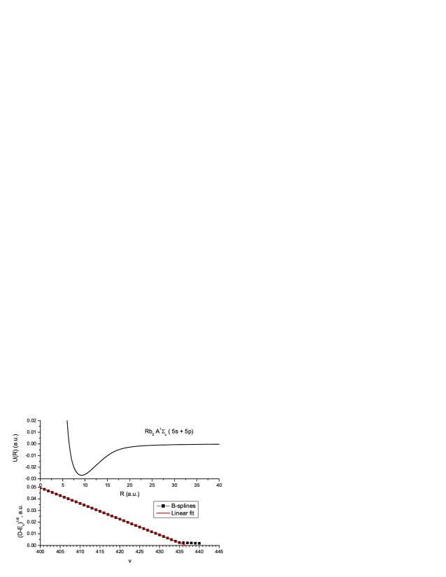
Figure 1: Upper panel: Molecular potential $A^{1}\Sigma_{u}^{+}$ of Rb₂ molecule. Lower panel: comparison of the Le Roy-Bernstein fit (solid line) with the results obtained with the B-spline code (squares).

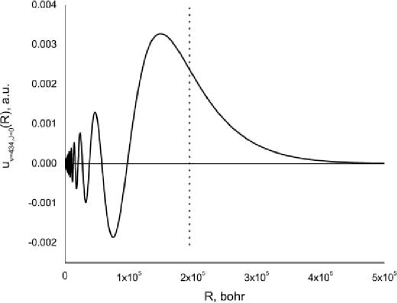
Figure 2: Vibrational wavefunction of $v=434,J=0$ level of the Rb $A^{1}\Sigma_{u}^{+}$ electronic potential as computed in the B-spline method. The vertical line marks the position of the classical turning point.

IV Relation between the position of the last bound level and the scattering length

Here we consider two atoms interacting at long-range separations via attractive $-C_{6}/R^{6}$, $C_{6}>0$, potentials. We will employ two scaling parameters: the van der Waals length $\bar{r}_{6}=\left(2\mu C_{6}\right)^{1/4}$ and energy $\bar{E}_{6}=1/\left(\mu\leavevmode\nobreak\ \left(\bar{r}_{6}\right)^{2}\right)$. In particular, the regime of quantum halo states is reached when the energy of the last bound state is $-E_{-1}\ll\bar{E}_{6}$ and its spatial extension reaches distances much larger than $\bar{r}_{6}$.

We have investigated the performance of the B-spline method in the case of a realistic molecular potential that follows the $1/R^{6}$ power law at large distances (this is the case of the ground state of the alkali dimers). The numerical results are quite similar to the already presented cases of the Morse and $1/R^{3}$ long-range potential. Instead, in this section we use the developed method to study universal relation between the scattering length and the position of the last bound state in the molecular potential. To this end we focus on a simple model of hard-core sphere with the van der Waals tail. In this model the short-range physics is modeled by placing an impenetrable wall at $R=R_{0}$:

$$V(R)=\left\{\begin{array}[c]{cc}\infty\,,&R<R_{0}\\ -C_{6}/R^{6}\,,&R\geq R_{0}\end{array}\right.\,.$$ (12)

This simple model offers insights into the universal laws of low-energy scattering. Let us enumerate several analytical results GriFla93 ; Gao04a for this model relevant to our discussion. These are formulated in terms of the scaling factor

$$\bar{a}=\frac{2\pi}{(\Gamma(1/4))^{2}}\bar{r}_{6}\approx 0.477989\,\bar{r}_{6},$$

and accumulated phase inside the potential

$$\Phi=\frac{\bar{r}_{6}^{2}}{2R_{0}^{2}}\,.$$

which determines the physics close to threshold. Indeed, the number of bound states is given by GriFla93

$$N_{b}=\lfloor\Phi/\pi-7/8\rfloor+1\,,$$

and the scattering length $a$ by GriFla93

$$a=\bar{a}\left(1-\tan(\Phi-3\pi/8)\right)\,.$$ (13)

For $|a|/r_{6}\gg 1$, there is either a bound level close to the dissociation limit ($a>0$) or a virtual state ($a<0$).

In our numerical study, we take $C_{6}=6851$ for the ground-state Cs dimer  DerJohSaf99 , and a reduced mass for ¹³³Cs atoms. For ¹³³Cs₂ molecule $\bar{r}_{6}\approx 202\leavevmode\nobreak\ a_{0}$, and $\bar{E}_{6}\approx 4.4\times 10^{-5}\leavevmode\nobreak\ \mathrm{cm}^{-1}$. Increasing $R_{0}$, the position of the inner “hard” wall of the potential, reduces the number of bound states in the potential. For example, we find from analytical formula that a new bound state appears at the value of $R^{*}_{0}\approx 6.02073$ a₀. The potential binds 180 states for $R_{0}$ just below $R^{*}_{0}$ and 179 states for $R_{0}$ just above $R^{*}_{0}$.

For our initial numerical test we choose the position of the inner wall at $R_{0}=6.02$ bohr. B-spline method reliably produces all 179 bound states and reveals a loosely bound state with the energy of $-9.33\times 10^{-12}$ a.u. We verified that the energies of the states near the dissociation limit follow the Le Roy-Bernstein pattern (similar to the analysis presented in Fig. 1 for the $1/R^{3}$ potential.) In this case, however, some additional observations can be made.

For $R_{0}=6.02$ a₀, the scattering length, Eq. (13) is large and positive, $a=+796$ a₀. Large and positive scattering lengths result from having a bound state just below the threshold. In this regime, the energy of the last bound state may be approximated by Gao04a

$$E_{-1}^{\mathrm{QDT}} \approx -\frac{1}{2\mu}\frac{1}{(a-\bar{a})^{2}}\times$$ (14)

$$\left(1+c_{1}\frac{\bar{r}_{6}}{(a-\bar{a})}+c_{2}\frac{\bar{r}_{6}^{2}}{(a-\bar{a})^{2}}\right)\,,$$

where $c_{1}\approx 0.4387552$, $c_{2}\approx-0.2163139$. The above expression was derived using the quantum defect theory and it substantially differs from the commonly-used effective range expansion formula

$$E_{-1}^{\mathrm{eff}}=-\frac{1}{2\mu}\frac{1}{a^{2}}\,.$$ (15)

From Eq. (14), we find $E_{-1}^{\mathrm{QDT}}\approx-9.35\times 10^{-12}$, while the effective-range formula results in $E_{-1}^{\mathrm{eff}}\approx-6.52\times 10^{-12}$. Clearly, our numerical result, $-9.33\times 10^{-12}$ a.u., supports the analytical analysisGao04a . In this calculation, the parameters of the grid were chosen to be $R_{\min}=R_{0}$, $R_{\max}=5\times 10^{4},\beta=0.4$, with the number of points 2407. When the number of points was reduced by a factor of 3, the energy of the last bound state was affected in the third significant figure. We again notice that the DVR method was unable to match the numerical accuracy of the B-spline approach.

While offering an improved accuracy over the effective-range expression, the QDT Eq.(14) is still an approximate result. In Fig. 3, we compare the QDT prediction with our numerical results. Here we move the position of the inner wall just below the critical value of $R^{*}_{0}\approx 6.02073$, at which the least bound state disappears. The range of the values for the position of the inner wall was chosen so that the scattering length remained positive. An increase in $R_{0}$ translates into increasingly larger values of the scattering length. For $a/\bar{a}\gg 1$, i.e., near the threshold, both the effective-range and the QDT results become identical. As the scattering length decreases, the effective range approximation rapidly loses its accuracy. Our comparison in Fig. 3 clearly demonstrates that, compared to the conventional effective-range theory, the QDT approximation is applicable over a much wider range of parameters. At the same time, as $R_{0}$ is decreased from its critical value, the QDT approximation starts to break down at $R_{0}\approx 6.017$ bohr. The relevant parameter governing the validity of Eq.(14) is the reduced scattering length $a/\bar{a}$: the critical value $R_{0}\approx 6.017$ a₀ corresponds to $a/\bar{a}\approx 2$. To reiterate, the QDT formula, Eq.(14), is an excellent approximation as long as $a/\bar{a}>2$, while the effective range approximation requires $a/\bar{a}\gg 1$.

Finally, it is worth pointing out that our method is robust enough to reproduce halo states of diatomic molecules bound by the van der Waals forces. We varied $R_{0}$ just below the threshold value and examined the energies of the least bound state produced by the B-spline method. For example, for $R_{0}=6.0207$, we obtain with the B-spline code $E_{-1}=-1.71\times 10^{-14}$ a.u., while analytical results are $E_{-1}^{\mathrm{QDT}}\approx-1.82\times 10^{-14}$ a.u. and $E_{-1}^{\mathrm{eff}}\approx-1.78\times 10^{-14}$ a.u. The binding energies are four orders of magnitude smaller than the van der Waals energy. At the same time, the corresponding scattering length, governing the extent of the wavefunction, is about $2\times 10^{4}$ bohr, i.e., two orders of magnitude larger than the van der Waals length. Satisfying both enumerated conditions signifies reaching the universal regime of quantum halo states.

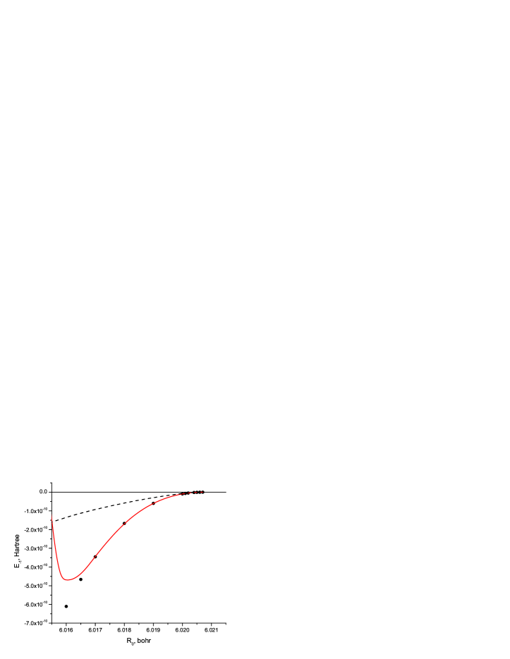
Figure 3: Energy of the last bound state as a function of the position of the inner wall of the model potential. Dots mark numerical results obtained with the B-spline approach. Predictions of the effective-range approximation are shown with a dashed line and that of the quantum-defect theory – with a solid line.

V Conclusion

With the experimental control of quantum-mechanical systems becoming more refined, new theoretical tools have to be adopted to meet the new challenges. Recently, fragile Feshbach (quantum halo-state) molecules became an experimental reality (see e.g., Ref. MarFerKoo07 ). Motivated by this progress, here we developed a numerical method for solving the Schrödinger equation for diatomic molecules based on the B-spline finite basis sets. The method produces a numerically complete quasi-spectrum of rovibrational states. We find, that B-splines offer an accurate description of the loosely-bound molecular states near the dissociation limit. The quasi-spectrum is entirely devoid of the unphysical ghost states which appear in DVR method and require special effort to be eliminated WilDulMas04 ; kallush2006 . Moreover, coupled with the “mapped grid” method of Ref. WilDulMas04 , the representation is both accurate and efficient: both rapidly-oscillating part of the wavefunction in the classically-allowed region and the slowly-varying exponential tail in the classically-forbidden region are adequately reproduced. As an application of the developed method we investigated the universal law relating the energy of the last bound state to the scattering length. We find that the new QDT formulation of such a law for $1/R^{6}$ potentials by Gao Gao04a remains valid over a substantially wider range of parameters than the commonly-used effective-range approximation.

References

- (1) Ernest Davidson and David Feller. Basis set selection for molecular calculations. Chem. Rev., 86:681 – 696, 1986.
- (2) W. R. Johnson, S. A. Blundell, and J. Sapirstein. Finite basis sets for the Dirac equation constructed from B–splines. Phys. Rev. A, 37(2):307–15, 1988.
- (3) H Bachau, E Cormier, P Decleva, J. E. Hansen, and F Martin. Applications of B-splines in atomic and molecular physics. Rep. Prog. Phys., 64:1815–1943, 2001.
- (4) Bruce W. Shore. Solving the radial Schrodinger equation by using cubic-spline basis functions. J. Chem. Phys., 58(9):3855–3866, 1973.
- (5) V. Kokoouline, O. Dulieu, R. Kosloff, and F. Masnou-Seeuws. Mapped Fourier methods for long range molecules: Application to perturbations in the Rb) spectrum. J. Chem. Phys., 110:9865, 1999.
- (6) K. Willner, O. Dulieu, and F. Masnou-Seeuws. Mapped grid methods for long-range molecules and cold collisions. J. Chem. Phys, 120:57–64, 2004.
- (7) F. Masnou-Seeuws and P. Pillet. Formation of ultracold molecules (t¡ 200 K) via photoassociation in a gas of laser-cooled atoms. Adv. At. Mol. Phys., 47:53–127, 2001.
- (8) J. Doyle, B. Friedrich, R. Krems, and F. Masnou-Seeuws. Quo vadis, cold molecules. Eur. Phys. J. D, 31:149–164, december 2004.
- (9) A. Crubellier, O. Dulieu, F. Masnou-Seeuws, M. Elbs, H.Knöckel, and E. Tiemann. Simple determination of Na2 scattering lengths using observed bound levels at the ground state asymptote. Eur. Phys. J. D, 6:211, 1999.
- (10) Thorsten Köhler, Krzysztof Góral, and Paul S. Julienne. Production of cold molecules via magnetically tunable Feshbach resonances. Rev. Mod. Phys., 78(4):1311, 2006.
- (11) A. S. Jensen, K. Riisager, D. V. Fedorov, and E. Garrido. Structure and reactions of quantum halos. Rev. Mod. Phys., 76(1):215, 2004.
- (12) C. Koch, José Palao, R. Kosloff, and F. Masnou-Seeuws. How to obtain ultracold =0 molecules using optimal control theory. Phys. Rev. A, 70:013402, 2004.
- (13) Avi Pe’er, Evgeny A. Shapiro, Matthew C. Stowe, Moshe Shapiro, and Jun Ye. Precise control of molecular dynamics with a femtosecond frequency comb. Phys. Rev. Lett., 98(11):113004, 2007.
- (14) L. D. Landau and E. M. Lifshitz. Quantum Mechanics, volume III. Butterworth-Heinemann, 3 edition, 1997.
- (15) Bo Gao. Binding energy and scattering length for diatomic systems. J. Phys. B, 37(21):4273–4279, 2004.
- (16) Carl de Boor. A practical guide to splines. Springer-Verlag, New York, revised edition, 2001.
- (17) W. R. Johnson. Atomic Structure Theory: Lectures on Atomic Physics. Springer, New York, NY, 2007.
- (18) R. Kosloff. Quantum molecular Dynamics on Grids. In R. H. Wyatt and J. Z. H. Zhang, editor, Dynamics of Molecules and Chemical Reactions, page 185. Marcel Dekker, New York, 1996.
- (19) David Gottlieb and Steven A. Orszag. Numerical analysis of spectral methods: Theory and applications. CBMS-NSF Regional Conference Series in Applied Mathematics, No. 26. Society for Industrial and Applied Mathematics, Philadelphia, Pa., 1977.
- (20) V. Kokoouline, O. Dulieu, and F. Masnou-Seeuws. Theoretical treatment of channel mixing in excited Rb2 and Cs2 ultra-cold molecules. perturbations in photoassociation and fluorescence spectra. Phys. Rev. A, 62:022504, 2000.
- (21) V. Kokoouline, O. Dulieu, R. Kosloff, and F. Masnou-Seeuws. Theoretical treatment of channel mixing in excited Rb2 and Cs2 ultra-cold molecules : determination of predissociation lifetimes with coordinate mapping. Phys. Rev. A, 62:032716, 2000.
- (22) R. J. Le Roy and R. B. Bernstein. J. Chem. Phys., 52:3869, 1970.
- (23) P. H. Morse. Diatomic molecules according to the wave mechanics. II. Vibrational levels. Phys. Rev., 34:57–64, 1929.
- (24) R Shakeshaft. Low energy scattering by the r-3 potential. J. Phys. B, 5(6):L115–L117, 1972.
- (25) C. Boisseau, E. Audouard, J. Vigué, and V.V. Flambaum. Analytical correction to the WKB quantization condition for the highest levels in a molecular potential. Eur. Phys. J. D, 12:199–209, 2000.
- (26) G. F. Gribakin and V. V. Flambaum. Calculation of the scattering length in atomic collisions using the semiclassical approximation. Phys. Rev. A, 48(1):546–553, 1993.
- (27) A. Derevianko, W. R. Johnson, M. S. Safronova, and J. F. Babb. High-precision calculations of dispersion coefficients, static dipole polarizabilities, and atom-wall interaction constants for alkali-metal atoms. Phys. Rev. Lett., 82(18):3589–92, 1999.
- (28) M. Mark, F. Ferlaino, S. Knoop, J. G. Danzl, T. Kraemer, C. Chin, H.-C. Nägerl, and R. Grimm. Spectroscopy of ultracold trapped cesium Feshbach molecules. Phys. Rev. A, 76(4):042514, 2007.
- (29) S. Kallush and R. Kosloff. Improved methods for mapped grids: Applied to highly excited vibrational states of diatomic molecules. Chem. Phys. Lett., 433:231, 2006.