Self-similar planar graphs as models for complex networks

Abstract

In this paper we introduce a family of planar, modular and self-similar graphs which have small-world and scale-free properties. The main parameters of this family are comparable to those of networks associated to complex systems, and therefore the graphs are of interest as mathematical models for these systems. As the clustering coefficient of the graphs is zero, this family is an explicit construction that does not match the usual characterization of hierarchical modular networks, namely that vertices have clustering values inversely proportional to their degrees.

1 Introduction

Research and studies performed in the last few years show that many networks associated with complex systems, like the World Wide Web, the Internet, telephone networks, transportation systems (including power and water distribution networks), social and biological networks, belong to a class of networks now known as small-world scale-free networks, see [1, 11] and references therein. These networks exhibit a small average distance and diameter (with respect to a random network with the same number of nodes and links) and, in many cases, a strong local clustering (nodes have many mutual neighbors). Another important common characteristic is that the number of links attached to the nodes usually obeys a power-law distribution (is scale-free). By introducing a new measuring technique, it has recently been discovered that many real networks are also self-similar, see [15, 16]. Moreover, a degree hierarchy in these networks is sometimes related to the modularity of the system which they model.

Most of the network models considered are probabilistic, however in recent years some deterministic models have been proposed which are very often based on iterative constructions such that, at each step, one or more vertices are connected to certain subgraphs (for example, the so called $k$-trees [4]). Another technique produces graphs by duplication of certain substructures, see [5]. Here we propose a new family of graphs which generalize these methods by introducing at each iteration a more complex substructure than a single vertex. The result is a family of planar, modular, hierarchical and self-similar graphs, with small-world scale-free characteristics and with clustering coefficient zero. We note that some important real life networks, for example the networks associated to electronic circuits or Internet [11], have these characteristics as they are modular, almost planar and with a reduced clustering coefficient and have small-world scale-free properties. Thus, these networks can be modeled by our construction. A related family of graphs based on triangles, and which therefore has a high clustering coefficient was introduced in [19].

2 Hierarchical modular graphs

Several authors classify as hierarchical graphs, graphs with a modular structure and a strong connectedness hierarchy of the vertices which produces a power-law degree distribution. Moreover, they consider that the most important signature of hierarchical modularity is given by a clustering distribution with respect to the degree according to $C(k)\propto 1/k$, see [2, 8, 17]. In this section we define an analyze a family of hierarchical modular graphs, which are scale-free, planar and have clustering coefficient zero. They prove the existence of hierarchical graphs which do not have the above-mentioned relationship between the clustering coefficient and the degrees of the corresponding vertices.

Deterministic models for simple hierarchical networks have been published in [12, 13]. These models consider the recursive union of several basic structures (in many cases, complete graphs) by adding edges connecting them to a selected root vertex. These and other hierarchical graphs have been considered when modeling metabolic networks in [10, 14]. Hierarchical modularity also appears in some models based on $k$-trees or clique-trees, where the graph is constructed by adding at each step one or more vertices and each is connected independently to a certain subgraph [8, 6, 18]. The introduction of the so-called hierarchical product of graphs in [7] allows a generalization and a rigorous study of some of these models.

In [15, 16], Song, Havlin and Makse relate the scale-free and the self-similarity properties as they verify that many self-similar graphs associated to real life complex systems have a fractal dimension and provide a connection between this dimension and the exponent of the degree power-law. However, a classical scale-free mode, the preferential attachment by Bar basi-Albert [1], which many authors consider a paradigm for these networks, has a null fractal dimension. This is not a paradox as the Barabási-Albert model lacks modularity because of its generation process based on the individual introduction of vertices.

In the next subsection we give details of our construction which is also based on an iterative process. However, the introduction at each step of a certain substructure allows the formation of modules and results in a final graph with a self-similar structure.

2.1 Iterative algorithm to generate the graph $H(t)$

The graph $H(t)$ is constructed as follows: For $t=0$, $H(0)$ is $C_{4}$, a length four cycle. We define now as generating cycle a cycle $C_{4}$ whose vertices have not been introduced at the same iteration step and passive cycle a cycle $C_{4}$ which does not verify this property. For $t\geq 1$, $H(t)$ is obtained from $H(t-1)$ by considering all their generating cycles $C_{4}$ and connecting, vertex to vertex, to each of them a new cycle $C_{4}$. This operation is equivalent to adding to the graph a cube $Q_{3}$ by identifying vertex to vertex the generating cycle with one of the cycles of $Q_{3}$. The process is repeated until the desired graph order is reached.

Figure 1: Graphs $H(t)$ produced at iterations $t=1,2$ and $3$.

2.2 Recursive modular construction

The graph $H(t)$ can be also defined as follows: For $t=0$, $H(0)$ is the cycle $C_{4}$. For $t\geq 1$, $H(t)$ is produced from four copies of $H(t-1)$ by identifying, vertex to vertex, the initial passive cycle of each $H(t-1)$ with each of four consecutive cycles of $Q_{3}$ (leaving two opposite cycles of $Q_{3}$ free), see Fig. 2.

Figure 2: Modular construction of $H(t)$ for $t=1,2$ y $3$. At step $t$, we merge four copies of $H(t-1)$ to four cycles of the cube $Q_{3}$, leaving opposite cycles free. See the text for details.

2.3 Properties of $H(t)$

Order and size of $H(t)$.— We use the following notation: $\tilde{V}(t)$ and $\tilde{E}(t)$ denote, respectively, the set of vertices and edges introduced at the step $t$ and $\tilde{C}(t)$ is the number of generating cycles $C_{4}$ at this step (which will be used to produce the graph $H(t+1)$.

Note that at each iteration, any generating cycle is replaced by four new generating cycles and one passive cycle. Therefore: $\tilde{C}(t+1)=4\cdot\tilde{C}(t),t\geq 1$ and $\tilde{C}(0)=1$. Thus $\tilde{C}(t)=4^{t}$. Moreover, each generating cycle introduces at the next iteration four new vertices and eight new edges. As a consequence, $\tilde{V}(t)=4\cdot\tilde{C}(t-1)=4\cdot 4^{t-1}$ and $\tilde{E}(t)=8\cdot\tilde{C}(t-1)=8\cdot 4^{t-1}=2\cdot 4^{t}$, thus:

$$|V(t)|=\sum_{i=0}^{t}\tilde{V}(t)=\frac{4^{t+1}+8}{3}\qquad|E(t)|=\sum_{i=0}^{t}\tilde{E}(t)=\frac{2\cdot 4^{t+1}+4}{3}$$

Step	Vertices	Edges	Number of active cycles
0	4	4	1
1	8	12	4
2	24	44	16
3	88	172	64
$\cdots$	$\cdots$	$\cdots$	$\cdots$
t	$\frac{4^{t+1}+8}{3}$	$\frac{2\cdot 4^{t+1}+4}{3}$	$4^{t}$
$\cdots$	$\cdots$	$\cdots$	$\cdots$

Table 1: Number of vertices, edges and generating cycles of $H(t)$ at each step.

Degree distribution.— Intially, at $t=0$, the graph is a single generating cycle $C_{4}$ and its four vertices have degree two.

When a new vertex $i$ is added to the graph at iteration $t_{i}$ ($t_{i}\geq 1$), it has degree $3$. We denote by $C(i,t)$ the number of generating cycles at iteration $t$ which will produce new vertices that will connect to vertex $i$ at step $t+1$. At iteration $t_{i}$, when vertex $i$ is introduced, the value of $C(i,t_{i})$ is $2$. According to the construction process of the graph, at each iteration, each new neighbor of $i$ belongs to two generating cycles where $i$ is also a vertex. If we denote as $k(i,t)$ the degree of vertex $i$ at step $t$, then we have the following relationship: $C(i,t)=k(i,t)-1$.

We now compute $C(i,t)$. As we have seen above, each generating cycle where $i$ belongs to, produces two new generating cycles which also have $i$ as a vertex. Thus $C(i,t)=2\cdot C(i,t-1)$. Using the initial condition $C(i,t_{i})=2$, we have $C(i,t)=2^{t-t_{i}+1}$. Therefore the degree of vertex $i$ at the step $t$ is

$$k(i,t)=2^{t-t_{i}+1}+1.$$ (1)

Note that the initial four vertices of step 0 follow a different process. In this case $C(i,0)=2^{t}$ and $k(i,t)=2^{t}+1$. Thus, at step $t$ the initial four vertices of the graph have the same degree than those introduced at step 1.

From equation (1) we verify that the graph has a discrete degree distribution and we use the technique described by Newman in  [11] to find the cumulative degree distribution $P_{\rm cum}(k)$ for a vertex with degree $k$: $P_{\rm cum}(k)=\sum_{\tau\leq t_{i}}{|V(\tau)|}/{|V(t_{i})|}=({4^{t_{i}+1}+8)/(4^{t+1}+8})$.

Replacing $t_{i}$, from equation (1), in the former equation $t_{i}=t+1-{\ln(k-1)}/{\ln 2}$ we obtain $P_{\rm cum}(k)=({16\cdot 4^{t}\cdot(k-1)^{-2}+8})/({4^{t}+8})$, which for large values of $t$, allows us to write $P_{\rm cum}(k)\sim k^{1-\gamma_{k}}=k^{-2}$, and therefore the degree distribution, for large graphs, follows a power-law with exponent $\gamma_{k}=3$. Research on networks associated to electronic circuits (these networks show planarity, modularity and a small clustering coefficient) gives similar values for their degree power-law distribution [9, 11]. More precisely, the largest benchmark considered –a network with 24097 nodes, 53248 edges, average degree 4.34 and average distance 11.05– has a degree distribution which follows a power-law with exponent 3.0, precisely the same as in our model, and it has a small clustering coefficient $C=0.01$.

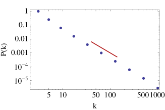
Figure 3: Log-log representation of the cumulative degree distribution for $H(10)$ with $|V|=1398104$ vertices. The reference line has slope $-2$.

Diameter.— At each step we introduce, for each generating cycle, four new vertices which will form a new cycle $C_{4}$ (and these vertices are among them at maximum distance 2). As all join the graph of the former step with one new edge, in the worst situation the diameter will increase by exactly 2 units. Therefore $D_{t}=D_{t-1}+2$. $t\geq 2$. As $D_{1}=3$, we have that the diameter of $H(t)$ is $D_{t}=2\cdot t+1$ if $t\geq 1$.

Average distance.— The average distance of $H(t)$ is defined as:

$$\bar{d}_{t}=\frac{1}{{\mbox{\scriptsize$|V(t)|(|V(t)|-1)/2$}}}\sum_{i,j\in V(t)}d_{i,j}\,,$$ (2)

where $d_{i,j}$ is the distance between vertices $i$ and $j$. We will denote as $S_{t}$ the sum $\sum_{i,j\in V(t)}d_{i,j}$.

The modular recursive construction of $H(t)$ allows us to calculate the exact value of $\bar{d}_{t}$. At step $t$, $H(t+1)$ is obtained from the juxtaposition of four copies of $H(t)$, which we label $H_{t}^{\varphi}$, $\varphi=1,2,3,4$, on top of the cube $Q_{3}$ (see Figs. 2 and 4). The copies are connected one to another at the vertices which we call connecting vertices and we label $w$, $x$, $y$, $z$, $o$, $r$, $s$, and $a$. The other vertices of $H(t+1$ will be called interior vertices. Thus, the sum of distances distance $S_{t+1}$ satisfies the following recursion:

$$S_{t+1}=4\,S_{t}+\Delta_{t}-4.$$ (3)

where $\Delta_{t}$ is the sum over all shortest paths whose endvertices are not in the same $H(t)$ copy and the last term compensates for the overcounting of some paths between the connecting vertices –for example, $d(w,o)$ is included both in $H_{t}^{1}$ and $H_{t}^{2}$–. Note that the paths that contribute to $\Delta_{t}$ must all go through at least one of the eight connecting vertices. The analytical expression for $\Delta_{t}$ is not difficult to find.

Figure 4: Illustration of the classification of nodes in $H_{t}^{\varphi}$, $\varphi=1,2,3,4$.

We denote as $\Delta_{t}^{\alpha,\beta}$ the sum of all shortest paths with endvertices in $H_{t}^{\alpha}$ and $H_{t}^{\beta}$. $\Delta_{t}^{\alpha,\beta}$ excludes the paths such that either endvertex is a connecting vertex. Then the total sum $\Delta_{t}$ is

$$\Delta_{t} = \Delta_{t}^{1,2}+\Delta_{t}^{1,3}+\Delta_{t}^{1,4}+\Delta_{t}^{2,3}+\Delta_{t}^{2,4}+\Delta_{t}^{3,4}+20$$ (4)

$$+\sum_{\stackrel{{\scriptstyle i\in H_{t}^{3}\cup H_{t}^{4},}}{{i\notin x,r,s,y,a,z}}}(d_{w,i}+d_{o,i})+\sum_{\stackrel{{\scriptstyle i\in H_{t}^{1}\cup H_{t}^{4},}}{{i\notin w,o,a,z,s,y}}}(d_{x,i}+d_{r,i})$$

$$+\sum_{\stackrel{{\scriptstyle i\in H_{t}^{1}\cup H_{t}^{2},}}{{i\notin x,r,o,w,a,z}}}(d_{s,i}+d_{y,i})+\sum_{\stackrel{{\scriptstyle i\in H_{t}^{2}\cup H_{t}^{3},}}{{i\notin w,o,x,r,s,y}}}(d_{a,i}+d_{z,i}),$$

where the term 20 comes from the sum of $d_{w,s}$, $d_{w,y}$, $d_{o,s}$, $d_{o,y}$, $d_{x,a}$, $d_{x,z}$, $d_{r,a}$, and $d_{r,z}$.

By symmetry, $\Delta_{t}^{1,2}=\Delta_{t}^{1,4}=\Delta_{t}^{2,3}=\Delta_{t}^{3,4}$, $\Delta_{t}^{1,3}=\Delta_{t}^{2,4}$, and $\sum_{i}d_{w,i}=\sum_{i}d_{o,i}=\sum_{i}d_{x,i}=\sum_{i}d_{r,i}=\sum_{i}d_{s,i}=\sum_{i}d_{y,i}=\sum_{i}d_{a,i}=\sum_{i}d_{z,i}$, and

$$\Delta_{t}=4\Delta_{t}^{1,2}+2\Delta_{t}^{1,3}+8\,\sum_{\stackrel{{\scriptstyle i\in H_{t}^{3}\cup H_{t}^{4},}}{{i\notin x,r,s,y,a,z}}}d_{w,i}\,.$$ (5)

To calculate $\Delta_{t}$, we classify the interior vertices of $H(t+1)$ into four different classes according to their distances to each of the four vertices $w$, $x$, $y$, and $z$. Vertices $w$, $x$, $y$, and $z$ are not classified into any of these classes which we represent as $P_{1}$, $P_{2}$, $P_{3}$, and $P_{4}$, respectively. This classification is represented in Fig. 4. By construction, for an arbitrary interior vertex $v$, there must exist one of the above mentioned vertices (say $w$) satisfying $d_{v,w}<d_{v,x}$, $d_{v,w}<d_{v,y}$, and $d_{v,w}<d_{v,z}$. All the interior vertices nearest to $w$ (resp. $x$, $y$, and $z$) are assigned to class $P_{1}$ (resp. $P_{2}$, $P_{3}$, and $P_{4}$). The total number of vertices of $H_{t}$ that belong to the class $P_{\tau}$ ($\tau=1,2,3,4$) is denoted by $N_{t,P_{\tau}}$. Since the four vertices $w$, $x$, $y$, and $z$ play a symmetrical role, classes $P_{1}$, $P_{2}$, $P_{3}$, and $P_{4}$ are equivalent. Thus, $N_{t,P_{1}}=N_{t,P_{2}}=N_{t,P_{3}}=N_{t,P_{4}}$ which will be abbreviated to $N_{t}$ from now on. We have

$$N_{t}=\frac{|V_{t}|-4}{4}=\frac{4^{t}-1}{3}.$$ (6)

We denote by $L_{t+1,P_{1}}$ ($L_{t+1,P_{2}},L_{t+1,P_{3}},L_{t+1,P_{4}}$) the sum of distances between vertices $w$ ($x$, $y$, $z$) and all interior vertices $v\in P_{1}$ $(P_{2},P_{3},P_{4})$ of $H(t+1)$. Because of the symmetry, $L_{t+1,P_{1}}=L_{t+1,P_{2}}=L_{t+1,P_{3}}=L_{t+1,P_{4}}$ that will be written as $L_{t+1}$ for short. Taking into account the second method of constructing $H(t)$, see Fig. 4, we can write the following recursive formula for $L_{t+1}$:

$$L_{t+1}=4\,L_{t}+2\,N_{t}+1.$$ (7)

We can solve Eq. (7) inductively, with initial condition $L_{1}=1$, and we have

$$L_{t}=\frac{1}{18}\left(3t\cdot 4^{t}+2\cdot 4^{t}-2\right).$$ (8)

We now return to compute Eq. (5), with $\Delta_{t}^{1,2}$ given by the sum

$$\Delta_{t}^{1,2}=\!\!\sum_{\stackrel{{\scriptstyle u\in H_{t}^{1},u\notin\{w,o,a,z\};}}{{\,v\in H_{t}^{2},v\notin\{w,x,r,o\}}}}\!\!\!d_{u,v}=\sum_{i=1}^{4}\sum_{j=1}^{4}d_{P^{t,1}_{i},P^{t,2}_{j}}\,,$$ (9)

where $P^{t,1}_{i}$ and $P^{t,2}_{j}$ are the vertex classes $P_{i}$ and $P_{j}$ of $H_{t}^{1}$ and $H_{t}^{2}$, respectively, and $d_{P^{t,1}_{i},P^{t,2}_{j}}$ is the sum of distances $d_{u,v}$ for all vertices $u\in P_{i}\subset H_{t}^{1}$ and $v\in P_{j}\subset H_{t}^{2}$.

We have:

$$d_{P^{t,1}_{1},P^{t,2}_{1}}=\!\!\sum_{\stackrel{{\scriptstyle u\in P_{1}\subset H_{t}^{1},}}{{\,v\in P_{1}\subset H_{t}^{2}}}}\!\!d_{u,v}=\!\!\sum_{\stackrel{{\scriptstyle u\in P_{1}\subset H_{t}^{1},}}{{\,v\in P_{1}\subset H_{t}^{2}}}}\!\!(d_{u,o}+d_{o,r}+d_{r,v})=2N_{t}L_{t}+N_{t}^{2}.$$ (10)

Following the same process, we obtain $d_{P^{t,1}_{i},P^{t,2}_{j}}$ for the different values of $i$ and $j$, which we use in Eq. (9) giving:

$$\Delta_{t}^{1,2}=32\,N_{t}L_{t}+24\,(N_{t})^{2}\,.$$ (11)

Analogously, we can obtain

$$\Delta_{t}^{1,3}=32\,N_{t}L_{t}+32\,(N_{t})^{2}\,.$$ (12)

Now, to find an expression for $\Delta_{t}$, the only thing left is to evaluate the last term of Eq. (5), which can be obtained as above

$$8\!\!\!\sum_{\stackrel{{\scriptstyle i\in H_{t}^{3}\cup H_{t}^{4}\,,}}{{i\notin x,r,s,y,a,z}}}\!\!d_{w,i}=64\,L_{t}+128\,N_{t}\,.$$ (13)

Finally, and combining the former expressions, we write the exact result for the average distance of $H(t)$, $\bar{d}_{t}$, as

$$\bar{d}_{t}=\frac{4}{3}\cdot\frac{10+14\cdot 4^{t}+3(t+1)16^{t}}{10+13\cdot 4^{t}+4\cdot 16^{t}}\,.$$ (14)

Notice that for a large order ($t\rightarrow\infty$) $\bar{d}_{t}\simeq t+1\sim\ln|V_{t}|$, which means that the average distance shows a logarithmic scaling with the order of the graph, and has a similar behavior as the diameter (the graph is small-world).

Strength distribution.— The strength of a node in a network is associated to resources or properties allocated to it, as the total number of publication of an author, in the case of the network associated to the Erdős number; the total number of passengers in the world-wide airports network, etc.

In our case we associate to each vertex the area of the passive cycle, defined by the four vertices introduced at a given step. For this purpose we assume a uniform construction of the graph. At the initial step the area is ${\cal{A}}_{0}$ and we denote as ${\cal{A}}_{t}$ the area of the passive cycle introduced at step $t$. By convention, we establish that the area of this cycle is one fifth of the area of the cycle where it connects (as each introduction of a passive cycle is associated to the simultaneous introduction of four generating cycles). Therefore we have ${\cal{A}}_{t}=(\frac{1}{5})^{t}{\cal{A}}_{0}$. A vertex $i$ introduced at $t_{i}$ will have strength $s(i,t_{i})=(\frac{1}{5})^{t_{i}}{\cal{A}}_{0}$ and it will keep it i n further steps $t>t_{i}$. As we want to find the strength distribution for all vertices of the graph at step $t$, we have that $s(i,t_{i})=(\frac{1}{5})^{t_{i}-t}\cdot{\cal{A}}_{t}$.

Using equation (1) we obtain the following power-law for the correlation between the strength and the degree of a vertex:

$$s(i,t)=\frac{1}{5}{\cal{A}}_{t}(k(i,t)-1)^{\ln 5/\ln 3},$$ (15)

which for large values of the degree $k$ leads to $s(k)\sim k^{\ln 5/\ln 3}$.

We should mention that similar exponents have been found for the relation between the strength and the degree of the node of real life networks like the airports network, Internet and the scientist collaboration graph [3].

After a similar analysis to the calculation of the degree distribution, we find that the strength distribution also follows a power law with exponent:

$$\gamma_{s}=1+2\frac{\ln 2}{\ln 5}.$$ (16)

It has been shown that if a weighted graph with a non-linear correlation between strength and degree $s(k)\sim k^{\beta}$ and the degree and strength distributions follows power laws, $P(k)\sim k^{-\gamma_{k}}$ and $P(s)\sim s^{-\gamma_{s}}$, then there exists a general relationship between $\gamma_{k}$ y $\gamma_{s}$ given by $\gamma_{s}=\frac{\gamma_{k}}{\beta}+\frac{\beta-1}{\beta}$  [3].

As in our case $\gamma_{k}=3$ y $\beta={\ln 5/\ln 3}$ from the former relationship, the exponent of the strength distribution is $\gamma_{s}=3\frac{\ln 2}{\ln 3}+\ln 2({\frac{\ln 5}{\ln 2}-1})/{\ln 5}$, and we obtain the same value $\gamma_{s}$ (16) which was computed directly.

3 Conclusion

The family of graphs introduced and studied here has as main characteristics planarity, modularity, degree hierarchy, and small-world and scale-free properties. At the same time the graphs have clustering zero. A combination of modularity and scale-free properties is present in many real networks like those associated to living organism (protein-protein interaction networks) and some social and technical networks [13, 14]. The added property of a small clustering coefficient appears also in some technological networks (electronic circuits, Internet, P2P) and social networks [11]. Therefore our model, with a null clustering coefficient, could be considered to model these networks and also it can be used to study other properties without the influence of the clustering. The deterministic character of the family, as opposed to usual probabilistic models, should facilitate the exact computation of many network parameters.

On the other hand, simple variations of our model allow the introduction of clustering. As an example, by adding to each passive cycle an edge we can introduce two triangles for each cycle and therefore obtain a planar graph with non-zero clustering. Replacing in the construction each passive cycle by a complete graph $K_{4}$ will produce a family with a relatively large clustering coefficient. However the graph will no longer be planar.

References

- [1] R. Albert, A.-L. Barabási. Statistical mechanics of complex networks, Rev. Mod. Phys. 74:47–97, 2002.
- [2] A.-L. Barabási and Z.N. Oltvai, Network biology: Understanding the cell’s functional organization, Nature Rev Genetics 5:101–113, 2004.
- [3] A. Barrat, M. Barthélemy, R. Pastor-Satorras, A. Vespignani. Proc. Natl. Acad. Sci. U.S.A. 101: 3747, 2004.
- [4] L.W. Beineke, R.E. Pippert. Properties and characterization of k-trees. Mathematika 18:141–151, 1971.
- [5] F. Chung, L. Lu, T.G. Dewey, D.J. Galas. Duplication models for biological networks. J. Comput. Biol. 10(5):677–87, 2003.
- [6] F. Comellas, G. Fertin, A. Raspaud. Recursive graphs with small-world scale-free properties, Phys. Rev. E 69: 037104, 2004.
- [7] L. Barriere, F. Comellas, C.Dalf , M.A. Fiol. The hierarchical product of graphs. Discrete Appled Math. En prensa, 2008.
- [8] S.N. Dorogovtsev, A.V. Goltsev, J.F.F. Mendes. Pseudofractal scale-free web. Phys. Rev. E 65: 066122, 2002.
- [9] R. Ferrer i Cancho, C. Janssen, R.V. Solé Topology of technology graphs: Small world patterns in electronic circuits. Phys. Rev. E 64:046119, 2001.
- [10] H. Jeong, B. Tombor, R. Albert, Z.N. Oltvai, A.-L. Barabási. The large-scale organization of metabolic networks. Nature 407: 651–654, 2000.
- [11] M.E.J. Newman, The structure and function of complex networks, SIAM Review ,45:167–256, 2003 .
- [12] J.D. Noh, Exact scaling properties of a hierarchical network model, Phys. Rev. E 67:045103, 2003 .
- [13] E. Ravasz, A.-L. Barabási. Hierarchical organization in complex networks. Phys. Rev. E 67:026112, 2003 .
- [14] E. Ravasz, A. L. Somera, D. A. Mongru, Z. N. Oltvai, A.-L. Barabási. Hierarchical organization of modularity in metabolic networks. Science 297: 1551–1555, 2002.
- [15] C. Song, S. Havlin, H. A. Makse. Self-similarity of complex networks. Nature, 433:392–395, 2005.
- [16] C. Song, S. Havlin, H. A. Makse. Origins of fractality in the growth of complex networks. Nature Phys., 2:275–281, 2006.
- [17] S. Wuchty, E. Ravasz, A.-L. Barabási, “The Architecture of Biological Networks”, Complex Systems in Biomedicine, T.S. Deisboeck, J. Yasha Kresh and T.B. Kepler (Editors), Kluwer Academic Publishing, New York, 2003.
- [18] Z.Z. Zhang, F. Comellas, G. Fertin, and L.L. Rong. High dimensional Apollonian networks. J Phys A: Math Gen 39:1811–1818, 2006.
- [19] Z.Z. Zhang, S. Zhou, L. Fang, J. Guan, Y. Zhang. Maximal planar scale-free Sierpinski networks with small-world effect and power law strength-degree correlation. Europhys. Lett. 79:38007, 2007.