Distinguished trajectories in time dependent vector fields

Abstract

We introduce a new definition of distinguished trajectory that generalises the concepts of fixed point and periodic orbit to aperiodic dynamical systems. This new definition is valid for identifying distinguished trajectories with hyperbolic and non-hyperbolic types of stability. The definition is implemented numerically and the procedure consist in determining a path of limit coordinates. It has been successfully applied to known examples of distinguished trajectories. In the context of highly aperiodic realistic flows our definition characterises distinguished trajectories in finite time intervals, and states that outside these intervals trajectories are no longer distinguished.

Corresponding author: Ana M. Mancho, Instituto de Ciencias Matemáticas, Consejo Superior de Investigaciones Científicas, Serrano 121, 28006, Madrid. e-mail: A.M.Mancho@imaff.cfmac.csic.es. Phone: +34 91 5616800 ext 2408. Fax: +34 91 5854894.

This paper attempts to generalise the concepts of fixed point and periodic orbit to time dependent aperiodic dynamical systems. Fixed points and periodic orbits are keystones for describing solutions of autonomous and time periodic dynamical systems, as the stable and unstable manifolds of these hyperbolic objects form the basis of the geometrical template organising the description of the dynamical system. The mathematical theory of aperiodic dynamical systems is far from complete. In this context, this work deals with a general definition that encompasses the concepts of fixed point and periodic orbit and which when applied to finite time and aperiodic dynamical systems identifies special trajectories that play an organising role in the geometry of the flow.

1 Introduction

In recent years the theory of dynamical systems has provided a useful framework for describing transport in fluid flows. Since the seminal work by Aref [1] on chaotic advection much progress has been made both in theory and applications. Dynamical systems techniques were first applied to Lagrangian transport in the context of two-dimensional, time-periodic flows [2] and stationary 3D flows such as the ABC flow [3]. More recently these techniques have been extended to describe aperiodic flows [4, 7, 8] and finite time-dependent flows, such as those rising in geophysical applications [11, 12]. However, the mathematical theory for both aperiodic time-dependent flows and finite time aperiodic flows is far from being completely developed.

For stationary flows the idea of fixed point is a key for describing geometrically the solutions. Fixed points may be classified as hyperbolic or non-hyperbolic depending on their stability properties. Stable and unstable manifolds of hyperbolic fixed points organise the phase portraits of the flow away from the region close to the fixed points [5, 6]. These manifolds comprise respectively the trajectories that approach the fixed points as time tends to plus or minus infinite. As they are formed of trajectories they act as barriers to transport as particles cannot cross them without violating the uniqueness of the solution. They are useful because they allow qualitative predictions for the evolution of sets of initial conditions avoiding explicit integration of initial conditions on the whole domain. Hyperbolic fixed points and their stable and unstable manifolds are the basic notions used for the geometrical description of flows in autonomous dynamical system.

The concept of fixed point is extended to time periodic flows by means of the Poincaré map, as periodic orbits with period $T$ become fixed points of the Poincaré map. For hyperbolic periodic orbits there exist also stable and unstable manifolds that are geometric objects that organise the global dynamics. Again they are respectively the sets of orbits asymptotically approaching the periodic orbit as time tends to plus or minus infinity.

Aperiodic flows are still poorly understood, as theory that is well established for autonomous or periodic flows does not apply to them directly. For instance there exists efforts in the mathematical community to extend the well known concept of bifurcation for stationary flows to non-autonomous systems [9, 10]. To gain insight on the geometrical structure of aperiodic flows, concepts such as Lyapunov exponents are used, however these are defined strictly on infinite time systems. Realistic flows, like those arising in geophysics or oceanography, are not infinite time systems and for their description, finite time versions of the definition of Lyapunov exponents such as Finite Size Lyapunov Exponents (FSLE) [14] and Finite Time Lyapunov Exponents (FTLE) [15, 16] are used. Special trajectories, such as detachment and reattachment points [19], are observed in highly aperiodic or turbulent flows. In particular these separation trajectories occur on the boundaries in simplified ocean models [21] and also in technological applications in air foil design [20]. Recent articles by Ide et al and Ju et al [17, 18] referring to these special trajectories introduce the concept of Distinguished Hyperbolic Trajectory (DHT) which encompases not only trajectories on the boundaries but also special trajectories in the interior of the flow. DHT are hyperbolic trajectories that, like hyperbolic fixed points and periodic orbits, have stable and unstable manifolds that are key for describing geometrically the solutions on the phase space. This generalisation is an important step-forwards in the study of aperiodic flows, as it is a powerful tool for describing transport in realistic oceanographic flows [11, 12, 13, 27]. Distinguished hyperbolic trajectories as defined in [17, 18] are computed from hyperbolic instantaneous stagnation points (ISPs) by means of an iterative procedure. If instantaneous stagnation points bifurcate and do not persist for all times the technique developed in [17, 18] cannot be applied in those time intervals, leaving many questions unanswered, such as what happens to the distinguished trajectories at those times, for distinguished hyperbolic trajectories are trajectories, and as trajectories exist at all times. In fact Ref. [11] provides examples of vector fields with exact distinguished hyperbolic trajectories that exist on time intervals without hyperbolic ISP. Refs. [11, 12] discuss the impossibility of this technique for tracking DHTs after ISP bifurcations and as a consequence the difficulties in establishing whether DHTs obtained at different times are part of the same trajectory or not.

In this paper, following ideas discussed in [11, 17, 18], we propose a new definition of Distinguished Trajectory (DT) which generalises the concepts of fixed point and periodic orbit to aperiodic flows. We have taken the liberty of calling them Distinguished as in [11, 17, 18], since although the definitions are not strictly equivalent, it is found that the studied hyperbolic trajectories are encompassed by both definitions. We remark that our notion has the advantage over the method proposed in [17, 18] that the DTs may be computed without the presence of hyperbolic instantaneous stagnation points. Our definition does not depend on the dimension $n$ of the space on which the vector field is defined and is valid both for hyperbolic and non-hyperbolic types of stabilities. Non-hyperbolic DTs have not been studied in [17, 18], and in this sense our definition is broader than that proposed there. In particular, we will show that exact non-hyperbolic periodic orbits fall within the category of distinguished trajectories. Trajectories of this type could be of special interest for their applications in oceanography, as they are related to eddies and vortices. Ocean eddies are well studied [28]. Frequently they are long lived, and water trapped inside can maintain its biogeochemical properties for long time, being transported with the vortex. In steady horizontal velocity fields, the presence of closed streamlines is the mathematical reason for the isolation of the vortex core from the exterior fluid. In two-dimensional, incompressible, time-periodic velocity fields the KAM tori enclose the core, a region of bounded fluid particle motions that do not mix with the surrounding region [4]. But how to define an eddy from the Lagrangian point of view in aperiodic flows? This is still an open question [27, 29] for which we will discuss new possibilities suggested by the definitions given in this article.

The structure of the paper is as follows. Section 2 introduces the definition of distinguished trajectory and explains its motivation in the context of 1D examples. Section 3 explains the algorithm used to verify the applicability of our definition of distinguished trajectories to the solutions of the periodically forced Duffing equation. Details about technical issues arising from implementation of the definition are given. Section 4 reports the results obtained in several other 2D and 3D examples, both periodic and non-periodic, hyperbolic and non-hyperbolic. Section 5 discusses results on realistic flows. Attention is paid to open questions on distinguished trajectories such as those mentioned above and pointed out in Refs. [12, 11]. Finally, section 6 presents the conclusions.

2 Distinguished trajectories: a definition

We start by recalling the definition of distinguished hyperbolic trajectory provided in [17]. Given the system:

$$\frac{d{\bf x}}{dt} = {\bf Dx}+g^{NL}({\bf x},t)\,\,{\bf x}\in\,\mathbb{R}^{n}$$ (1)

Let ${\bf x}(t)$ be a trajectory of Eq. (1) that remains in a bounded region for all time. Then ${\bf x}(t)$ is said to be a distinguished hyperbolic trajectory if:

1. it is hyperbolic,

2. there exists a neighbourhood $\mathcal{B}$ in the flow domain having the property that the DHT remains in $\mathcal{B}$ for all time, and all other trajectories starting in $\mathcal{B}$ leave $\mathcal{B}$ in finite time, as time evolves in either a positive or negative sense,

3. it is not a hyperbolic trajectory contained in the chaotic invariant set created by the intersection of the stable and unstable manifolds of another hyperbolic trajectory.

Remark 1

If the data spans only a finite time interval, then the DHT cannot be determined uniquely. Instead, there is a small region in ${\mathcal{B}}$ where the DHT can exist.

In [17] this setup is extended to general vector fields as follows. Coordinate transformations are sought which put the system in the form of Eq. 1 and then the previous definition is applied.

We give now our definition of distinguished trajectory for a general vector field:

$$\frac{d{\bf x}}{dt} = {\bf v}({\bf x},t),\,\,{\bf x}\in\,\mathbb{R}^{n},\,t\in\,\mathbb{R}$$ (2)

We assume that ${\bf v}({\bf x},t)$ is $C^{r}$ ($r\geq 1$) in ${\bf x}$ and continuous in $t$. This will allow for unique solutions to exist, and also permit linearization, although linearization will not be used in our construction.

Before giving our definition of DT, we first need to introduce some notation and to make some definitions. Let ${\bf x}(t)$ denote a trajectory of the system (2) and denote its components in $\mathbb{R}^{n}$ by $(x_{1},x_{2},...x_{n})$. For any initial condition ${\bf x^{*}}$ in an open set ${\mathcal{B}}\subset\mathbb{R}^{n}$, consider the function $M:{\mathcal{B}}\to\mathbb{R}$

$$M({\bf x^{*}})_{t^{*},\tau}=\left(\int^{t^{*}+\tau}_{t^{*}-\tau}\!\!\!\sqrt{\sum_{i=1}^{n}\left(\frac{dx_{i}(t)}{dt}\right)^{2}}dt\right),$$ (3)

$M$ is the function that associates to each initial condition ${\bf x^{*}}$ in ${\mathcal{B}}$ the arclength of the trajectory that passes through ${\bf x^{*}}$ at time $t^{*}$. The arclength of the trajectory is considered over its projection in the phase space $(x_{1},x_{2},...x_{n})$ and depends on $t^{*}$ and $\tau$. As the function M is defined over an open set it does not necessarily attain a minimum, but if it does, the minimum is denoted by ${\rm min}(M({\bf x^{*}})_{t^{*},\tau})$.

Definition 2

($\tau$-Distinguished trajectory). A trajectory $\gamma(t)$ of Eq. (2) is $\tau$-distinguished at time $t^{*}$ if there exists an open set ${\mathcal{B}}$ around $\gamma(t^{*})$ on which the defined function $M({\bf x^{*}})_{t^{*},\tau}$ has a minimum and

$${\rm min}(M({\bf x^{*}})_{t^{*},\tau})=M(\gamma(t^{*}))_{t^{*},\tau}.$$ (4)

2.1 A discussion of the definition

The elements of the above definition deserve a detailed justification. We illustrate our explanations with examples in 1D. First we consider an example taken from [17, 22]. It is the linear one-dimensional non-autonomous dynamical system given by:

$$\frac{dx}{dt} = -x+t.$$ (5)

For this example we consider the DHT reported in [17], which is given by $x=t-1$. This is the particular solution of the linear equation (5) towards which all trajectories decay. The solution through the point $x^{*}$ at $t=0$ is given by,

$$x(t)=t-1+e^{-t}(x^{*}+1).$$ (6)

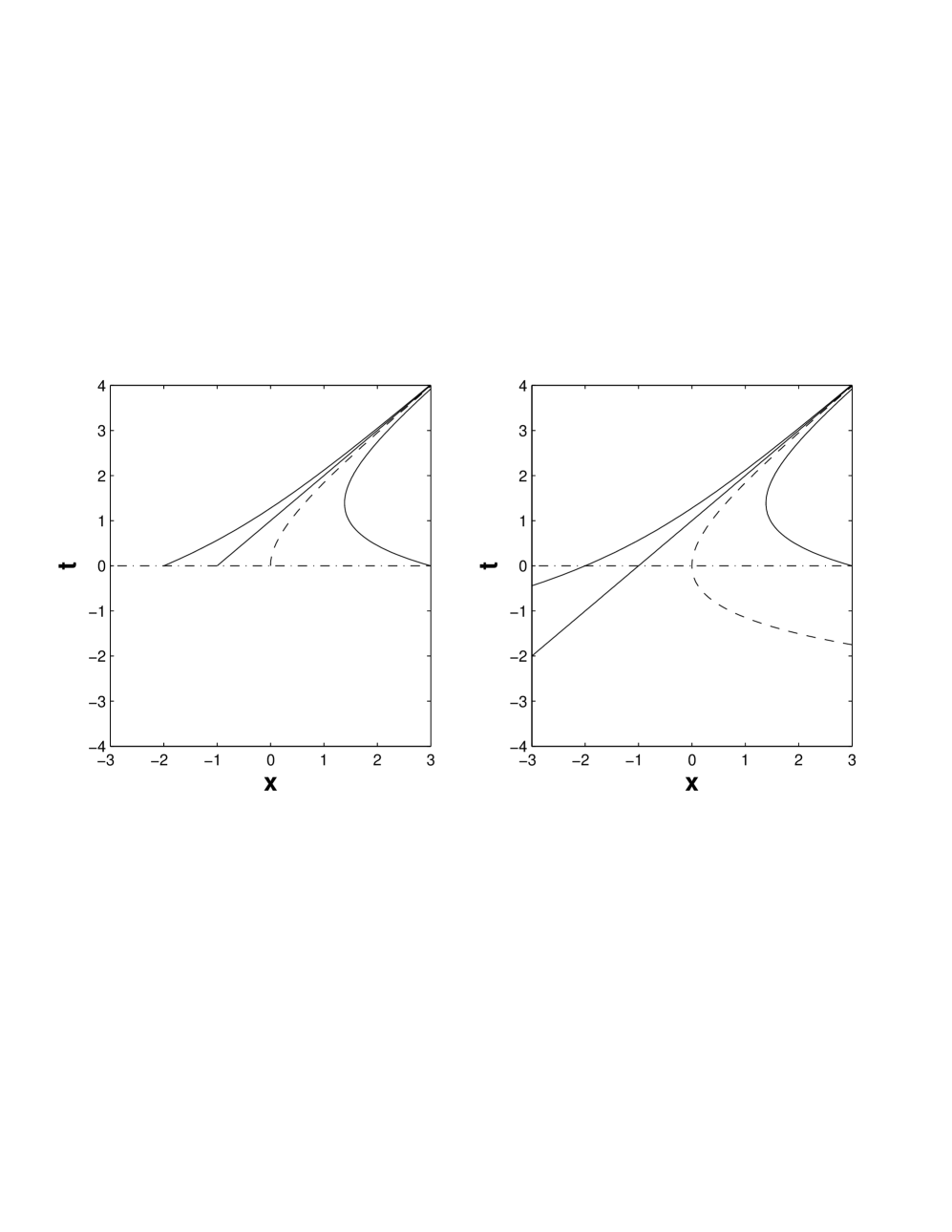
Figure 1a) displays several trajectories starting at times ranging from $t=0$ to $t=4$ and figure 1b) displays the same but starting at time $t=-4$ (note that in this case part of the trajectories are out of the displayed domain). For each initial condition the function $M$ provides the length of the projection of the trajectory over the $x$-axis in the range of times $[-\tau,\tau]$. Geometrically it is clear that in this example the function $M$ should have a minimum for a certain $x$ value and that this value depends on $\tau$. Ideally the minimum of $M$ should coincide with the position of the DHT at $t=0$, however this would not be possible if in the definition of $M$ only positive times were considered, i.e. if the limits of the integration were $(0,\tau)$ the dashed trajectory in figure 1a) would have a lower projection in positive times than the particular solution. An analogous problem would be encountered were only negative times considered, that is if the limits of the integration would have been $(-\tau,0)$. To determine precisely the position of the DHT at $t=0$, both positive and negative times must be considered in the definition of $M$. Figure 1b) confirms that with this choice the dashed trajectory cannot be distinguished, as it increases its projection in negative times. Figure 2a) displays the function $M(x^{*})_{t=0,\tau}$ evaluated along the trajectories (6), for several $\tau$ values. Figure 2b) displays the position of the minimum of the function $M_{t=0,\tau}$ as a function of $\tau$. These minima correspond to the positions of the $\tau$-distinguished trajectories at $t=0$ and as $\tau$ increases they approximate the coordinate of the DHT at this time, which is at $x^{*}=-1$. The pair $(t^{l},{\bf x}^{l})$ formed by the time at which $M$ is computed and the value of the coordinate ${\bf x}^{l}$ to which the minimum of the function $M_{t^{l},\tau}$ converges for increasing $\tau$ is called the limit coordinates. The graphic 2b) illustrates the idea of approaching a point $(t_{0},{\bf x}_{0})$ of the distinguished trajectory by means of the limit coordinates. In practice the convergence to the limit coordinates cannot be examined in the limit $\tau\to\infty$, either because it is impracticable in a numerical implementation, or because in the large $\tau$ limit errors accumulate, or simply because the dynamical system is defined by a finite time data set. For these reasons the convergence to the limit coordinates will be tested up to a finite $\tau$.

Figure 2b) raises the question: what controls the rate of the convergence of the minima of $M$ to the coordinates of the DHT? It is hard to answer this question rigorously for a vector field as general as in Eq. (2). However, some insight may be provided by particular examples. For instance the system

$$\frac{dx}{dt} = -2x+2t-1,$$ (7)

has the same DHT as (5). Its solution through the point $x^{*}$ at $t=0$ is given by

$$x(t)=t-1+e^{-2t}(x^{*}+1).$$ (8)

Here the decay of the solution towards the DHT is faster due to the presence of the exponential term $e^{-2t}$. Figure 3 shows that in this case the rate of the convergence of the minima of $M$ towards the coordinates of the DHT at time $t=0$ is also faster than before. However there exist systems in which the exponential decay of the solution is not a determining factor affecting the rate of the convergence of the minima of $M$ to the coordinates of the DHT. For instance, in autonomous systems fixed points are the DTs, and clearly they are minimizers of $M$ for any $\tau>0$ whatever is the exponential rate of growth or decay of the nearby solution.

In these examples the function $M$ has a unique minimum, but as we will see the situation will not always be so simple when nonlinearities are involved in the vector field. Also it is important to notice that the function $M$ obtained at different $\tau$ values has been used to obtain the limit coordinates $(t^{l}_{0},{\bf x}^{l}_{0})$ and that these approach the ${\bf x}_{0}$ coordinate of DHT at a given time $t_{0}$ (here $t_{0}=t_{0}^{l})$. Once this is obtained, approaching the DHT at later times $t_{k}=t_{0}+k\Delta t$ would require applying the same procedure to get the limit coordinates $(t^{l}_{k},{\bf x}^{l}_{k})$. We remark here that the proposed algorithm does not ensure that the set of limit coordinates $(t^{l}_{k},{\bf x}^{l}_{k})$ are in fact part of a trajectory. Later we will see that in practice, in many examples these points approach a true trajectory, however in realistic aperiodic flows this has to be verified a posteriori. These considerations lead us to the definition of a Distinguished Trajectory.

Definition 3

(Distinguished trajectory). A trajectory $\gamma(t)$ is said to be Distinguished with accuracy $\epsilon$ ($\,0\leq\epsilon$ ) in a time interval $[t_{0},t_{N}]$ if there exists a continuous path of limit coordinates $(t^{l},{\bf x}^{l})$ where $t^{l}\in[t_{0},t_{N}]$, such that,

$$||\gamma(t^{l})-{\bf x}^{l}(t^{l})||\leq\epsilon,\,\,\forall t^{l}\in[t_{0},t_{N}].$$ (9)

Here $||\cdot||$ represents the distance defined by

$$||{\bf a}-{\bf b}||=\sqrt{\sum_{i=1}^{n}(a_{i}-b_{i})^{2}}\,\,\,\,\,{with}\,\,\,\,{\bf a},{\bf b}\in\mathbb{R}^{n}.$$

In the numerical exploration of this definition we will replace the continuous path of limit coordinates $(t^{l},{\bf x}^{l})$ and the continuous trajectory $\gamma(t)$ by discrete representations $(t^{l}_{k},{\bf x}^{l}_{k})$ and $\gamma(t^{l}_{k})$ where $t_{0}\leq t^{l}_{k}\leq t_{N}$. By definition 3 any trajectory is distinguished for sufficiently large $\epsilon$, however the interesting distinguished trajectories are those for which $\epsilon$ is close to zero, which means it is of the order of the accuracy in which $\gamma(t^{l}_{k})$ and ${\bf x}^{l}(t^{l}_{k})$ are numerically determined, or zero, if an exact expression is known for both.

Underlying definitions 2 and 3 is the geometrical idea that distinguished trajectories, which act as organising centres of the flow in phase space, are those that ”move less” (in a certain sense) than other nearby trajectories. This property of “moving less” is satisfied by minima of the function $M$ as it measures the length of the displacement in phase space of a trajectory forwards and backwards in time. In fact this property is related somehow to property (2) of the definition provided in [17] and presented at the beginning of Section 2, as the trajectory that “moves least” is not expected to leave the neighbourhood $\mathcal{B}$.

Definitions 2 and 3 are made for a general dynamical system in any dimension $n$. The purpose of this paper is the exploration of these definitions, but more in an illustrative than demonstrative way, as it is impossible to provide examples for every possible $n$, and one cannot deal with every possible example at a given $n$. Even if one wants to provide a rigorous formal proof that the definition recovers specific trajectories such as periodic orbits (it is not obvious that in general they have to satisfy our definition), this has to be done with some further hypotheses on the vector field and proofs will not be valid beyond the assumed hypotheses. Therefore we restrict the discussion to dimensions up to 3, as these are the dimensions important for geophysical flows, which are what originally motivated the definition. However it is sensible to make the same definition for any dimension $n$, as it is clear that it works for autonomous systems of any dimension. Fixed points are the kind of trajectory expected to be recovered by the definition and they do not move at all in the phase space. For these $M=0$, while $M>0$ for any other trajectory in the neighbourhood which is not a fixed point.

We conclude this section with some remarks. First, it is not guaranteed a priori that for an arbitrary vector field, satisfying only some rather general hypotheses such as those of Eq. (2), the function $M$ will have a minimum, however this is not a problem from the point of view of the definition. For instance the same thing happens for general non-linear autonomous systems. In these systems fixed points are perfectly defined although one does not know a priori if such points exist for arbitrary examples. If they exist, it is possible to find them by either solving the nonlinear equation ${\bf v}({\bf x})=0$, or by applying definitions 2 and 3. In the same way one does not know a priori if distinguished trajectories exist for a general vector field however if they exist they can been found with the tools proposed in this article. Second, even if a path of limit coordinates is found it is not guaranteed that it will be a trajectory, although if that is the case then from definition 3 follows that this trajectory is distinguished. Third, one might think that if limit coordinates are found at $t_{0}$ that approach with great accuracy a point of an existing DT, then the iterative procedure described above for finding a set of limit coordinates $(t^{l}_{k},{\bf x}^{l}_{k})$ approaching the DT at later times is an unnecessary computational effort, as those coordinates could have been equally well obtained by integrating forwards the initial data. However there exist examples such as a hyperbolic DT in dimension greater than one with at least 1D unstable manifold, that cannot be integrated like this, as the integrated trajectory will eventually leave the neighbourhood of the DT through the unstable manifold no matter how small the initial error is. In summary the proposed methodology based on limit coordinates provides a systematic way of finding DT, which can be elusive and difficult to obtain. We will discuss these issues in detail in later sections.

3 A numerical algorithm

In this section we propose an algorithm for computing a path of limit coordinates in a time interval, and we verify that it is close to a DT of a known example. For this purpose we calculate, at increasing $\tau$ values, the minimum of the function $M_{t=0,\tau}({\bf x})$ for ${\bf x}$ in an open set in $\mathbb{R}^{n}$. The method is illustrated in a 2D case, the periodically forced Duffing equation

$$\dot{x} = y,$$

$$\dot{y} = x-x^{3}+\varepsilon\sin(t),$$ (10)

where $\varepsilon$ is a small parameter. The hyperbolic fixed point of the unperturbed autonomous system (i.e., $\varepsilon=0$) is at the origin ${\bf x}=(0,0)$. For small $\varepsilon$, it is possible to compute by perturbation theory (see [23]), the following periodic trajectory which stays close to the origin:

$${\bf x}_{DHT}(t)=-\frac{\varepsilon}{2}\binom{\sin t}{\cos t}-\frac{\varepsilon^{3}}{40}\binom{2\sin^{3}t+\frac{3}{2}\sin t\cos^{2}t}{\frac{3}{2}\cos^{3}t+3\sin^{2}t\cos t}+\mathcal{O}(\varepsilon^{5}).$$ (11)

For $\varepsilon=0.1$, Eq. (11) is accurate up to the fifth digit. This trajectory is identified as Distinguished in Ref. [17], for this reason we have labelled it a $DHT$. Substituting the expression,

$${\bf x}=(x,y)={\bf x}_{DHT}(t)+\left(\xi_{1},\xi_{2}\right)$$ (12)

into Eq. (10) and by dropping the nonlinear terms one finds that the linearized equations have two linearly independent solutions in terms of which the time evolution of the components ${(\xi_{1},\xi_{2})}$ is:

$$\left(\xi_{1},\xi_{2}\right)=\alpha\,{e}^{t}\left(\begin{array}[]{c}1/\sqrt{2}\\ 1/\sqrt{2}\end{array}\right)+\beta\,{e}^{-t}\left(\begin{array}[]{r}-1/\sqrt{2}\\ 1/\sqrt{2}\end{array}\right)+\mathcal{O}(\varepsilon^{2}).$$ (13)

Eq. (13) confirms the hyperbolicity of the solution (11).

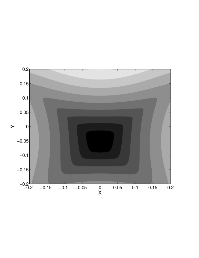
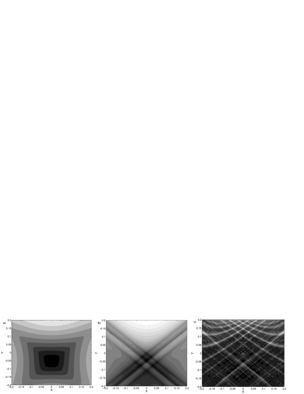
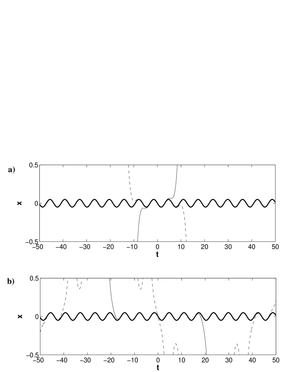
This explicit expression for the distinguished hyperbolic trajectory is a benchmark for testing the utility of our definition. The procedure starts by determining the coordinates of ${\bf x}_{DHT}$ at time $t=0$. We consider the open set ${\mathcal{D}}\subset\mathbb{R}^{2}$, defined by ${\mathcal{D}}=(-0.2,0.2)\times(-0.2,0.2)$ and in the function $M_{t=0,\tau}({\bf x})$ we take $\tau$ to be $2$. Figure 4 displays a contour plot of $M_{t=0,\tau=2}({\bf x})$ which has a minimum at ${\bf x}=(0,-5.7057\cdot 10^{-2})$. $M_{t=0,\tau=2}({\bf x})$ quantifies displacements of particles in phase space, and its minimum corresponds to the initial condition that “moves less” over the $\tau$ interval $[-2,2]$. As noted in the previous section, when the value of $\tau$ is increased, the position of the minimum gets closer and closer to the coordinates of the DHT at $t=0$. Figure 5 shows contour plots of the function $M$ for several $\tau$ values. Fig. 5a) displays a typical hyperbolic structure for $M$ for $\tau=5$ where the directions of the stable and unstable manifolds are easily recognised. In Fig. 5a) the function $M$ has a unique minimum at ${\bf x}=(0,-4.979\cdot 10^{-2})$ while in Fig. 5b) there appear several minima for $\tau=10$. The global minimum in this picture corresponds to ${\bf x}=(0,-5.0042565261\cdot 10^{-2})$. Figure 6a) compares the $x$-coordinate of ${\bf x}_{DHT}$ as a function of time with trajectories having initial conditions at the global minima of $M_{t=0,\tau=2}$ and $M_{t=0,\tau=10}$. Taking as initial condition the global minimum of $M_{t=0,\tau}$ for $\tau=10$ provides a trajectory that stays close to ${\bf x}_{DHT}$ for a longer time interval than for $\tau=2$, which confirms that larger $\tau$-values more closely approach the coordinates of the DHT. Fig. 5c) displays the contour plot of $M_{t=0,\tau=50}({\bf x})$. Its global minimum is at ${\bf x}=(0,-5.0037606418\cdot 10^{-2})$. The associated trajectory depicted in Fig. 6b) shows that this initial condition tracks the DHT for a longer time interval than those obtained for $\tau=2$ and 10, however the figure shows that the integration of the DHT in $(-50,50)$ is not possible. In fact the associated trajectory stays close to the DHT only in the time interval $(-20,20)$. This confirms that results obtained for $\tau=50$ are the same as those obtained for $\tau=20$. In practice for a finite precision numerical scheme, such as a 5th order Runge Kutta used here, the approach to the DHT has an upper bound depending on $\tau$. This occurs because the stable and unstable manifolds of the hyperbolic trajectory magnify any initial error in either negative or positive time and beyond this $\tau$-limit numerical errors dominate. The convergence towards the DHT is confirmed in Fig. 7 which displays the evolution of the coordinates $x$ and $y$ of the global minimum of $M$ as a function of the parameter $\tau$.

New minima appearing in Figs. 5b) and c) relate to the existence of different $\tau$-distinguished trajectories. As illustrated in Fig. 6b), they correspond to trajectories which stay close to ${\bf x}_{DHT}$ in a small time range contained in the interval $-\tau<t<\tau$, but which later fly apart from the DHT.

We now describe a numerical scheme to compute a path of limit coordinates. The algorithm has the following steps:

1. Step 1. Discretize the domain ${\mathcal{D}}$ at the initial time $t=t_{0}$ at which one wishes to compute a DT. For instance, the grid size of this domain in Fig. 4 is $101\times 101$. The function $M$ is evaluated at each grid point for a given $\tau_{0}$.

2. Step 2. Search for the local minima of $M_{t_{0},\tau_{0}}$ in the interior of the grid. These minima approach the coordinates of $\tau_{0}$-distinguished trajectories within the accuracy of the grid. In what follows we restrict our description to the case of a unique minimum, as this simplifies the description; the procedure is easily generalised to the case of multiple minima.

3. Step 3. Improve the approach of the coordinates of the $\tau_{0}$-distinguished trajectory up to precision $\delta$. For this purpose build up a $3^{n}$ grid centred on the candidate point provided by step 2, (for the 2D case this is a $3\times 3$ grid as Fig. 8 illustrates), setting the distance between nodes equal to $\delta$. Then evaluate $M_{t_{0},\tau_{0}}$ at the points of the $\delta$-grid. If the minimum of $M_{t_{0},\tau_{0}}$ is in the interior of the grid, then the coordinates of the $\tau_{0}$-distinguished trajectory are known to within $\delta$ accuracy. Otherwise the $\delta$-grid must be rebuilt centred on the boundary point where the minimum has been located, and $M_{t_{0},\tau_{0}}$ must be re-evaluated in the new $\delta$-grid. This procedure stops when the minimum of $M_{t_{0},\tau_{0}}$ is in the interior of the grid.

4. Step 4. Computing the limit coordinates at time $t_{0}$. Define a sequence of increasing $\tau$-values as follows: $\tau_{1}=\tau_{0}+\Delta\tau$ and $\tau_{2}=\tau_{0}+2\Delta\tau$. Then evaluate $M_{t_{0},\tau_{0}}$, $M_{t_{0},\tau_{1}}$ and $M_{t_{0},\tau_{2}}$ on the $\delta$-grid. If the minimum is at an interior position for the three cases, then we consider that limit coordinates have been found within $\delta$ accuracy. We note that this is a necessary but not sufficient condition as one does not know a priori the convergence rate to the distinguished trajectory. Although this criterion could be strengthened, it has been tested and found to be adequated for the examples explained in subsequent sections. If the condition defined above of having a minimum at an interior position for the sequence of $\tau$-values is not satisfied then, after replacing $\tau_{0}$ by $\tau_{1}$, we return to step 3 and then to step 4. The loop between steps 3 and 4 is stopped when the condition of step 4 is satisfied for some $\tau_{k}$.

5. Step 5. Compute the limit coordinates at time $t_{1}=t_{0}+\Delta t$. Once the limit coordinates have been approached at time $t_{0}$, they are integrated forward numerically up to time $t_{1}$. If the limit coordinates converge to a hyperbolic DT with an unstable manifold, the position ${\bf x}(t_{1})$ obtained should deviate from the position of the DT at time $t_{1}$. In order to correct this, the procedure described above is repeated from step 3 onwards. For that purpose in the definition of $M$, $t_{0}$ is replaced by $t_{1}$ and the $\tau$-value is reset to $\tau_{0}$. The coordinates ${\bf x}(t_{1})$ are the first approximation to the $\tau_{0}$-distinguished trajectory at time $t_{1}$. Once the limit coordinates are found for time $t_{1}$ it is possible to repeat the procedure to locate them at successive times $t_{2},t_{3},\ldots,t_{N}$.

The algorithm requires as inputs: an explicit expression for the dynamical system (2); the definition of the domain $\mathcal{D}\subset\mathbb{R}^{n}$; the initial and final times $t_{0}$, $t_{N}$ at which DTs are required, and the time step $\Delta t$ for intermediate times; the initial $\tau_{0}$ and the increment $\Delta\tau$; the precision $\delta$. As an output the algorithm gives a path of limit coordinates at the selected times $t_{k}$.

Next we discuss in more detail some technical aspects related to the implementation of the above algorithm. Steps 1 and 3 require evaluating $M_{t_{0},\tau_{0}}$ as defined in Eq. (3). We explain how this is done for the contour plots displayed in Figs. 4 and 5, which refer to the system (10) at $t_{0}=0$. Fig. 9 shows a schematic projection onto the $\mathbb{R}^{2}$ plane of a possible trajectory ${\bf x}(t)$ of the system from $-\tau$ to $\tau$. As it was obtained numerically, only a finite number of points ($L$) appear. This picture suggests the following discrete version of Eq. (3) for $M$:

$$M({\bf x})_{0,\tau}=\sum_{j=1}^{L-1}\left(\int^{p_{f}}_{p_{i}}\!\!\!\sqrt{\left(\frac{dx_{j}(p)}{dp}\right)^{2}+\left(\frac{dy_{j}(p)}{dp}\right)^{2}}dp\right),$$ (14)

where the functions $x_{j}(p)$ and $y_{j}(p)$ represent a curve interpolation parametrized by $p$, and the integral

$$\int^{p_{f}}_{p_{i}}\!\!\!\sqrt{\left(\frac{dx_{j}(p)}{dp}\right)^{2}+\left(\frac{dy_{j}(p)}{dp}\right)^{2}}dp$$ (15)

is computed numerically. In our case we use the Romberges method (see [25]) of order $2K$ with $K=5$. It is clear that the accuracy of the evaluation of $M$ will depend on the number of points on the trajectory $L$, which is controlled by the size of the time step, $h$, of the integrator (a 5th order Runge Kutta method) and on the interpolation scheme between points. Two interpolation methods are compared in tables (1) and (2). Results in table (1) are obtained with linear interpolation between nodes. Results in table (2) correspond to the interpolation method used by Dritschel [26] in the context of contour dynamics, which has been successfully applied in [23] to the computation of invariant manifolds for aperiodic flows. This method interpolates a piece of the curve in Fig. 9 between consecutive nodes as follows:

$${\bf x}_{j}(p)={\bf x}_{j}+p{\bf t}_{j}+\eta_{j}(p){\bf n}_{j}$$ (16)

for $p_{i}=0\leq p\leq p_{f}=1$ with ${\bf x}_{j}(0)={\bf x}_{j}$ and ${\bf x}_{j}(1)={\bf x}_{j+1}$, where:

$${\bf t}_{j} = (a_{j},b_{j})={\bf x}_{j+1}-{\bf x}_{j},\,\,\,{\bf t}_{j}\in\mathbb{R}^{2}$$ (17)

$${\bf n}_{j} = (-b_{j},a_{j}),\,\,\,{\bf n}_{j}\in\mathbb{R}^{2}$$ (18)

$$\eta_{j}(p) = \mu_{j}p+\beta_{j}p^{2}+\gamma_{j}p^{3},\,\,\,\eta_{j}\in\mathbb{R}.$$ (19)

The cubic interpolation coefficients $\mu_{j}$, $\beta_{j}$ and $\gamma_{j}$ are

$$\mu_{j}=-\frac{1}{3}d_{j}\kappa_{j}-\frac{1}{6}d_{j}\kappa_{j+1},\,\,\,\beta_{j}=2d_{j}\kappa_{j},\,\,\,\gamma_{j}=\frac{1}{6}d_{j}(\kappa_{j+1}-\kappa_{j}),$$

where $d_{j}=|{\bf x}_{j+1}-{\bf x}_{j}|$ and

$$\kappa_{j}=2\frac{a_{j-1}b_{j}-b_{j-1}a_{j}}{|d^{2}_{j-1}{\bf t}_{j}+d^{2}_{j}{\bf t}_{j}-1|}$$

is the local curvature defined by the circle through the three points, $x_{j-1}$, $x_{j}$, and $x_{j+1}$.

Tables (1) and (2) show the errors in the computed lengths of the ellipses for different ratios of major to minor axis. The reference length is that obtained with GNU Octave version 2.1.73, as it provides 16 correct digits for the known circumference. The tables confirm that the Dritschel’s method is superior to linear interpolation and it is the one used to compute the function $M$. In the trajectory from $-\tau$ to $\tau$ the number of points $L$ is determined by the time step size of the Runge Kutta method which is set to $10^{-2}$.

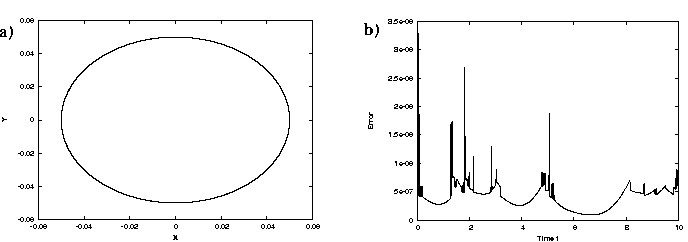
Another important element of the algorithm needing discussion is the value of the input parameters, in particular of $\tau_{0}$ and $\Delta\tau$. It is clear from Fig. 5 that large $\tau$ values are not convenient as they increase the roughness of the function $M$ and several local minima may appear in the neighbourhood of a DHT that correspond to trajectories that stay close to it for some time. On the other hand it is clear that sufficiently large $\tau$ values are required to fix the coordinates of the DHT to within prescribed accuracy. Combining these observations suggests the use of relatively small values for the initial $\tau_{0}$. In the example above $\tau_{0}=2$, provides, as a starting point, a smooth $M$ as that of Fig. 4. The increments should not be large. In practice we have chosen $\Delta\tau=\tau_{0}/2$. This prevents from stepping to a too rough $M$ before getting close enough to the sought after DHT. Some of the local minima appearing in Fig. 5b) are just apparent and disappear with a more refined grid. However, as already observed, others belong to true $\tau$-distinguished trajectories, which are secondary and can be avoided if the increment of the $\tau$-values is conveniently small. These choices are found to be appropriate for determining with great accuracy the DHT in (11) by means of a path of limit coordinates. Figure 10a) represents both the analytical DHT and the numerical limit coordinates and Figure 10b) displays the distance between the exact and the numerical approach, confirming that the DHT in (11) is also a DT in the sense of our definition 3 with accuracy $\epsilon=10^{-6}$. Other parameters in the algorithm are: $\delta=10^{-6}$, step size in the Runge Kutta method $h=10^{-2}$, $t_{0}=0$, $t_{N}=6$, and $\Delta t=0.01$. To locate the DHT with accuracy $\delta=10^{-6}$ requires increasing values of $\tau$ up to 15, which is near the limit of the integration method. Figure 11 shows the maximum $\tau$ required at each $t_{k}$.

4 Applications to exact examples

In this section we apply the algorithm explained in the previous section to selected examples.

4.1 A non-hyperbolic distinguished trajectory

The unperturbed autonomous system (10) obtained with $\varepsilon=0$ has non-hyperbolic fixed points at $(-1,0)$ and $(1,0)$. Obviously these fixed points correspond to DTs which are also $\tau$-distinguished trajectories for all $\tau>0$. For the periodically forced system (10) with small $\varepsilon$ it is possible using perturbation theory to find periodic solutions close to these fixed points in a manner similar to the analysis of the hyperbolic example made in the previous section. For instance close to the point $(1,0)$ we find the periodic trajectory:

$$x_{DET}(t)=-\binom{1}{0}+\varepsilon\binom{\sin t}{\cos t}+3\varepsilon^{2}\binom{\frac{1}{2}\cos^{2}t}{-\sin t\cos t}+\mathcal{O}(\varepsilon^{3}).$$ (20)

This solution has not been considered Distinguished in previous works [17, 18], as these have been focused on hyperbolic trajectories and this solution, as is proved next, is not hyperbolic. However, in anticipation of its having the Distinguished property, we have labelled it $DET$ for two reasons. One is that it is periodic, and we expect periodic orbits to be distinguished, and second is that it is in clear correspondence to the elliptic fixed point (-1,0) in the case $\varepsilon=0$, and fixed points are DTs.

To determine the stability of (20) we proceed as before, by substituting the expression

$${\bf x}=(x,y)={\bf x}_{DET}(t)+\left(\xi_{1},\xi_{2}\right)$$ (21)

into Eq. (10). We find that the linearized system at order $\varepsilon^{0}$ is:

$$\frac{d\xi_{1}}{dt} = \xi_{2}$$ (22)

$$\frac{d\xi_{2}}{dt} = -2\xi_{1}.$$ (23)

Therefore the linearized flow around ${\bf x}_{DET}(t)$ evolves according to:

$$\left(\xi_{1},\xi_{2}\right)=\alpha\,{e}^{i\sqrt{2}t}\left(\begin{array}[]{c}1/\sqrt{3}\\ i\sqrt{2/3}\end{array}\right)+\alpha^{*}\,{e}^{-i\sqrt{2}t}\left(\begin{array}[]{r}1/\sqrt{3}\\ -i\sqrt{2/3}\end{array}\right)+\mathcal{O}(\varepsilon),$$ (24)

which clearly is not hyperbolic. Here $\alpha$ and $\alpha^{*}$ are complex conjugate numbers.

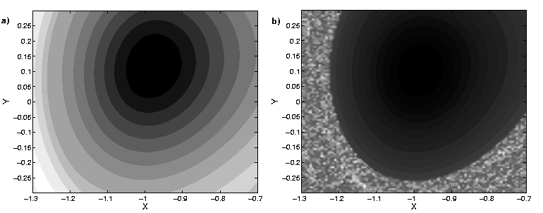
We apply our algorithm to determine the limit coordinates approaching (20), as we want to verify whether definition 3 also works for time-dependent non-hyperbolic solutions. The following input is considered: ${\mathcal{D}}=(-1.2,-0.8)\times(-0.2,0.2)$, $\tau_{0}=2$, $\Delta\tau=1$, $\delta=10^{-4}$, $t_{0}=0$, $t_{N}=6$, and time step $10^{-2}$ for the Runge-Kutta integrator. We note that the accuracy $\delta$ is not as demanding as before, since now the exact ${\bf x}_{DET}$ for $\varepsilon=0.1$ is only accurate up to the third digit. Figure 12 shows a rather different structure for the function $M$. An important feature is the smoothness of $M$ close to the DET even for large $\tau$. In figure 12b) the differences between the rather flat region around the position of the DT given by (20), which appears in the dark tone, and the roughness of the outer part are remarkable. The irregularity of this region suggests that inside it nearby trajectories follow rather different paths as happens for chaotic motions, while the regularity of the central core suggests the existence of trapped trajectories circling around the DET. From this perspective the function $M$ for large $\tau$ seems a useful tool for fixing the boundaries of a Lagrangian eddy, different to the methods proposed in [27, 29].

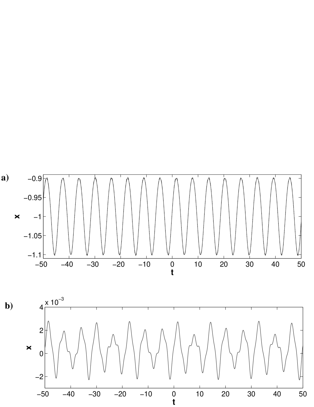
Figure 13 shows the rate of convergence to the global minimum of $M$ in the domain ${\mathcal{D}}$ as a function of $\tau$. The convergence towards the coordinates of the DT is oscillatory and rather slow since $\tau$ values up to $600$ are required. A slight difference between the exact coordinates of the DT and the numerically computed limit coordinates is evident, however we note that these differences are consistent with the precision to which the exact DT is known, which is only to the third digit. Figure 14, and more specifically figure 14b), confirms that the exact expression in Eq. (20) is in fact a distinguished trajectory according to our definition 3 with accuracy $\epsilon=4\cdot 10^{-3}$.

Figure 15a) shows a forward and backward integration along the time interval $(-50,50)$ taking as initial data the limit coordinates supplied by our algorithm at time $t_{0}=0$, and compares it with the exact solution of the DT. From figure 15b) it can be seen that this trajectory evolves close to the exact solution in the entire time range. This result shows that contrary to what happens near hyperbolic trajectories, near non hyperbolic trajectories, small error does not amplify and as consequence, once a DT is known to exist it could have been computed simply by integrating forwards and backwards the limit coordinates found at a given time $t_{k}$. However one needs to be careful here, as a trajectory is not necessarily distinguished at all times, and for it to be properly called distinguished, it should be verified that it stays close to the limit coordinates in the whole time interval, and therefore one cannot avoid computing limit coordinates along the time interval in this case either. We will return to this point in the next section.

4.2 The rotating Duffing equation

Next we analyse the aperiodic hyperbolic distinguished trajectory of a system already studied in [23], the rotating Duffing equation:

$$\left(\begin{array}[]{c}\dot{\eta_{1}}\\ \dot{\eta_{2}}\end{array}\right) = \left(\begin{array}[]{cc}\sin 2\omega t&\cos 2\omega t+\omega\\ \cos 2\omega t-\omega&-\sin 2\omega t\end{array}\right)\left(\begin{array}[]{c}\eta_{1}\\ \eta_{2}\end{array}\right)$$ (31)

$$+ (\varepsilon\sin t-[\cos\omega t\eta_{1}-\sin\omega t\eta_{2}]^{3})\left(\begin{array}[]{c}\sin\omega t\\ \cos\omega t\end{array}\right).$$ (34)

This Duffing equation is quasi-periodic in time when the rotation rate $\omega$ is irrational. It is obtained from the system (10) by applying the rotation ${\bf x}=R(t)\boldsymbol{\eta}$, where

$$R(t)=\left(\begin{array}[]{cc}\cos\omega t&-\sin\omega t\\ \sin\omega t&\cos\omega t\end{array}\right).$$ (37)

The DHT can also be obtained through the coordinate transformation:

$${\boldsymbol{\eta}}_{DHT}(t)=R(t)^{-1}{\bf x}_{DHT}(t).$$ (38)

Figure 16, and in particular Fig. 16b), confirms that the DHT (38) is also a DHT according to our definition  3 with accuracy $\epsilon=4\cdot 10^{-6}$.

4.3 A 3D extension of the Duffing equation

In this section we apply our definitions to an example in higher dimension. In particular we consider a 3D extension of the Duffing equation:

$$\dot{x} = y,$$

$$\dot{y} = x-x^{3}+\varepsilon\sin(t),$$ (39)

$$\dot{z} = z+\varepsilon\sin(t).$$

The hyperbolic fixed point of the unperturbed autonomous system (i.e., $\varepsilon=0$) is at the origin ${\bf x}=(0,0,0)$. The solution for small $\varepsilon$ becomes:

$${\bf x}_{DHT}(t) = -\frac{\varepsilon}{2}\left(\begin{array}[]{c}\sin t\\ \cos t\\ {\small\cos t-\sin t}\end{array}\right)$$ (43)

$$- \frac{\varepsilon^{3}}{40}\left(\begin{array}[]{c}{2\sin^{3}t+\frac{3}{2}\sin t\cos^{2}t}\\ {\frac{3}{2}\cos^{3}t+3\sin^{2}t\cos t}\\ 0\end{array}\right)+\mathcal{O}(\varepsilon^{5}).$$ (47)

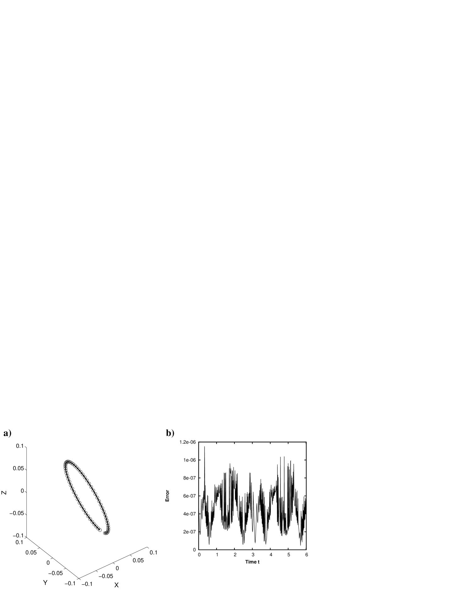
The numerical scheme explained in Section 3 is easily adapted to higher dimensions. However some changes must be made. The computation of $M$ requires approximating lengths of trajectories which in 3D needs an interpolation scheme different to that of Eq. (16), which is only valid in $\mathbb{R}^{2}$. We consider the linear interpolation instead. This interpolation evaluates the function $M$ satisfactorily if trajectories are represented by a large number of points. This is achieved by using a Runge-Kutta method with time step $h=10^{-4}$. Figure 17 indicates the evolution of coordinates associated with the minimum of $M$ as a function of $\tau$ (solid line). The dashed line corresponds to the exact perturbative solution. There is evident a clear convergence towards the exact position although there is a significant jump in the asymptotic behaviour beyond $\tau\sim 50$. This jump is due to round off errors in the determination of $M$ for large $\tau$. The third equation in (39) is just a linear equation and for this reason solutions which are in the neighbourhood of the DHT have $z$-coordinate growing exponentially in backwards time. Thus for large $\tau$ values, the evaluation of $M$ is made along very long trajectories in the $z$-coordinate, which are underrepresented by points sampled every $h=10^{-4}$ (see table I) and where lengths are badly calculated by adding up very small and very large (and inaccurate) numbers. In spite of this, figure 18 confirms that the exact distinguished trajectory can be accurately obtained with our methodology and that for $\tau<50$ errors are within the expected margin. The remaining input parameters used in Figs. 17 and 18 are: ${\mathcal{D}}=(-0.2,0.2)\times(-0.2,0.2)\times(-0.2,0.2)$, $\tau_{0}=2$, $\Delta\tau=1$, $\delta=10^{-6}$, step size $h=10^{-4}$ in the Runge Kutta method, $t_{0}=0$, $t_{N}=6$, and $\Delta t=10^{-2}$.

As we explain next, the computational demands made by this example are considerably larger than they were for the previously considered 2D examples. When determining a DT, most of the CPU time is spent computing the value of $M$ on the $\delta$-grid displayed in Fig. 8. The number of neighbours of the interior point grows with the dimension $n$ as $3^{n}$, therefore when the problem increases its dimension from $n$ to $n+1$, the computational demands are multiplied by 3. Another factor that contributes to increased computational time is the decrease of the Runge Kutta time step $h$ in the evaluation of trajectories on the $\delta$-grid. This increases the number of points in the trajectory (and therefore the number of operations) with respect to the previous Dristchel approach by a factor $100$. This factor is partially balanced by the fact that for the same number of points the arclength is computed more rapidly with the linear than with the Dristchel interpolation.

5 Application to vector fields defined as finite time data sets

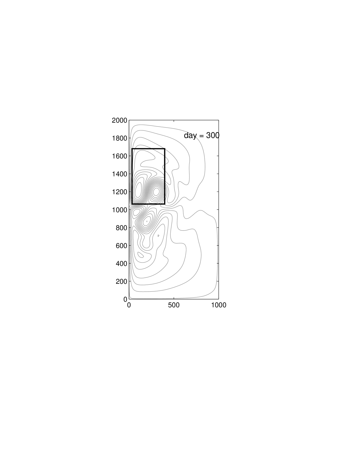
In this section we explore definition 3 for a highly aperiodic 2D flow in which the vector field is defined as a finite time data set. In particular we consider the output of a quasigeostrophic wind-driven double gyre model in a regime already studied in [11, 12]. Details of this model may be found in [12, 21]. Fig. 19 shows a typical output for the streamfunction provided by this model. The velocity data set is obtained on a 1000 km $\times$ 2000 km rectangular domain and spans 4000 days. This interval is considered for a fluid started from rest and allowed to spin for 25000 days. Free slip conditions are considered for the velocities on the boundaries and the wind stress curl is 0.32 dyn/cm². The equations of motion for this system are given by:

$$\dot{x} = v_{x}(x,y,t)=-\frac{\partial\psi}{\partial y},$$ (48)

$$\dot{y} = v_{y}(x,y,t)=\frac{\partial\psi}{\partial x},$$ (49)

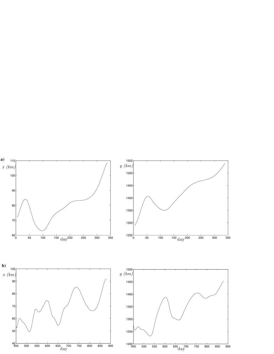
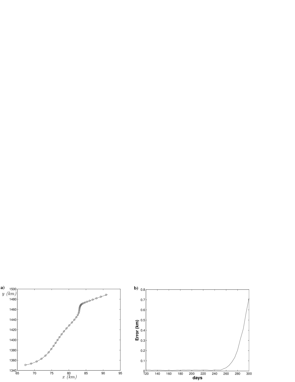
and the variables $x$ and $y$ are in the rescaled domain $[0,1]\times[0,2]$. Here the velocity fields $v_{x}$ and $v_{y}$ are provided as a finite time data set and are interpolated using bicubic interpolation in space and 3rd order Lagrange polynomials in time. This method has been reported to be good enough for integrating trajectories in [24]. We will focus our analysis in the time interval $[0,900]$ in the area marked by a rectangle in Fig. 19 for which [12] reports the computations of several DHTs. In [12] distinguished trajectories are computed by means of an iterative algorithm which is initialized on a hyperbolic instantaneous stagnation point (ISP). In particular two paths of such ISPs are chosen in the Northern gyre in the time intervals $[0,339]$ and $[446,880]$. From each of these paths, a DHT is computed which is in the same geographical area although its coordinates are determined for a different time range. In Fig. 20 we show the $x$ and $y$ evolutions for these trajectories. These coordinates have been computed with a different algorithm to that proposed in [12]. Instead each corresponds to a trajectory which is in the intersection of a piece of a stable manifold and a piece of an unstable manifold which are evolved in backwards and forwards time respectively. In this procedure, in order to avoid the numerous intersections between stable and unstable manifolds, which make difficult the tracking of the trajectory which is distinguished, manifolds are trimmed at each time step following the ideas in [11] where a method is described to compute a piece of single branch of the stable or of the unstable manifold. This method takes advantage of the fact that a DHT must be in the intersection of both manifolds at all times, as it is a trajectory, however does not improve the method explained in [12] in the sense that it does not allow either to extend the computation of the DHT beyond the time interval in which the ISP exists. Many questions have been raised for these trajectories as has been discussed in [11, 12]. For instance as they have been computed only in finite time intervals on which the ISP exists, one can ask how to pursue its computation beyond that interval. Another open issue in [12] concerns deciding if the two DHT in Fig. 20 computed at different times are part of the same trajectory. In [11], the question is raised of whether it can happen that a DHT ceases to be distinguished or hyperbolic. In this section we apply our algorithm to compute limit coordinates and verify whether trajectories in Fig. 20 are distinguished or not following our definition 3. Also we will describe how this definition helps address the questions raised in [11, 12]. We have applied our algorithm to compute limit coordinates in the domain in which the DHT shown in Fig. 20a) exists. In particular we have applied it with the input: $\mathcal{D}=(55,75)\times(1325,1375)$ km², $t_{0}=120$, $t_{N}=300$, $\Delta t=5$ days, $\tau_{0}=2$ days, $\Delta\tau=5$ days, and $\delta=10^{-3}$ km. The time step of the Runge-Kutta method is $0.1$ days. Fig. 21a) indicates with a solid line the projection onto the $x-y$ plane of the trajectory depicted in figure 20a) in the interval $(120,300)$, and with circles the path of limit coordinates. Fig. 21b) shows the evolution of the distances between these trajectories. This confirms that the trajectory displayed in Fig. 20a) is also distinguished in the sense of definition 3 in the time interval $[120,330]$ with accuracy $\epsilon=8\cdot 10^{-1}$ km. Thus in this time interval, limit coordinates give a method for computing DT different from those proposed in [12, 17]. Circles in Fig. 22 show the location versus time of the $x$ limit coordinates computed with our algorithm. The solid line represents a trajectory obtained after integrating with a 5th order Runge-Kutta method forwards and backwards in time the initial condition of the circle at day 285. The dashed line represents the same, but with the initial condition slightly perturbed. It is evident that in both cases the trajectories are aligned with the path of limit coordinates. The distinguished trajectory is highly hyperbolic backwards in time as in that direction a small perturbation amplifies greatly, while it does not do so forwards in time, suggesting that it has a non-hyperbolic type of stability in that direction (see comments to Figs. 6 and 15).

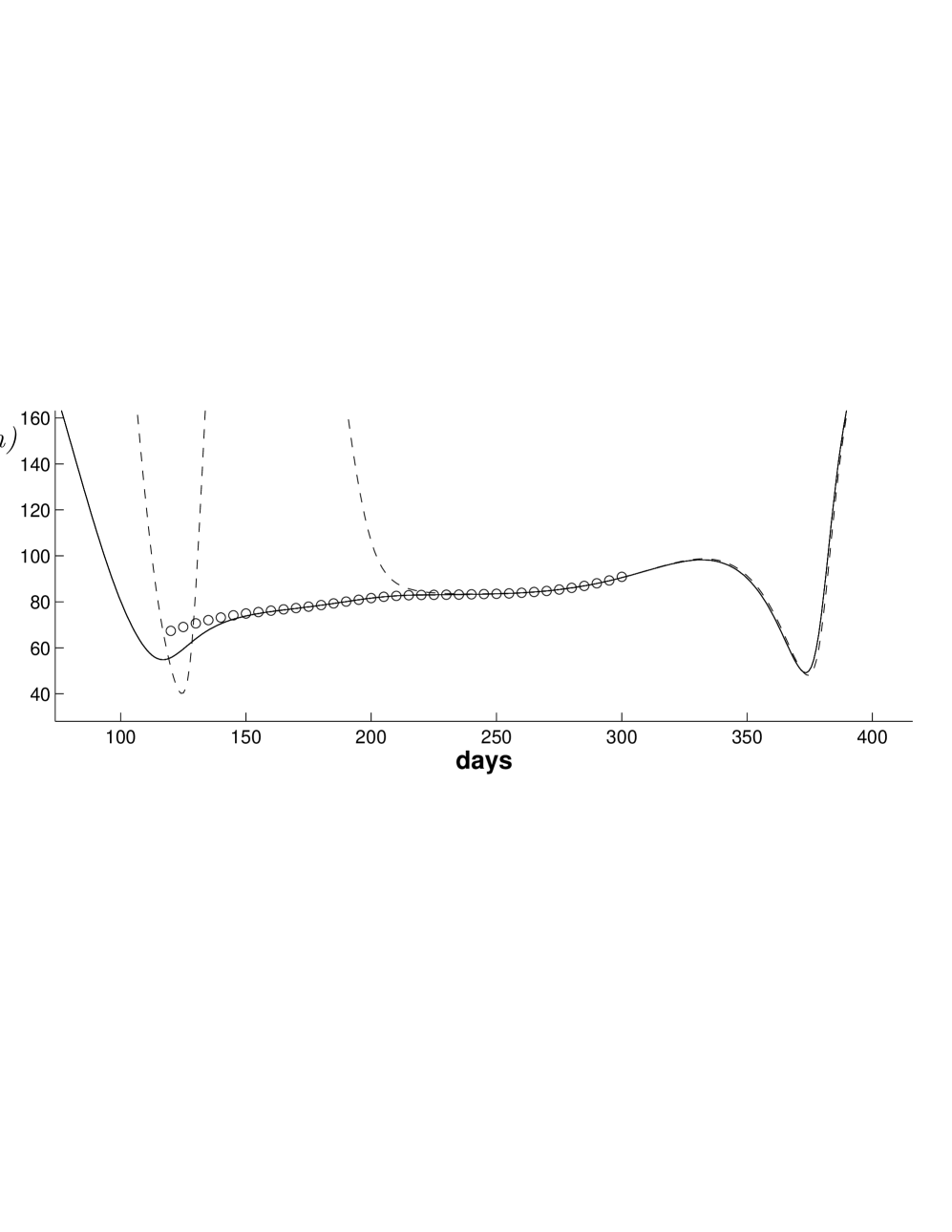
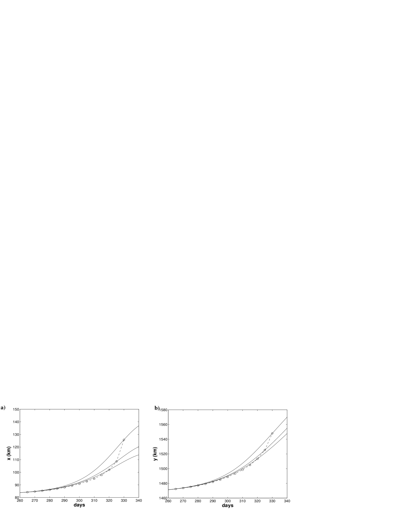
Beyond day 300 it is possible to continue the path of limit coordinates. Figure 23 shows a diagram at day 330; there is shown the convergence of the $x$ component of the minimum of $M$ versus $\tau$. This type of convergent diagram is not found in this neighbourhood for day 337. On the other hand, although it is possible to continue the path of limit coordinates beyond day 300, Fig. 24 proves that this path is not a trajectory. There can be seen the existence of different trajectories crossing the path, confirming that it is not a trajectory as otherwise it would violate the uniqueness of the solution. Therefore, following our construction it is possible to say that beyond day 300 the trajectory is no longer distinguished.

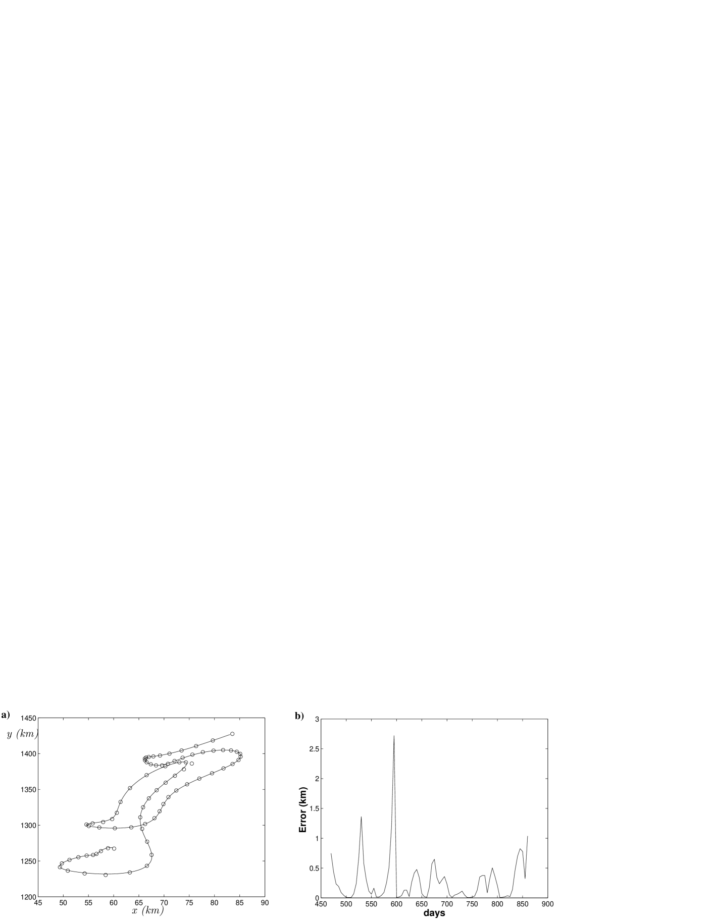
Fig. 25 confirms that the trajectory in Fig. 20b) is also distinguished in the sense of definition 3 in the time interval $(470,860)$ with accuracy $\epsilon=3$ km. In particular to compute the path in Fig. 25 we have applied the algorithm of section 3 with the input: $\mathcal{D}=(50,65)\times(1255,1270)$ km², $t_{0}=470$, $t_{N}=860$, $\Delta t=5$ days, $\tau_{0}=2$ days, $\Delta\tau=7$ days, and $\delta=10^{-3}$ km. The Runge-Kutta time step is $0.1$ days. In the time interval from day 600 to day 650 some of the input parameters were modified as follows: $\mathcal{D}=(73.5,75.5)\times(1384,1392)$ km², $\tau_{0}=40$ days, and $\Delta t=1$ day. This was due to the presence of nearby elliptic type minima in the function $M$, that made difficult tracking the path of the limit coordinates with the previous input.

Finally, we discuss the existence of non-hyperbolic distinguished trajectories in this data set. The presence of this type of trajectories has not been addressed before, and we do not have any benchmark solution. We have looked for this type of trajectory in areas of the flow where Eulerian eddies seemed to persist for long times. Figure 26 represents the function $M$ at day 370 for $\tau=150$ and $\tau=250$. In these figures there can be seen the structure of an eddie at the centre even for rather long $\tau$-values, however figure 27 does not confirm the convergence of the minimum of $M$ towards a constant value. On the other hand, the slow convergence in diagram 13 towards the non-hyperbolic trajectory, already suggested that long time intervals were required for that purpose, and those intervals might be difficult to find in realistic flows such like the one analysed here, in which one is provided just with a finite time datat set.

6 Conclusions

In this paper we have proposed a new definition of distinguished trajectory that attempts to extend the concept of fixed point and periodic orbit to aperiodic dynamical systems. The concept of fixed point is trivially contained in the definition. Regarding other especially useful trajectories in dynamical systems, for instance periodic orbits, we have not proved that they fall within the definition in a general way, but we have numerically verified it for selected 2D and 3D examples. The definition can be implemented numerically and the procedure consists in determining a path of limit coordinates. We have analysed exact examples for the Duffing equation with known distinguished trajectories, both periodic an aperiodic, and we have found that the path of limit coordinates coincides, to within numerical accuracy, with the distinguished trajectories and therefore those trajectories are identified also as distinguished in the framework of our definition. Our definition is novel with respect to previous works dealing with distinguished trajectories, because it is applicable to non-hyperbolic trajectories. In particular we have studied a periodic orbit of the Duffing equation with non-hyperbolic stability and is also recognised as distinguished by our definition. In this case the function $M$ from which the limit coordinates are computed seems to be a suggestive tool for characterising Lagrangian eddies. We have tested our definition in the context of realistic aperiodic flows where distinguished hyperbolic trajectories had been found [11, 12]. Again we have identified these trajectories by paths of limit coordinates in certain time intervals. Beyond these time intervals the trajectories are no longer distinguished according to our definition. Thus in the context of the definitions provided in this paper, the property of a trajectory of being distinguished may be lost in time. Also we have found evidence that the hyperbolicity of these trajectories is not constant in time. These two statements provide answers to the open questions mentioned in the text that have been addressed in [11, 12].

Figure captions

Figure 1

Solutions (6) for different initial conditions $x^{*}$. a) Solutions for positive times $t>0$. b) Solutions for positive and negative times.

Figure 2

a) Function $M(x^{*})_{t=0,\tau}$ evaluated over the solutions (6). Dashed line $\tau=3$, solid line $\tau=4$. b) Position of the $x^{*}$-coordinate at the minimum of the function $M_{t=0,\tau}$ as a function of $\tau$. The horizontal dashed line marks the position of the DHT.

Figure 3

Position of the $x^{*}$-coordinate at the minimum of the function $M_{t=0,\tau}$ as a function of $\tau$. The function $M_{t=0,\tau}$ is considered for the solutions in (8). The horizontal dashed line marks the position of the DHT.

Figure 4

Contour plot of the function $M_{t=0,\tau=2}({\bf x})$ in the open set ${\mathcal{D}}=(-0.2,0.2)\times(-0.2,0.2)$. The minimum corresponds to the black tone.

Figure 5

Contour plot of the function $M$ in the open set ${\bf x}\in(-0.2,0.2)\times(-0.2,0.2)$. a) $M_{t=0,\tau=5}({\bf x})$; b) $M_{t=0,\tau=10}({\bf x})$; c) $M_{t=0,\tau=50}({\bf x})$.

Figure 6

a) $x$-coordinate versus time for the DHT (thick solid line) and those trajectories integrated with initial conditions at the global minima of Figs. 5a) (solid line) and b) (dashed line); b) $x$-coordinate versus time for the DHT (thick solid line), a trajectory integrated with initial condition at the global minimum of Fig. 5c) (solid line) and a trajectory integrated at a non-global but relative minimum of the same figure (dashed line).

Figure 7

Evolution of the coordinates of the global minimum of $M$ versus $\tau$. a) The $x$ coordinate; b) the $y$ coordinate. These plots show the convergence to the DHT whose position is marked with a dashed horizontal line.

Figure 8

A $\delta$-grid in $\mathbb{R}^{2}$. The centre or interior point is marked with the white dot.

Figure 9

A schematic projection onto the $\mathbb{R}^{2}$ plane of a possible trajectory from $-\tau$ to $\tau$ with $L$ points.

Figure 10

a) Representation of both the distinguished hyperbolic trajectory (11) and its approximation obtained with the proposed numerical algorithm for $\varepsilon=0.1$; b) distance between the exact and the numerical approach.

Figure 11

Representation of the maximum $\tau$ required to approach the DT to within accuracy $\delta=10^{-6}$ versus time.

Figure 12

Contour plot of the function $M$ in the open set ${\bf x}\in(-1.2,-0.8)\times(-0.2,0.2)]$. a) $M_{t=0,\tau=10}({\bf x})$; b) $M_{t=0,\tau=300}({\bf x})$.

Figure 13

Evolution of the coordinates of the global minimum of $M$ versus $\tau$ at $t_{0}=0$. a) The $x$ coordinate; b) the $y$ coordinate. These plots show the convergence of the minima to the coordinates of the DET whose position is marked with a continuous horizontal line.

Figure 14

a) Dotted line represents the exact non-hyperbolic distinguished trajectory and the solid line stands for the numerically computed limit coordinates; b) distance between the exact non-hyperbolic trajectory (20) and the limit coordinates.

Figure 15

a) $x$-coordinate versus time for the DET (solid line) and the trajectory integrated taking as initial data the limit coordinates located at time $t_{0}=0$ (dashed line); b) time evolution of the differences between these trajectories.

Figure 16

a) Dashed line represents the exact distinguished hyperbolic trajectory of the rotating Duffing equation and the solid line stands for the numerically computed one; b) distance between the exact and the numerical distinguished hyperbolic trajectories.

Figure 17

Evolution of the coordinates of the global minimum of $M$ for the 3D example versus $\tau$ at $t_{0}=0$. a) The $x$ coordinate; b) the $y$ coordinate; c) the $z$ coordinate. These plots show the convergence of the minima to the coordinates of the DHT whose position is marked with a dashed horizontal line.

Figure 18

a) The solid line represents the exact distinguished hyperbolic trajectory of the 3D equation and circles stand for numerically computed coordinates; b) distance between the exact and the numerical distinguished hyperbolic trajectories.

Figure 19

Contour plot of the streamfunction produced by the quasigeostrophic model at day 300.

Figure 20

Distinguished hyperbolic trajectories in the Northern gyre of the quasigeostrophic model reported in [12]. a) Evolution of the $x$ and $y$ coordinates in the time interval $[5,338]$; b) evolution of the $x$ and $y$ coordinates in the time interval $[450,880]$

Figure 21

a) Solid line represents the projection on the phase space of the distinguished hyperbolic trajectory depicted in Fig. 20a) and circles stands for the numerically computed limit coordinates; b) distance between the trajectories represented in a).

Figure 22

Circles stand for the $x$ component of the limit coordinates in the time range where they approach a DT. The solid line represents a trajectory integrated with a 5th order Runge-Kutta method passing the through limit coordinates at day 285. The dashed line is a trajectory integrated from the same condition plus a small perturbation.

Figure 23

a) $x$ component of the minimum of $M$ versus $\tau$ at day 330; b) $y$ component of the minimum of $M$ versus $\tau$ at the same day.

Figure 24

a) Circles stand for the $x$ component of the limit coordinates versus time and the solid lines stand for different trajectories; b) the same as a) but for the $y$ component.

Figure 25

a) Solid line represents the projection on the phase space of the distinguished hyperbolic trajectory depicted in Fig. 20b) and circles stands for the numerically computed limit coordinates; b) distance between the trajectories represented in a).

Figure 26

a) Contour plot of $M_{t=370,\tau=150}$, the elliptic minimum is in the dark area almost at the centre; b) contour plot of $M_{t=370,\tau=250}$.

Figure 27

a) $x$ component of the minimum of $M$ versus $\tau$ at day 370; b) $y$ component of the minimum of $M$ versus $\tau$ at the same day.

Table captions

Table 1

Relative errors for several ellipse lengths, computed with a linear interpolation over $L$ points on the curve.

Table 2

Relative errors for several ellipse lengths, computed with Dritschel interpolation over $L$ points on the curve.

	Linear interpolation
$L$	Ratio between axes
	$1$	$2$	$5$	$10$	$100$	$1000$
$10$	$8.16$	$8.80$	$9.48$	$9.73$	$9.99$	$10.00$
$10^{2}$	$2.63$	$3.36$	$3.86$	$3.99$	$4.05$	$4.05$
$10^{3}$	$0.83$	$1.08$	$1.24$	$1.29$	$1.31$	$1.31$
$10^{4}$	$0.26$	$0.34$	$0.39$	$0.41$	$0.41$	$0.41$
$10^{5}$	$8.34\times 10^{-2}$	$0.11$	$0.12$	$0.13$	$0.13$	$0.13$
$10^{6}$	$2.64\times 10^{-2}$	$3.42\times 10^{-2}$	$3.94\times 10^{-2}$	$4.08\times 10^{-2}$	$4.14\times 10^{-2}$	$4.14\times 10^{-2}$
$10^{7}$	$8.34\times 10^{-3}$	$1.08\times 10^{-2}$	$1.25\times 10^{-2}$	$1.29\times 10^{-2}$	$1.31\times 10^{-2}$	$1.31\times 10^{-2}$
$10^{8}$	$2.64\times 10^{-3}$	$3.42\times 10^{-3}$	$3.95\times 10^{-3}$	$4.08\times 10^{-3}$	$4.14\times 10^{-3}$	$4.14\times 10^{-3}$
$10^{9}$	$8.34\times 10^{-4}$	$1.08\times 10^{-3}$	$1.25\times 10^{-3}$	$1.29\times 10^{-3}$	$1.31\times 10^{-3}$	$1.31\times 10^{-3}$

Table 1:

	Dritschel interpolation
$L$	Ratio between axes
	$1$	$2$	$5$	$10$	$100$	$1000$
$10$	$0.99$	$0.67$	$0.33$	$0.25$	$0.26$	$0.27$
$10^{2}$	$3.49\times 10^{-2}$	$1.37\times 10^{-2}$	$4.47\times 10^{-3}$	$2.81\times 10^{-3}$	$2.08\times 10^{-3}$	$2.61\times 10^{-3}$
$10^{3}$	$1.11\times 10^{-3}$	$3.83\times 10^{-4}$	$9.20\times 10^{-5}$	$4.43\times 10^{-5}$	$2.23\times 10^{-5}$	$1.98\times 10^{-5}$
$10^{4}$	$3.53\times 10^{-5}$	$1.17\times 10^{-5}$	$4.44\times 10^{-6}$	$5.23\times 10^{-6}$	$2.80\times 10^{-7}$	$7.01\times 10^{-7}$
$10^{5}$	$1.12\times 10^{-6}$	$3.64\times 10^{-7}$	$2.17\times 10^{-6}$	$4.48\times 10^{-6}$	$5.45\times 10^{-8}$	$9.20\times 10^{-7}$
$10^{6}$	$3.51\times 10^{-8}$	$1.14\times 10^{-8}$	$2.10\times 10^{-6}$	$4.46\times 10^{-6}$	$5.222\times 10^{-8}$	$9.22\times 10^{-7}$
$10^{7}$	$1.11\times 10^{-9}$	$3.68\times 10^{-10}$	$2.10\times 10^{-6}$	$4.46\times 10^{-6}$	$5.21\times 10^{-8}$	$9.22\times 10^{-7}$
$10^{8}$	$2.18\times 10^{-11}$	$1.30\times 10^{-11}$	$2.10\times 10^{-6}$	$4.46\times 10^{-6}$	$5.22\times 10^{-8}$	$9.22\times 10^{-7}$
$10^{9}$	$3.72\times 10^{-10}$	$3.37\times 10^{-10}$	$2.10\times 10^{-6}$	$4.46\times 10^{-6}$	$5.22\times 10^{-8}$	$9.25\times 10^{-7}$

Table 2:

Figure 1:

Figure 2:

Figure 3:

Figure 4:

Figure 5:

Figure 6:

Figure 7:

Figure 8:

Figure 9:

Figure 10:

Figure 11:

Figure 12:

Figure 13:

Figure 14:

Figure 15:

Figure 16:

Figure 17:

Figure 18:

Figure 19:

Figure 20:

Figure 21:

Figure 22:

Figure 23:

Figure 24:

Figure 25:

Figure 26:

Figure 27:

References

- [1] Aref, H., 1984. Stirring by chaotic advection. J. Fluid Mech. 143, 1 21.
- [2] Khakhar DV, Ottino J.M. Fluid mixing (stretching) by time-periodic sequences for weak flows. Physics of Fluids 29 11 3503-3505 (1986).
- [3] Dombre T., Frisch U., Greene J.M., Henon M., Mehr A., Soward A.M. Chaotic Streamlines in the ABC flows Journal of Fluid Mechanics 167, 353-391 (1986).
- [4] Wiggins, S.: Chaotic Transport in Dynamical Systems, Springer- Verlag, New York, 1992
- [5] Wiggins, S.: Introduction to Applied Nonlinear Dynamical Systems and Chaos , Springer-Verlag, New York, 2003.
- [6] Guckenheimer, J., Holmes, P.: Nonlinear Oscillations, Dynamical Systems, and Bifurcations of Vector Fields, Springer- Verlag, New York, 2002
- [7] Malhotra, N. and Wiggins, S.: Geometric Structures, Lobe Dynamics, and Lagrangian Transport in Flows with Aperiodic Time Dependence, with Applications to Rossby Wave Flow, J. Nonlinear Sci., 8, 401 456, 1998.
- [8] Haller, G. and Poje, A.: Finite time transport in aperiodic flows, Physica D, 119, 3/4, 352 380, 1998.
- [9] Langa JA, Robinson JC, Suarez A. Stability, instability, and bifurcation phenomena in non-autonomous differential equations. Nonlinearity 15 (3) 887-903 (2002).
- [10] Langa JA, Robinson JC, Suarez A. Bifurcations in non-autonomous scalar equations. Journal of Differential Equations. 221 (1) 1-35 (2006).
- [11] Mancho A. M., Small D., Wiggins S., A tutorial on dynamical systems concepts applied to Lagrangian transport in oceanic flows defined as finite time data sets: Theoretical and computational issues. Physics Reports 437, 3-4 (2006).
- [12] Mancho, A. M., Small, D., Wiggins, S., 2004. Computation of hyperbolic and their stable and unstable manifolds for oceanographic flows represented as data sets. Nonlinear Process. Geophys. 11, 17 33.
- [13] Mancho A. M., Hernández-García E., Small D., Wiggins S., Fernández V. Lagrangian transport through an ocean front in the North-Western Mediterranean Sea. Journal of Physical Oceanography 38, 6, 1222-1237 (2008).
- [14] Aurell E., Boffetta G., Crisanti A., Paladin G., Vulpiani A. Predictability in the large: an extension of the concept of Lyapunov exponent. J. Phys. A: Math. General, 30: 1-26, 1997.
- [15] Haller, G. Distinguished Material surfaces and coherent structures in three-dimensional fluid flows. Physica D, 149: 248-277, 2001.
- [16] Nese JM, Quantifying local predictability in phase space. Physica D 35: 237-250, 1989.
- [17] Ide, K., Small, D., Wiggins, S., 2002. Distinguished hyperbolic trajectories in time dependent fluid flows: analytical and computational approach for velocity fields defined as data sets. Nonlinear Process. Geophys. 9, 237 263.
- [18] Ju, N., Small, D., Wiggins, S., 2003. Existence and computation of hyperbolic trajectories of aperiodically time-dependent vector fields and their approximations. Int. J. Bif. Chaos 13, 1449 1457.
- [19] G. Haller. Exact theory of unsteady separation for two dimensional flows. Journal of Fluid Mechanics 512, 257-311 (2004)
- [20] Eisenbach S., Friedrich R., Large-eddy simulation of flow separation on an airfoil at a high angle of attack and Re=10(5) using Cartesian grids. Theoretical and Computational Fluid Dynamics 22 (3-4) 213-225 (2008).
- [21] Coulliette, C., Wiggins, S., 2001. Intergyre transport in a wind-driven, quasigeostrophic double gyre: an application of lobe dynamics. Nonlinear Process. Geophys. 8, 69 94.
- [22] Szeri, A., Leal, L. G., and Wiggins, S.: On the Dynamics of Suspended Microstructure in Unsteady, Spatially Inhomogeneous Two-Dimensional Fluid Flows, J. Fluid Mech., 228, 207 241, 1991.
- [23] Mancho, A. M., Small, D., Wiggins, S., Ide, K.,2003. Computation of Stable and Unstable Manifolds of Hyperbolic Trajectories in Two-Dimensional, Aperiodically Time-Dependent Vectors Fields. Physica D 182, 188-222.
- [24] Mancho, A. M., Small, D., Wiggins, S., Ide, K.,2006. A comparison of methods for interpolating chaotic flows from discrete velocity data. Computers and Fluids 35, 416-428.
- [25] W.H. Press, S.A. Teukolsky, W.T. Vetterling, B.P. Flannery, Numerical Recipes in Fortran 77, The Art of Scientific Computing, 2nd ed., Cambridge University Press, Cambridge, 1999.
- [26] Dritschel, D.G., Contour dynamics and contour surgery: numerical algorithms for extended, high-resolution modelling of vortex dynamics in two-dimensional, inviscid, incompressible flows, Comput. Phys. Rep. 10 (1989) 77 146.
- [27] Branicki, M, Mancho, A. M., Wiggins, S. A Lagrangian description of transport associated with a Front-Eddy interaction: application to data from the North-Western Mediterranean Sea. Preprint submitted for publication.
- [28] D. B. Chelton, M. G. Schlax, R. M. Samelson, and R. A. de Szoeke, Global observations of large oceanic eddies, Geophysical Research Letters 34 (2007), L15606.
- [29] Haller G, An objective definition of a vortex, Journal of Fluid Mechanics 525, 1-26 (2005).