Self-consistent theory of molecular switching

Abstract

We study the model of a molecular switch comprised of a molecule with a soft vibrational degree of freedom coupled to metallic leads. In the presence of strong electron-ion interaction, different charge states of the molecule correspond to substantially different ionic configurations, which can lead to very slow switching between energetically close configurations (Franck-Condon blockade). Application of transport voltage, however, can drive the molecule far out of thermal equilibrium and thus dramatically accelerate the switching. The tunneling electrons play the role of a heat bath with an effective temperature dependent on the applied transport voltage. Including the transport-induced “heating” selfconsistently, we determine the stationary current-voltage characteristics of the device, and the switching dynamics for symmetric and asymmetric devices. We also study the effects of an extra dissipative environment and demonstrate that it can lead to enhanced non-linearities in the transport properties of the device and dramatically suppress the switching dynamics.

I introduction

The apparent limitations of the silicon-based technology on the way to further acceleration and miniaturization have prompted active research into alternative electronic architectures.molecular ; hybrid_Likharev In particular, molecular electronics holds a lot of promise because each molecule, being only about a nanometer in size can in principle perform such non-trivial operations as information storagemem or electrical current rectification.mol_diod Since molecules, even intricate ones, can be mass produced by means of well-controlled chemical synthesis, one expects them to be less susceptible to the issues of disorder that plague the silicon-based electronics below the 10 nm scale. The ultra-miniaturization that molecular electronics affords, however, also leads to the problem of connecting the molecular elements among each other, as well as of the necessary interfacing with large-scale conventional electronics. Indeed, early on, this problem has caused many difficulties in reproducing results from one device to another.nature However, recent advances in fabricationrecent_expt as well as better theoretical understanding of physics and chemistry at the point of contact recent_th demonstrate that this difficulty is not fundamental and promise to make reliable and reproducible molecular junctions a reality.

There is, however, a fundamental difference that distinguishes the molecular devices from the conventional semiconductor ones. For a molecule to perform its unique function, it has to be well isolated from most environmental influences, except for the (metallic or semiconducting) contacts that are required to access it. Under standard operation of the device, the chemical potentials differ by the value of the applied transport voltage $V$ mutiplied by the electron charge $e$, and thus the environment that the molecule experiences can not be considered as equilibrium if the voltage is greater than the temperature, $eV>k_{B}T$ ($k_{B}$ being Boltzmann constant). Therefore, to determine the behavior of a molecular device under such conditions, one needs to determine selfconsistently the influence, e.g. of electrical current on the molecular dynamics, and vice versa, the influence of non-thermal vibrations or electronic excitations of the molecule on the current. This is very different from the conventional electronics where devices are rarely driven out of thermal equilibrium far enough to significantly affect the performance (exceptions are the non-linear devices, such as Gunn diod).

One of the most promising and interesting molecular devices is a switch, which can be used for information storage. Switching has been observed experimentally in several molecular junctions.sw_expt Proposed theoretical explanations for switching range from (a) large and small-scale molecular conformational changes, (b) changes in the charge state of the molecule, or (c) combination of the two, or “polaronic”. The purely electronic switching mechanism (b), while possible, appears quite impractical since it would require a separate contact in order to change the charge state of the part of the molecule that would play the role analogous to the floating gate in flash memory by electrostatically affecting the “channel” current. The switching mechanisms (a) and (c) upon closer inspection turn out to be fundamentally the same, since in order to be able to switch and read out the conformational state of the molecule electronically there necessarily has to be a coupling between the electronic and ionic degrees of freedom. The dynamical stability of the “on” and “off” states in these mechanisms is achieved due to the collective nature of the states, which now involve not only the electronic occupancy but also all the positions of the ions in the molecule. Thus the change of the charge state of the molecules is accompanied by the ionic rearrangement, which for strong enough electron-ion coupling can dramatically slow down the charge state switching. This is the essence of the Franck-Condon “blockade.” braig ; vonOppen ; MHM ; galperin By chemically engineering molecules with strong electron-ion coupling and soft (low frequency) vibrational modes one can achieve arbitrarily slow equilibrium switching rates.

In order for molecular memory element to be useful, it has to have a long retention time (slow switching rate in the absence of any drive) but fast write time, i.e. it should be possible to accelerate the switching rate by gate or transport voltages. It is easy to see that in molecular switches with polaronic mechanism the transport-driven switching acceleration occurs naturally. As soon as the transport voltage exceeds the vibrational energy quantum, $eV>\hbar\omega_{0}$, additional transport, as well as switching, channels open, which correspond to electron tunneling on and off the molecule with simultaneous excitation of vibrational quanta.MHM ; vonOppen Moreover, enhanced charge fluctuations on the molecule effectively “heat up” the molecule, further increasing the current through the device. This leads to a positive feed-back loop which saturates when the energy transferred to the molecule from non-equilibrium tunneling electrons exactly balances the energy transferred back from the molecule to electrons. As a result, the stationary switching rate can vastly exceed the equilibrium switching strongly suppressed due to the Franck-Condon physics.

Most of the molecular devices studied experimentally so far have been weakly coupled to the leads.park ; yu ; park2 ; zhit ; qiu ; chae ; cnt This corresponds to the bare tunnel broadening $\hbar\Gamma$ of molecular electronic levels smaller that the energy required to excite one oscillator quantum (phonon) $\hbar\omega_{0}$. The single-electron effects play a crucial role in this case. They are well theoretically described by a model of a single-electron tunneling (SET) device coupled to a single-mode harmonic oscillator, developed mostly in the context of nanoelectromechanical systems. In the strong-coupling regime, when the electron-ion interaction energy $E_{p}$ (defined below) exceeds $\hbar\omega_{0}$, the physics is governed by the Franck-Condon effect, i.e. when the tunneling of an electron onto the molecule with the simultaneous emission or absorption of several phonons is more probable than elastic tunneling. The current as the function of voltage exhibits steps separated by $\hbar\omega_{0}/e$, schoeller ; braig ; mitra ; aji and the non-equilibrium electronic heating of the molecular vibrational mode leads to self-similar avalanche dynamics of current with the intervals of large current alternating with the periods of strongly suppressed current.vonOppen

In this paper, we study the case of “slow” phonons at strong coupling, $\Gamma\gg\omega_{0}$ for $eV>\hbar\omega_{0}$.galperin ; MHM ; armour ; doiron ; fabio The physical distinction between this case and the one of “fast” phonons, $\Gamma\ll\omega_{0}$, can be understood in the following way. For fast phonons, every electron tunneling event occurs over many oscillator periods. Thus effectively electrons can only couple to (or “measure”) the energy (i.e. occupation number) of the oscillator.zurek ; MarZur In the opposite regime, $\Gamma\ll\omega_{0}$, electron tunneling is fast, and thus electrons are sensitive to the position of the oscillator. Therefore, in the former case, as a result of electron tunneling, the oscillator density matrix becomes close to diagonal in occupation number basis (and thus non-classical), and in the latter case, it is nearly diagonal in the position basis (and thus classical). In Ref. MHM, it has been rigorously demonstrated for arbitrary coupling that the condition for the onset of the classical (Langevin) dynamics is given by $\min(\hbar\Gamma,eV)\gg\hbar\omega_{0}$. Even at weak coupling, $E_{p}<\hbar\omega_{0}$, if a high enough bias is applied between the leads, the oscillator dynamics becomes non-trivial, with the possibility of switching between stationary states of different amplitudes. blanter At strong couplings, $E_{p}>\hbar\omega_{0}$, there is another kind of multistability that appears at relatively small voltages, $eV<E_{p}$ – the system can switch between the states corresponding to (approximately) 1 and 0 electrons on the molecule. This multistability and switching can be described within the generalization of the Born-Oppenhemier approach to open systems.MHM In the metallic case the appearance of the multistability and the current suppression as a function of the bias voltage is associated with a discontinuity of the current (when the cotunnelling is neglected).fabio

The slow (or “classical”) phonon strong coupling case is attractive since besides switching between the different charge-ion states, it allows a read-out of the state by means of cotunneling transport through the molecule. In cotunneling, the charge state of the molecule changes only virtually for a period of time determined by the energy uncertainty principle. This time can be much shorter than the vibration period, and thus the ionic configuration and the average charge occupancy need not change. On the other hand, in sequential tunneling, the tunneling events between the leads and the molecule are energy-conserving, with the rates determined by the Fermi’s Golden rule. Typically, cotunneling currents are much smaller than sequential ones since they are higher order in the tunneling matrix element. However, if the sequential tunneling is strongly suppressed by the Franck-Condon physics, the cotunneling, which needs not be affected by it, may dominate. In the case $\Gamma<\omega_{0}$ and strong electron-ion coupling the role of cotunneling was recently studied in Ref. andreev, , where it was found that while it does not destroy the Franck-Condon blockade, it can dramatically affect the low-voltage current and current noise, as well as the vibrational dynamics.

The purpose of this work is to provide a unified self-consistent description of the sequential and cotunneling transport regimes in the case of a molecular switch in the “classical” regime $\Gamma>\omega_{0}$ and $eV>\hbar\omega_{0}$. This regime allows for a systematic non-perturbative treatment for an arbitrary electron-ion coupling strength.MHM We determine the dynamics of the vibrational degree of freedom, the average current and current noise through the device, and the switching times as functions of transport and gate voltages. We also analyze the role of extrinsic dissipation.

II Model

We consider the model for a molecular switch proposed in Ref. MHM, ; galperin, . The molecule is modeled as a single electronic level $\hat{d}$ strongly interacting with a vibrational mode, $x$. It is located between two leads, from which electrons can tunnel into the electronic level. The interaction is provided by the force $\lambda$ (typically of electrostatic origin) acting on the molecule. The system is described by the Hamiltonian

$$H = (\epsilon_{0}+\lambda x)\hat{d}^{\dagger}\hat{d}+\frac{p^{2}}{2m}+\frac{m\omega_{0}^{2}x^{2}}{2}$$ (2)

$$+\sum_{k,\alpha}{\epsilon_{k\alpha}\hat{c}^{\dagger}_{k\alpha}\hat{c}_{k\alpha}}+\sum_{k,\alpha}{t_{\alpha}(\hat{c}^{\dagger}_{k\alpha}\hat{d}+\hat{d}^{\dagger}\hat{c}_{k\alpha})},$$

where $\alpha$ is the lead index ($L$ or $R$) and $\hat{c}$ and $\hat{d}$ are the electron annihilation operators for the leads and local orbital, respectively. We consider the model for spinless electrons for simplicity. (Inclusion of spin along with onsite Coulomb blockade should lead to qualitatively similar results.) The vibrational mode is characterized by the “bare” frequency $\omega_{0}$ and the effective mass $m$. The displacement and coordinates are described by the canonically conjugate operators $x$ and $p$. The coupling between the electronic level and the mode is characterized by the “polaron” energy $E_{p}=\lambda^{2}/(2m\omega_{0}^{2})$ and the coupling to the leads by tunnel rate $\Gamma_{\alpha}=\pi\nu_{\alpha}t_{\alpha}^{2}/\hbar$, where $\nu_{\alpha}$ is the density of states in lead $\alpha$. In Refs. MHM, ; galperin, it has been shown that for strong enough coupling, $E_{p}/\hbar\gg\Gamma_{L}+\Gamma_{R}$, the system can exhibit bi-stability, with one state corresponding to empty resonant level and non-displaced mode $x$, and the other to occupied level and the mode displaced by the amount $\sim\lambda/(m\omega_{0}^{2})$. In the previous work, Ref. MHM, , current and current noise were determined in the regime of small transport voltage, $|eV|\ll E_{p}$ (where $eV=\mu_{L}-\mu_{R}$) in the approximately “symmetric” situation, $\epsilon_{0}\approx E_{p}$. In the present work, we generalize the previous results for current and current noise as well as determine the behavior of the switching rates between the metastable states for arbitrary transport and gate voltages.

When electrons are driven out of equilibrium by an applied transport voltage, the dynamics of the vibrational mode becomes very simple, even for strong coupling between the mode and electrons. That is because when the characteristic timescale for electronic subsystem becomes shorter than oscillator frequency $\omega_{0}$, electrons appear to the mode as a “high-temperature,” albeit position dependent and strongly coupled bath. Physically, for any position $x$, the electronic bath adjusts (almost!) instantaneously, in a manner analogous to how electrons adjust to the instantaneous positions of ions in isolated molecules, as described by the Born-Oppenheimer approximation. Indeed, as in the standard Born-Oppenheimer approximation in equilibrium bulk solids, one effect of the non-equilibrium fast electronic environment is the modification of the effective potential experienced by the mode; however, what is more, the electronic subsystem, by virtue of being open, also provides force noise (fluctuations) and the dissipation to the mode. Since the force acting on the mechanical mode is simply $-\lambda n$, where $n=\hat{d}^{\dagger}\hat{d}$ is the occupation of the electronic mode, in order to obtain the average force and its fluctuation it is enough to calculate the average of $n$ and it’s fluctuation (charge noise) for a given static position $x$. When a weak time dependence of $x(t)$ is included one finds that a correction to the average of $n$ appears that is linear in $dx/dt$. This last term corresponds to the dissipation induced by the retardation of the electronic degrees of freedom, that do not respond immediately to a change of $x$ (first non-adiabatic correction).armour It can also be traced to the “quantum” nature of the charge noise, i.e. a slight asymmetry between the charge noise at positive and negative frequencies.aguado ; gardiner ; clerk As a result, the dynamics of the mode $x$ becomes essentially classical, described by the Langevin equation,MHM

$$m\ddot{x}+A(x)\dot{x}+m\omega_{0}^{2}x=F(x)+\xi(t),$$ (3)

where the position-dependent force $F$, damping $A$, and the intensity of the white noise $D$, $\langle\xi(t)\xi(t^{\prime})\rangle=D(x)\delta(t-t^{\prime})$ are related to the electronic Green functions on the Keldysh contour as

$$F(x) = -\frac{\lambda\hbar}{2\pi i}\int{d\omega G_{fr}(\omega,x)},$$ (4)

$$A(x) = \frac{\lambda^{2}\hbar}{2\pi}\int{d\omega G_{fr}(\omega,x)\partial_{\omega}G_{rf}(\omega,x)},$$ (5)

$$D(x) = \frac{\lambda^{2}\hbar}{2\pi}\int{d\omega G_{fr}(\omega,x)G_{rf}(\omega,x)}\ .$$ (6)

The zero temperature Green functions (for the forward-reverse Keldysh time path) are

$$G_{fr}(\omega,x) = 2i\frac{\hbar\Gamma_{L}\Theta(\mu_{L}-\hbar\omega)+\hbar\Gamma_{R}\Theta(\mu_{R}-\hbar\omega)}{(\hbar\omega-\epsilon_{0}-\lambda x)^{2}+\hbar^{2}\Gamma^{2}},$$ (7)

$$G_{rf}(\omega,x) = -2i\frac{\hbar\Gamma_{L}\Theta(\hbar\omega-\mu_{L})+\hbar\Gamma_{R}\Theta(\hbar\omega-\mu_{R})}{(\hbar\omega-\epsilon_{0}-\lambda x)^{2}+\hbar^{2}\Gamma^{2}}.$$ (8)

Here $\Gamma=\Gamma_{L}+\Gamma_{R}$. These expressions are valid also at finite but low temperatures such that $k_{B}T<\hbar\Gamma$. [At higher temperature the step functions $\Theta(\epsilon)$ have to be replaced by Fermi functions $n_{F}(-\epsilon/k_{B}T)$.] Therefore, at low temperatures, we obtain,

$$F(x) = -\frac{\lambda}{\pi\Gamma}\left[\Gamma_{L}\left(\tan^{-1}\frac{\mu_{L}-\epsilon-\lambda x}{\hbar\Gamma}+\frac{\pi}{2}\right)\right.$$ (9)

$$+\left.\Gamma_{R}\left(\tan^{-1}\frac{\mu_{R}-\epsilon-\lambda x}{\hbar\Gamma}+\frac{\pi}{2}\right)\right]\ ;$$

$$A(x) = \frac{\lambda^{2}\Gamma\hbar^{3}}{\pi}\left\{\frac{\Gamma_{L}}{[(\mu_{L}-\epsilon_{0}-\lambda x)^{2}+\hbar^{2}\Gamma^{2}]^{2}}\right.$$ (10)

$$+\left.\frac{\Gamma_{R}}{[(\mu_{R}-\epsilon_{0}-\lambda x)^{2}+\hbar^{2}\Gamma^{2}]^{2}}\right\}\ ;$$

$$D(x) = \frac{\lambda^{2}\Gamma_{L}\Gamma_{R}}{\pi\Gamma^{3}}\left(\tan^{-1}z+\frac{z}{z^{2}+1}\right)^{\frac{\mu_{L}-\epsilon_{0}-\lambda x}{\hbar\Gamma}}_{\frac{\mu_{R}-\epsilon_{0}-\lambda x}{\hbar\Gamma}}\ .$$ (11)

Note that the expression for the force is just $F=-\lambda n(x)$, where $n(x)$ is the occupancy of the $d$ level for a fixed displacement $x$. The expression for $D$ is given for $\mu_{L}>\mu_{R}$, otherwise, the $\mu_{L}$ and $\mu_{R}$ have to be interchanged.

III Current and Noise from the Fokker-Planck description

From the Langevin Eq. (3) one can derive a Fokker-Plank equation for the probability ${\cal P}(x,p,t)$ that at a given time $t$ the displacement and the momentum of the vibrational are $x$ and $p=m\dot{x}$,

$$\partial_{t}{\cal P}=-{p\over m}\partial_{x}{\cal P}-F(x)\partial_{p}{\cal P}+{A(x)\over m}\,\partial_{p}(p{\cal P})+{D(x)\over 2}\,\partial^{2}_{p}{\cal P}\,.$$ (12)

This Fokker-Plank equation can be used to study both the stationary properties of the system, as well as the time evolution from a given initial condition.

III.1 Current

Given our assumption about the separation between the slow ionic – vibrational – and fast electronic – tunneling – timescales, the problem of evaluating the stationary current reduced to the evaluation of the quasistationary current averaged over the fast electronic times for a fixed position $x$ and momentum $p$ of the mode, with the consequent averaging over the stationary probability distribution, ${\cal P}(x,p)$. In our case, the quasistationary current through the molecule depends then only on the position $x$ (for $k_{B}T\ll\hbar\Gamma$),

$$I(x)={e\over 2\pi}\int_{\mu_{R}}^{\mu_{L}}d\omega T(\omega,x)\ ,$$ (13)

with

$$T(\omega,x)={4\Gamma_{L}\Gamma_{R}\over(\omega-\epsilon_{o}-\lambda x)^{2}+\Gamma^{2}}\,.$$ (14)

The expectation value current is then simply

$$I(t)=\int dxdp{\cal P}(x,p)I(x)\,.$$ (15)

Solving the stationary Eq. (12) one can thus obtain the current voltage characteristics for the device.

III.2 Current noise

We are also interested in the current noise:

$$S(\omega)=\int dte^{i\omega t}\left\langle\tilde{I}(t)\tilde{I}(0)+\tilde{I}(0)\tilde{I}(t)\right\rangle\,,$$ (16)

where $\tilde{I}=\hat{I}-\left\langle\hat{I}\right\rangle$ and $\hat{I}$ is the current (quantum) operator. Again, since in our problem we have a clear time-scale separation between the vibrational and electronic degrees of freedom, we can distinguish two contributions to the current noise. The first is quasistationary (for a given position $x$) shot noise which arises due to the discrete nature of the electron charge. It has the usual form for a device with a single channel and transparency $T(x,\omega)$lesovik ,

$$S_{shot}(\omega=0,x)={2e^{2}\over\hbar}\int_{\mu_{R}}^{\mu_{L}}{d\omega\over 2\pi}T(\omega,x)[1-T(\omega,x)]\,.$$ (17)

The only change due to the presence of the oscillator is the fact that it must be averaged over the position, in the same way as we have done for the average current above.

The second more interesting type of noise is caused by the fluctuations of the position $x$. It occurs on a long time scale, and thus, at low frequencies, it can be much more important than the standard electronic shot noise.blanter When the typical electronic and mechanical fluctuation times are of the same order of magnitude one has to take into account the correlation between the two sources of fluctuations.pistolesiFCS However, for our system the separation of the time scales makes these two noises additive and allows for their separate evaluation without regard for one another.

To obtain the low frequency “mechanical” contribution to the noise one needs to consider the autocorrelator of the quasistationary current (15) at different times. This requires knowledge of the time-dependent solution of the Fokker-Plank equation (12). The evolution of the probability can be rewritten in a more compact form as

$$\partial_{t}{\cal P}={\cal L}{\cal P}$$ (18)

where ${\cal L}$ is the Fokker-Planck operator, in this notation ${\cal P}$ is a vector (${\cal P}_{i}$) and ${\cal L}$ is a matrix (${\cal L}_{ij}$). The index $i=(x,p)$ represents all the stochastic variables in discrete notations. For instance, the current operator ${\cal I}$ is diagonal in the $i$ variables [cf. Eq. (15)] so that the average current can be written simply as

$$\left\langle I\right\rangle=\sum_{i}{\cal I}_{i}{v_{0}}_{i}=(w_{0},{\cal I}v_{0})\ .$$ (19)

where $v_{ni}$ and $w_{ni}$ are the right- and left-eigenvectors of ${\cal L}$ with eigenvalue $\lambda_{n}$ (${\cal L}v_{n}=\lambda_{n}v_{n}$ and $w_{n}^{\dagger}{\cal L}=\lambda_{n}w_{n}^{\dagger}$). If the eigenvalues are not degenerate then one can always choose the normalization so that $(w_{n},v_{m})=\delta_{n,m}$. The conservation of the probability implies that $\lambda_{0}=0$, and by definition $v_{0}$ is the stationary solution and $w_{0i}=1$. The fluctuation operator for the current is $\tilde{\cal I}={\cal I}-\left\langle{\cal I}\right\rangle$ in terms of which we can define the current fluctuations:

$$S(t>0)\equiv\sum_{ij}\tilde{\cal I}_{i}U_{ij}(t)\tilde{\cal I}_{j}{v_{0}}_{j}.$$ (20)

Here $U_{ij}(t)$ is the conditional evolution probability that the system evolves from the state $j$ at time 0 to the state $j$ at time $t$. It must satisfy the evolution equation (18) with the boundary condition $U_{ij}(0)=\delta_{ij}$. By Laplace transform [$\hat{U}(s)=\int_{0}^{+\infty}U(t)e^{-st}dt$ with $\mbox{Re}\ s>0$ and $U(t)=\int_{a-i\infty}^{a+i\infty}(ds/2\pi i)\hat{U}(s)e^{st}$, $a>0$] we obtain

$$(s-{\cal L})\hat{U}(s)=U(t=0)=1\,.$$ (21)

We can then calculate the noise spectrum by using the symmetry $S(t)=S(-t)$,

$$S(\omega)=\hat{S}(s=-i\omega+0^{+})+\hat{S}(s=i\omega+0^{+})$$ (22)

where $\hat{S}(s)$ is the Laplace transform of $S(t)$ and has the form

$$\hat{S}(s)=\sum_{ij}\tilde{\cal I}_{i}(s-{\cal L})^{-1}_{ij}\tilde{\cal I}_{j}v_{0j}\,.$$ (23)

We thus obtain

$$S(\omega)=-2\sum_{ij}\tilde{\cal I}_{i}\left({{\cal L}\over\omega^{2}+{\cal L}^{2}}\right)_{ij}\tilde{\cal I}_{j}v_{0j}\ .$$ (24)

IV Relevant parameter range

We assumed from the beginning that $\omega_{0}\ll\Gamma$. This ensures that the electronic dynamics of the device is faster than the vibrational one. The only remaining relevant energy scale is $E_{p}$, which we have to compare to the other two parameters $\hbar\omega_{0}$ and $\hbar\Gamma$. If $\Gamma\gg E_{p}/\hbar$ the switching effects are difficult to observe since the boundaries of the Coulomb diamonds are blurred on a scale $\hbar\Gamma$ much larger than the energy scale of the vibrational motion. We thus will not investigate this limit, but shall concentrate on the opposite one of $\Gamma\ll E_{p}/\hbar$.

It is convenient at this point to rewrite the Fokker-Planck equation in dimensionless form by introducing the variables $y=kx/\lambda$, $\tau=t\omega_{0}$, $q=pk/\lambda\omega_{0}m$. Eq. (12) becomes

$$\partial_{\tau}{\cal P}=-q\partial_{y}{\cal P}-{\cal F}\,\partial_{q}{\cal P}+{\cal A}\,\partial_{q}(q{\cal P})+{{\cal D}\over 2}\,\partial^{2}_{q}{\cal P}$$ (25)

with

$${\cal F}(y) = -y-1/2-{1\over\pi}\left[\gamma_{L}\tan^{-1}\left({v_{g}+v/2-y\over\tilde{\Gamma}}\right)\right.$$ (26)

$$\left.+\gamma_{R}\tan^{-1}\left({v_{g}-v/2-y\over\tilde{\Gamma}}\right)\right]$$

where $\gamma_{i}=\Gamma_{i}/\Gamma$.

$${\cal A}(y) = {\tilde{\omega}{\tilde{\Gamma}}^{2}\over\pi}\left[{\gamma_{L}\over[(v_{g}+v/2-y)^{2}+{\tilde{\Gamma}}^{2}]^{2}}\right.$$ (27)

$$\left.+{\gamma_{R}\over[(v_{g}-v/2-y)^{2}+{\tilde{\Gamma}}^{2}]^{2}}\right]$$

$${\cal D}(y)={\gamma_{L}\gamma_{R}\over\pi}{\tilde{\omega}\over\tilde{\Gamma}}\left(\tan^{-1}z+{z\over z^{2}+1}\right)_{v_{g}-v/2-y\over\tilde{\Gamma}}^{v_{g}+v/2-y\over\tilde{\Gamma}}$$ (28)

We have also introduced the bias and gate voltages,

$$\mu_{L}-\mu_{R}=2vE_{p}\,,\qquad(\mu_{L}+\mu_{R})/2-\varepsilon=2v_{g}E_{p}$$ (29)

and the dimensionless system parameters $\tilde{\Gamma}=2\hbar\Gamma/E_{p}$ and $\tilde{\omega}=2\hbar\omega_{0}/E_{p}$.

We can now discuss the limit of interest $\omega_{0}\ll\Gamma\ll E_{p}/\hbar$. The fluctuating and dissipative parts of the Fokker-Planck equation (coefficients ${\cal A}$ and ${\cal D}$) are much smaller than the force term (${\cal F}$) since they are proportional to $\tilde{\omega}\ll 1$. For $\tilde{\omega}\rightarrow 0$ the force term remains finite, while ${\cal A}$ and ${\cal D}$ vanish. One therefore expects that the evolution of the system can be further coarse-grained in time. The system evolves under the influence of ${\cal F}$ most of the time and thus conserves its effective energy defined by $E_{eff}(y,q)=U_{eff}(y,q)+q^{2}$, with

$$U_{eff}(y)=-\int^{y}dy^{\prime}{\cal F}(y^{\prime}).$$ (30)

The effect of the small terms ${\cal A}$ and ${\cal D}$ is to produce a slow drift among the nearby constant-energy orbits. The stationary solution should then be a function of $E_{eff}(y,q)$ alone and it is possible to reduce the Fokker-Planck equation to an energy differential equation that in presence of a single minimum has the analytical stationary solution

$${\cal Q}(E)={\cal N}e^{\int^{E}(\alpha(E^{\prime})/\beta(E^{\prime}))dE^{\prime}}/\beta(E)\,.$$ (31)

Here ${\cal N}$ is a normalization factor and ${\cal Q}(E,\tau)=\int dydq\delta(E-E_{eff}(y,q)){\cal P}(y,q,\tau)$. The coefficients $\alpha$ and $\beta$ are obtained by averaging a combination of ${\cal A}$ and ${\cal D}$ on the trajectories of given constant effective energy $E_{eff}(y,q)=E$ , as discussed in detail in Ref. fabio, : $\alpha=\left\langle{{\cal D}(y)/2}-{\cal A}(y)q^{2}\right\rangle_{E}$ and $\beta=\left\langle p^{2}{{\cal D}(y)/2}\right\rangle_{E}$. Note that in Eq. (31) $\tilde{\omega}$ cancels out in the exponential. Thus the limit $\tilde{\omega}\rightarrow 0$ is well defined for the stationary distribution of probability. Obviously in this limit the time to reach the stationary state diverges since it is linearly proportional to $\tilde{\omega}$.

When the potential can be approximated by a quadratic function around a local minimum and the $y$ dependence of the coefficients ${\cal A}$ and ${\cal D}$ can be neglected, the expression for the probability becomes

$${\cal Q}(E)={\cal N}e^{-E/T^{*}}\ ,$$ (32)

where $T^{*}=2{\cal D}(y_{m})/{\cal A}(y_{m})$ and $y_{m}$ is the position of the local minimum.

Even if in the general case the stationary distribution is not determined in such a simple way it is instructive to study the structure of $U_{eff}(y)$. This is particularly simple for $\tilde{\Gamma}\ll 1$ since in this limit the force becomes

$${\cal F}(y)=-y-\gamma_{L}\,\theta(v_{g}+v/2-y)-\gamma_{R}\theta(v_{g}-v/2-y)\,.$$ (33)

It is then possible to show that the effective potential landscape can show up to three minima at the positions $y=0$ for $v_{g}<-v/2$, $y=-\gamma_{L}$ for $-v/2-\gamma_{L}<v_{g}<v/2-\gamma_{L}$, and $y=0$ for $v_{g}>v/2-1$. (For simplicity we consider only the $v>0$ case.) The minimum at $y=-\gamma_{L}$ is due to the sequential tunneling for which the average occupation of the dot is $0\leq\gamma_{L}\leq 1$ (the energy level lies in the bias window). The other two minima correspond instead to classically-blocked transport (thus co-tunneling is the dominant current mechanism), either in the $n=0$ or $n=1$ state. There are regions where two or three minima are present at the same time. One can show that for $-v/2-\gamma_{L}/2<v_{g}<v/2+1-\gamma_{L}/2$ and $v>1/2$ the sequential tunneling minimum at $x=-\gamma_{L}$ is the absolute minimum. In the rest of the plane either the blocked state 0, or the blocked state 1 are true minima, the separation line between the two joins the point $v_{g}=-1/2$, $v=0$ to the apex of the conducting region $v_{g}=-3/4+\gamma_{R}/2$ and $v=1/2$. (cf. Figs. 1 and 2.)

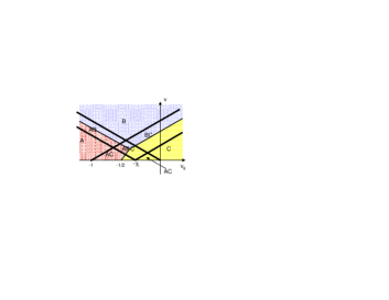
Figure 1: Regions in the $v-v_{g}$ plane of existence of the minima of $U_{eff}$ for $\tilde{\Gamma}\rightarrow 0$. The letters $A$, $B$, and $C$ stand for the presence of a minimum at $y=-1$, $-\gamma_{L}$, and 0, respectively. The plane is separated into three dashed regions according to which of the three extrema is the absolute minimum.

For finite value of $\Gamma$ the stability diagram changes, the main difference is the increase of the region of sequential tunneling that extends towards the axis $v=0$, as shown in Fig. 2.

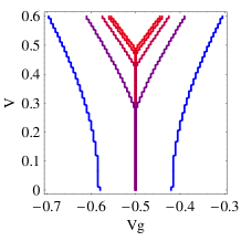
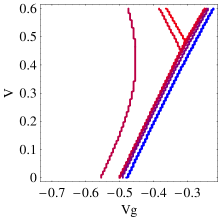
Figure 2: Regions of stability of the sequential tunneling solution for $\gamma_{L}=1/2$ (left panel) and $\gamma_{L}=0.1$ (right panel), and $\tilde{\Gamma}=0.02$, 0.04, 0.08, 0.16, and 0.30, (from red to blue). The region of sequential tunneling evolves from the small triangular shape in the top of the plot (for $\tilde{\Gamma}$ small) to a large trapezoidal shape (for large $\tilde{\Gamma}$) that touches the $v=0$ axis. The regions to the left and the right of the sequential tunneling are “blocked” in the 0 or 1 occupation state, respectively.

At low voltage and small $\tilde{\Gamma}$ one of the two blocked states has the minimum energy. For $\gamma_{L}=\gamma_{R}=1/2$ and $v_{g}=-1/2$ the effective temperature of these states vanishes linearly with the bias voltage. Thus for $v\rightarrow 0$ these are the “cold” states. The effective temperature at the sequential tunneling minimum ($x=-1/2$) is $T^{*}=\pi v^{4}/2^{4}/\tilde{\Gamma}$, thus for small $\tilde{\Gamma}$ this state is always “hot.” Around $v=1/2$ the hot sequential tunneling state becomes the $U_{eff}$ minimum, and the system starts to fluctuate between the hot and cold states. The dimensionless current $\tilde{I}=I/\Gamma e$ in the cold state is very small $\sim\tilde{\Gamma}v$ while in the sequential tunneling regime it is of the order one. The fluctuations between these two states produces large telegraph current noise, as discussed for small $v$ in Ref. MHM, .

The fact that the effective noise temperature varies as a function of the position can lead to dramatic consequences. In the conventional equilibrium statistical mechanics, according to the Gibbs distribution, the lowest energy state is the most probable one. However, if the noise temperature varies as a function of position, it may happen that the lowest energy state, if it experiences higher temperature, may be less likely than a higher energy state that experiences lower temperature. We illustrate this point in Fig. 3, which compares the naive effective potential profile $U_{eff}$ with the actual self-consistent probability distribution.

We need to stress here, however, that we assume that the only environment that is experienced by the mechanical mode so far is the non-equilibrium electronic bath due to the attached leads. If the dominant environment were extrinsic (non-electronic), with a fixed temperature and the coupling strength, then the effective potential would indeed uniquely determine the probabilities of particular states. We will come back to this point in Section VIII.

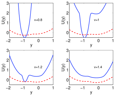
Figure 3: Effective potential $U_{eff}(y)$ (red dashed) compared to $u_{eff}=-\ln{\cal P}(y)$ (blue) for $\tilde{\Gamma}=0.08$, $\gamma_{L}=0.1$, $\tilde{\omega}=10^{-3}$,$v_{g}=0$ and different values of $v$ as indicated in the panes. The quantity $u_{eff}$ plays the role of an effective potential if $T^{*}$ was constant. Note in particular the case $v=1.2$ for which the absolute minimum of $U_{eff}$ is not the absolute minimum of $u_{eff}$ due to the fact that $T^{*}$ is much lower in the other minimum.

In order to discuss the behavior of the device in the full range of parameters here we resort to a numerical solution of the Fokker-Plank equation from which we can determine both the current and the current noise of the device. In the following section we discuss the numerical results.

V Numerical Results for the Current and zero-frequency Noise

The expressions (15), (17) and (24) can be used to calculate the current and the noise of the device. In general the analytical evaluation of these expressions is not possible. Numerically, the solutions can be obtained by rewriting Eq. (12) on a discrete lattice $(x,p)$ and replacing the derivatives with their finite differences approximations. If the equation is solved in a sufficiently large (e.g. rectangular) region in the $x$-$p$ plane, one can use vanishing boundary conditions, since the probability vanishes far from the origin. The matrix corresponding to the discretized Fokker-Plank operator ${\cal L}$ is very sparse and the numerical solution is relatively easy for matrices of dimensions up to $10^{5}$. The discretization step sizes $k\Delta x/\lambda$ and $\Delta pk/\lambda\omega_{0}m$ must be smaller than $\hbar\Gamma/E_{P}$ in order to have a good convergence. This practically limits our numerical procedure to values of $\hbar\Gamma/E_{p}>0.01$.

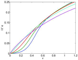
Figure 4: Current for $\tilde{\Gamma}=$ 0.02, 0.04, 0.08, 0.16, and 0.30, from the lowest to the highest curve at low bias. The other parameters are $\tilde{\omega}=10^{-3}$, $\gamma_{L}=1/2$, and $v_{g}=-0.5$.

We begin by considering the symmetric case, $\gamma_{L}=1/2$. The current as a function of the voltage bias for different values of $\tilde{\Gamma}$ is shown in Fig. 4. One can see that for $\tilde{\Gamma}\rightarrow 0$ the current is suppressed for $v<1/2$ and rises very rapidly for transport voltages exceeding the threshold, as expected from the qualitative arguments given above. Numerically is difficult to reduce $\tilde{\Gamma}$ further, but we expect that for $\tilde{\Gamma}\rightarrow 0$ a discontinuity should appear as found in the case when cotunnelling is negligible.fabio

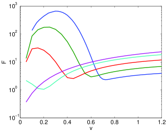
Figure 5: Fano factor of the current noise in logarithmic scale for $\tilde{\Gamma}=$ 0.02, 0.04, 0.08, 0.16, and 0.30, from the lowest to the highest curve at large bias. $\tilde{\omega}=10^{-3}$, $\gamma_{L}=1/2$ and $v_{g}=-0.5$.

In Fig. 5 we plot on a log scale the Fano factor [$F=S(\omega=0)/2eI$] of the mechanically generated current noise (the standard shot noise contribution is much smaller). One can see that $F$ reaches huge values of the order of $10^{3}$, while it is typically 1 for the purely electronic devices. The maximum of the Fano factor appears slightly below the value of the voltage where there is a crossover from the the cold to the hot minima; we will see later that this corresponds to the value for which the switching rates between the two minima are nearly the same. Since the blocked minimum is colder than the sequential tunneling minimum, this crossover happens before the hot minimum becomes a true minimum. Enhancement of noise in this device should serve as a strong indication of the presence of mechanical oscillations.

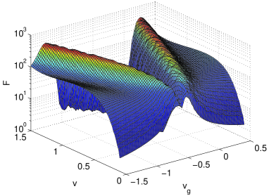
Figure 6: Symmetric case. Fano factor for the induced current noise as a function of $v_{g}$ and $v$ for $\tilde{\Gamma}=0.08$, $\gamma_{L}=0.5$ and $\tilde{\omega}=10^{-3}$.

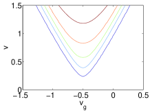
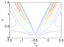
Figure 7: Symmetric case. Current and Fano factor for the mechanically induced current noise as a function of $v_{g}$ and $v$ for $\tilde{\Gamma}=0.08$, $\gamma_{L}=0.5$ and $\tilde{\omega}=10^{-3}$.

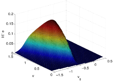
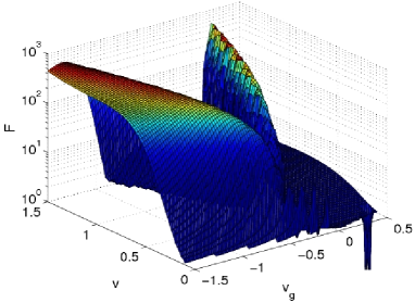
Figure 8: Asymmetric case. Fano factor for the mechanically induced current noise as a function of $v_{g}$ and $v$ for $\tilde{\Gamma}=0.08$, $\gamma_{L}=0.1$ and $\tilde{\omega}=10^{-3}$.

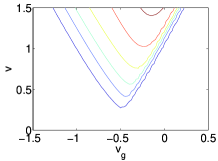
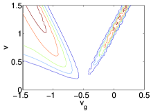
Figure 9: Asymmetric case. Current and Fano factor for the mechanically induced current noise as a function of $v_{g}$ and $v$ for $\tilde{\Gamma}=0.08$, $\gamma_{L}=0.1$ and $\tilde{\omega}=10^{-3}$.

In Fig. 6, 7, 8 and 9 we show the behavior of the Fano factor in the plane $v_{g}-v$ for $\tilde{\Gamma}=0.08$ and $\gamma_{L}=0.5$ or 0.1. Note that in the asymmetric case, Fig. 8 and 9, there is a very sharp peak in the Fano factor if we increase the bias voltage at fixed gate voltage greater than zero. This structure appears at the threshold of the sequential tunnelling conducting region.

VI switching rate

In the previous sections we have studied the current and the current noise. These quantities are the most readily accessible in transport measurements; however, it is interesting also to investigate what is the typical switching time $\tau_{s}$ between the two minima. This quantity can give an indication if the telegraph noise could be detected directly as a slow switching between discrete values of the average current. For this to happen the switching time must be very long–at least comparable to the average current measurement time (typically, in the experiment $\gtrsim 1\ \mu$s) .

To find a reliable estimate of $\tau_{s}$ we need to know the typical time necessary for the system to jump from a local minimum of the effective potential Eq. (30) to a neighboring one. This concept is well defined since the diffusion and damping term of the Fokker-Plack equation are very small and the time evolution of the system on a short time scale is controlled by the drift term. Let us denote the value of the effective potential at the local maximum separating the two minima of interest as $E_{max}$. The region $\Omega$ on the $y$-$q$ plane around the minimum defined by $E_{min}<E_{eff}(y,q)<E_{max}$ can be considered as the trapping region. If the system is at time 0 at the position $(y,q)$ inside $\Omega$ we can estimate the average time to reach the boundary of $\Omega$ ($\partial\Omega$) by solving the equation:

$${\cal L}^{\dagger}\tau=-1$$ (34)

with (absorbing) vanishing boundary conditions on $\partial\Omega$.BookFP Here $\tau$ stands for the function $\tau(y,q)$. Since we are interested on the average time to leave the region we average the escape time with the quasi-stationary distribution function. The vanishing boundary conditions introduce a sink thus there is no zero eigenvalue for the ${\cal L}$ operator with vanishing boundary conditions on $\partial\Omega$. We can nevertheless always identify the eigenvalue with the smallest real part and call it $\lambda_{0}$: ${\cal L}v_{0}=\lambda_{0}v_{0}$. We thus obtain

$$\left\langle\tau\right\rangle\equiv{(\tau,v_{0})\over(1,v_{0})}=-{1\over\lambda_{0}}\,.$$ (35)

The inverse of the lowest eigenvalue gives the average switching time; this is not surprising since the time evolution of the eigenstate $v_{0}$ is $e^{-t\lambda_{0}}$. It decays exponentially on a time scale $-1/\lambda_{0}$ due to the escape at the boundaries of the region $\Omega$.

We implemented numerically the calculation by solving the Fokker-Planck equation in the energy-angle coordinates. If $(y_{o},0)$ is a minimum of the effective potential with energy $E_{min}$, we rewrite the Fokker-Planck equation in terms of the variables $E(x,q)=q^{2}/2+U_{eff}(x)$ and $\theta(x,q)=\arctan(q/(x-x_{o}))$. In this way the boundary conditions read ${\cal P}(E=E_{max},\theta)=0$ for all values of $\theta$. The results are shown in Figs. 10 and 11 for the symmetric and asymmetric case, respectively.

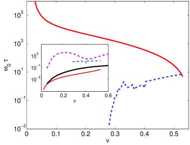
Figure 10: Symmetric case. $\gamma_{L}=1/2$, $\tilde{\Gamma}=0.08$, $v_{g}=-1/2$ and $\tilde{\omega}=10^{-3}$. Switching time between the two minima: red full line for the blocked transport minima ($y=0$ or $y=-1$), and blue dashed line for the sequential tunneling minimum. In the inset: the current in each minimum (same notation of main plot) the average current (black full line) and the current noise (magenta dashed line).

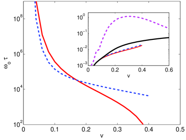
Figure 11: Asymmetric case. $\gamma_{L}=0.1$, $\tilde{\Gamma}=0.08$, $v_{g}=-1/2$, and $\tilde{\omega}=10^{-3}$. Same notations as as in Fig. 10.

Let us begin by discussing the symmetric case of Fig. 10. For small bias voltage only two minima are present, they are perfectly symmetric and they correspond to two “blocked” (classically-forbidden) current state with $n=0$ or 1. The switching time is very long, and the system switches between two blocked states, each with very small cotunneling currents. Since the cotunneling currents for both minima in the symmetric state are the same, there is no telegraph noise for small $v$. As it can be seen from the value of result for the noise, the current fluctuations are nevertheless high, and the reason is that to jump from one minimum to the other the system has to pass through a series of states for which current flows through the device is significant. Moreover the slow fluctuations of the distribution function inside each minimum are important for the noise as discussed in the following Section VII. The fact that the jumping times are so long may actually hinder the observation of the jumps in a real experiment with finite measurement time. In a real device then the noise could be smaller in that case. Increasing the voltage to $v\approx 0.28$, the sequential tunneling minimum at $x=-.5$ appears and a true telegraph noise start to be present. We see very clearly this in the escape times, which are no longer symmetric (we plot the $y=-1$ and $y=-1/2$ minima escape times, the $y=0$ minimum has the same behavior of the $y=-1$ minimum), and the average current at the minima also changes abruptly. Even if the noise has a strong maximum near $v=0.28$ there is not a dramatic increase at the appearance of the minimum. The presence of the cotunneling smoothes the transition also for the noise that has its maximum before the sequential minimum appears. The switching time changes by 6 orders of magnitude in a very small range of bias voltage. Above $v\approx 0.53$ only the sequential tunneling minimum survives.

We consider now the asymmetric case of Fig. 11. It is clear that the evolution of the escape times is very different from the symmetric case. In particular we consider the strongly asymmetric case of $\gamma_{L}=0.1$. In this case the sequential tunneling minimum merges with the blocked $n=0$ minimum, leading to a two minima landscape of the potential. The consequence is that there is no abrupt appearance of a new minimum for some value of the bias voltage; rather, the two minima are always present at the same time till $v\approx 0.4$. At low voltage the potential landscape is nearly symmetrical, both minima are cold, but for the sequential tunneling one is characterized by a slightly higher $T^{*}$ and thus its escape time is shorter (dashed line in Fig. 11). Increasing the voltage, the height of the potential barrier for the blocked state reduces, thus reducing the escape time. At some point (in the case of Fig. 11 for $v\approx 0.18$) the escape time from the cold state become shorter than the escape time of the hot one, since the the temperature has to be compared with the barrier, and at this point the barrier height is smaller in the cold state. Near the crossing region the noise shows a maximum, due to the fact that the system spends nearly half of his time in each of the two minima, with different average current. Tuning $v$ one can thus cross from a region where the system is trapped in one of the two minima, to a region where it jumps on a relatively long time scale from one minimum to the other. If the switching time scale becomes of the order of the response time of the measuring apparatus it is in principle possible to observe directly the fluctuation between the two values of the current.

This is even more pronounced if we follow the evolution of the current at $v_{g}=0$. As can be seen in the contour plot of the Fano factors (cfr. Fig. 9), in this way we will cross a very sharp peak of the Fano factor. The results are shown in Fig. 12. At low voltage only a single nearly blocked state is present ($x=-1$ and $n=1$). For $v\approx 0.8$ a new minimum appears at $x\approx-\gamma_{L}=-0.1$ that is for the moment at higher energy and with a very small barrier. The current associated to this minimum is much higher than the other, and the system starts to switch between the two states. The switching is very slow thus the noise is high. Very rapidly as a function of $v$ the new local minimum becomes the true minimum, and then the other minimum disappears.

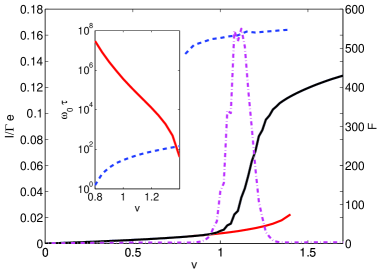
Figure 12: Average Current (black continuous line), Fano factor (magenta dot-dashed line), current in the two minima (same notation as Fig. 10) for $\tilde{\Gamma}=0.08$, $\gamma_{L}=0.1$, $\tilde{\omega}=10^{-3}$ at $v_{g}=0$. In the inset the escape times from the two minima as a function of the bias voltage $v$.

VII Frequency-dependence of the current noise

Eq. (24) derived above can be applied to study not only the zero frequency noise, $S(\omega=0)$, and the Fano factor, as we did in Section V, but also the current noise at an arbitrary frequency. In this section we numerically evaluate $S(\omega)$ and provide a qualitative explanation for the observed trends. As we mentioned before, the shot noise contribution to the noise can be neglected as far as the frequency considered is much smaller than $\Gamma$. From the numerical calculations we find that the frequency dependence is characterized by a single frequency scale, and approximately is Lorentzian peaked at $\omega=0$. This can be seen in the inset of Fig. 13 where we show $S(\omega)$ as a function of $\omega/\omega_{0}$ on a logarithmic scale for several values of the bias voltage $v$. One can parameterize each curve by a single number, that we choose as the frequency $\omega_{c}$ at which $S(\omega_{c})=S(0)/2$. It is instructive to compare the time scale $1/\omega_{c}$ with the energy dissipation and the switching timescales in various regimes.

At low voltages, since switching between the metastable minima is exponentially slow, we anticipate that the low frequency ($\omega<\omega_{0}$) current fluctuations will be determined by the energy fluctuations within the single well in which the molecule spends most of its time. For a simple harmonic oscillator, the corresponding time scale is given by the inverse damping coefficient. For small energy fluctuations, the current changes with energy linearly. Thus, current fluctuations will track the energy fluctuations, i.e. will be Lorentzian with the width given by $A/m$. To check this we plotted in Fig. 13 the value of $m\omega_{0}/A(x)$ evaluated at the minimum of the potential (dotted line). There is a reasonable agreement for low voltage but, as expected, not for large voltages. The reason is that at large $v$ the system becomes hot, and the energy dependence of $A$ cannot be neglected. To address this issue, we calculated the average of $A(x)$ with the distribution function ${\cal P}(x)$ obtained by solving numerically the stationary problem. The result using thus obtained $A$ is shown as dashed line on the figure. We find that it agrees very well with the $\omega_{c}$ extracted from the numerical calculation of $S(\omega)$, both at high and low voltages. Note that at high voltage the energy dependence of $A$ is crucial to understand the frequency response of the noise. The effective temperature changes the average of $A$, and hence $\omega_{c}$ by nearly three orders of magnitude.

In the intermediate transport voltage regime, $1<v<1.3$, the system switches between the two wells frequently. Therefore, we naturally expect that the timescale for the current noise should depend on the switching rate between the wells. If each of the wells would corresponds to a fixed value of current the resulting noise would be a telegraph, with the Lorentzian lineshape and width given by the sum of the switching rates. However, in each well as a function of energy current is not fixed. In fact, the current increases gradually in the “blocked” well as the energy the approaches the top of the barrier reaching the value $I\sim\Gamma$ near the top of the barrier. On the other hand, in the well where transport is sequential, current remains approximately $I\sim\Gamma$ for any energy. Therefore, one can naturally expect deviations from the simple telegraph behavior. Indeed, we find that the timescale $1/\omega_{c}$ tracks the escape time from the “blocked” well (blue dot-dashed line in Fig. 13), which is the longer escape rate, and the fast escape from the “hot” sequential well does not matter. We therefore conclude that the noise is governed by the energy (and thus current) fluctuations within the cold (more probable) well, which also occur on the timescale comparable to the escape rate from it.

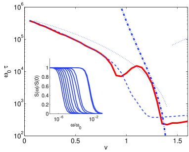
Figure 13: Inset: Frequency dependence of the current noise for several values of the bias voltage. From this data we estracted $\omega_{c}$ as the frequency at which $S(\omega_{c})=S(0)/2$. Main plot: comparison of $\omega_{0}/\omega_{c}$ red full line, the escape time $\omega_{0}\tau$ blue dot-dashed line, the friction coefficient $\omega_{0}m/A$ at the minimum dot line, and averaged light dashed line. The parameters are the same as Fig. 12.

VIII role of extrinsic environmental dissipation

As we discussed above most of the effects we found are due to the non-equilibrium dynamics of the oscillator. In order to improve our understanding of this fact, and to probe robustness of the results to external perturbations we consider the influence of extrinsic dissipation on the system. This can be easily included in the model since the coupling to an external bath implies only additional dissipation and fluctuation on top of the intrinsic ones. We assume that the system is damped due to the coupling to an external bath at equilibrium at the temperature $T_{b}$. The fluctuation and dissipation coming from this coupling satisfy the fluctuation dissipation theorem. Thus the presence of the extrinsic damping induces the following change in the variables $A$ and $D$ defined in Eqs. (10) and (11): $A\rightarrow A+\eta$ and $D\rightarrow D+k_{B}T_{b}\eta/2$. We present the numerical results for the dimensionless parameters $\tilde{\eta}=\eta/m\omega_{0}$ and $\tilde{T}_{b}=2k_{B}T/E_{P}$. The numerical procedure remains unchanged.

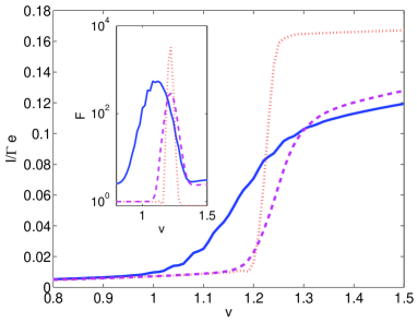
Figure 14: Voltage dependence of the current and Fano factor (inset) for different values of the extrinsic dissipation: $\tilde{\eta}=0$, $10^{-3}$ and $0.1$. The temperature of the external bath is $0.01$ in our dimensional units, the other parameters are the same as Fig. 12. One can see that the current jump becomes sharper for stronger coupling to the environment. At the same time the Fano factor becomes sharper, thus a strong noise region survives, but becomes very narrow when the external bath dominates.

We show in Fig. 14 the behavior of the current and the noise for the same parameters of Fig. 12 but at $\tilde{T}_{b}=0.01$ and for different values of the external dissipation. The main feature that can be clearly seen is the sharpening of the step for the current. The external damping reduces the position fluctuations of the oscillator thus reducing its ability to escape from the blocked regions of the parameters’ space. On the other side if the oscillator is in a conducting region the probability that it can fluctuate to regions of blocked transport is smaller, thus the current is increased in the conducting regions and reduced in the blocked regions, increasing the steepness of the step. For the same reason the region of large noise is reduced. We find that the value of the Fano factor remains actually very large, but only in a very narrow range of bias voltages. Increasing the coupling to the external bath reduces this windows and thus finally rule out the possibility of observe it at all.

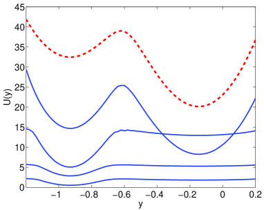
Figure 15: Effective potential $U_{eff}$ (red dashed) compared to $-\ln({\cal P}(x))$ for different values of the extrinsic dissipation: $\tilde{\eta}=10^{-5}$, $10^{-3.5}$, $10^{-2}$, and $10^{-0.5}$, from the lowest to the highest curve. The temperature of the external bath is $0.01$ in our dimensional units, the other parameters are the same as Fig. 12 and the curves are shifted and multiplied by a constant factor for clarity.

A second interesting quantity to study is the distribution function ${\cal P}(x)$. If the coupling to the environment dominates we expect that ${\cal P}(x)={\rm const}\,e^{-U_{eff}(x)/\tilde{T}_{b}}$ to verify this fact we compare ${\cal U}(x)=-\ln{\cal P}(x)$ and $U_{eff}(x)$ in Fig. 15. We find that for small coupling first ${\cal U}(x)$ deviates even more from the form of $U_{eff}$: the minimum in the cold regions deeps (left minimum in the figure). The reason is that the increase of the damping is more effective in the cold region where both of damping and fluctuation are small. In the hot region (right minimum in the figure) the intrinsic fluctuation and dissipation is very large and for small external damping there is no noticeable effect. Increasing the coupling to the environment also the hot minimum is cooled and the shape of $\cal U$ becomes similar to that of $U_{eff}$ shown dashed in the plot. This shows how relevant the non-equilibrium distribution of the position is for the determination of the transport properties of the device.

IX conclusions

In this work our goal was to provide a unified description of the transport properties of the strongly coupled non-equilibrium electron-ion system mimicking a molecular device, in a broad range of parameters. Our results are based on a controlled theoretical approach, which only assumes that the vibrational frequency is the lowest energy scale in the problem. In this regime, the vibrational mode experiences the effect of the electronic environment as a non-linear bath that has three interrelated manifestations: (1) Modification of the effective potential, including formation of up to two additional minima, (2) position-dependent force noise that drives the vibrational mode, and finally, (3) position-dependent dissipation. We have self-consistently included the effect of tunneling electrons on the dynamics of the vibrational mode, and the inverse effect of the vibrational mode on the electron transport. This enabled us to obtain the average transport characteristic of the “device,” i.e. the dependence of the current on the transport and gate voltages, as well as address the problem of current noise and mechanical switching between the metastable states. The agreement between the switching dynamics and the frequency dependence of the current noise determined independently, enabled us to construct a comprehensive but simple understanding of the combined electron-ion dynamics in different transport regimes. In particular, the enhancement of current noise may serve as an indicator of generation of mechanical motion, and its magnitude and frequency dependence provide information on the regime the molecular switching device is in and the values of relevant parameters.

References

- (1) M. A. Reed and J. M. Tour, Sci. Am. 282, 86 (2000); A. Nitzan and M. A. Ratner, Science 300, 1384 (2003).
- (2) K. K. Likharev and D. B. Strukov, in: Introduction to Molecular Electronics, pp. 447-477, G. Cuniberti et al. (eds.), (Springer, Berlin, 2005),
- (3) J. E. Green, J. W. Choi, A. Boukai, Y. Bunimovich, E. Johnston-Halperin, E. DeIonno, Y. Luo, B. A. Sheriff, K. Xu, Y. S. Shin, H.-R. Tseng, J. F. Stoddart, and J. R. Heath, Nature 445, 414 (2007).
- (4) A. Aviram and M.A. Ratner, Chem. Phys. Lett. 29, 277 (1974).
- (5) R. F. Service, Science 302, 556 (2003); J. R. Heath, J. F. Stoddart, R. S. Williams, E. A. Chandross, P. S. Weiss, and R. Service, Science 303, 1136 (2004).
- (6) X. D. Cui, A. Primak, X. Zarate, J. Tomfohr, O. F. Sankey, A. L. Moore, T. A. Moore, D. Gust, G. Harris, and S. M. Lindsay, Science 294, 571 (2001); W. Wang, T. Lee, and M. A. Reed, Phys. Rev. B 68, 035416 (2003); X. Xiao, B. Xu, and N. Tao, Nano Lett. 4, 267 (2004).
- (7) M. Di Ventra, S. T. Pantelides, and N. D. Lang, Phys. Rev. Lett. 84, 979 (2000); Y. Hu, E. Zhu, H. Gao, and H. Guo, Phys. Rew. Lett. 95, 156803 (2005); D. M. Cardamone and G. Kirczenow, Phys. Rev. B 77, 165403 (2008).
- (8) C. Li, D. Zhang, X. Liu, S. Han, T. Tang, C. Zhou, W. Fan, J. Koehne, J. Han, M. Meyyappan, A. M. Rawlett, D. W. Price, and J. M. Tour, Appl. Phys. Letters 82, 645 (2003); A. S. Blum, J. G. Kushmerick, D. P. Long, C. H. Patterson, J. C. Yang, J. C. Henderson, Y. Yao, J. M. Tour, R. Shashidhar, and B. R. Ratna, Nature Materials 4, 167 (2005); R. A. Kiehl, J. D. Le, P. Candra, R. C. Hoye, and T. R. Hoye, Appl. Phys. Lett. 88, 172102 (2006); E. Lörtscher, J. W. Ciszek, J. Tour, and H. Riel, Small 2, 973 (2006).
- (9) S. Braig and K. Flensberg, Phys. Rev. B 68, 205324 (2003).
- (10) J. Koch and F. von Oppen, Phys. Rev. Lett. 94, 206804 (2005).
- (11) M. Galperin, M.A. Ratner, and A. Nitzan, Nano Letters 5, 125 (2005).
- (12) D. Mozyrsky, M.B. Hastings, and I. Martin, Phys. Rev. B 73, 035104 (2006).
- (13) J. Park, A. N. Pasupathy, J. I. Goldsmith, C. Chang, Y. Yaish, J. R. Petta, M. Rinkoski, J. P. Sethna, H. D. Abruña, P. L. McEuen, and D. C. Ralph, Nature (London) 417, 722 (2002).
- (14) L. H. Yu and D. Natelson, Nano Lett. 4, 79 (2004).
- (15) H. Park, J. Park, A. K. L. Lim, E. H. Anderson, A. P. Alivisatos, and P. L. McEuen, Nature (London) 407, 57 (2000).
- (16) N. B. Zhitenev, H. Meng, and Z. Bao, Phys. Rev. Lett. 88, 226801 (2002).
- (17) X. H. Qiu, G. V. Nazin, and W. Ho, Phys. Rev. Lett. 92, 206102 (2004).
- (18) D.-H. Chae, J. F. Berry, S. Jung, F. A. Cotton, C. A. Murillo, and Z. Yao, Nano Lett. 6, 165 (2006).
- (19) S. Sapmaz, P. Jarillo-Herrero, Ya. M. Blanter, C. Dekker, and H. S. van der Zant, Phys. Rev. Lett. 96, 026801 (2006).
- (20) D. Boese and H. Schoeller, Europhys. Lett. 54, 668 (2001).
- (21) V. Aji, J.E. Moore, and C.M. Varma, cond-mat/0302222 (2003).
- (22) A. Mitra, I. Aleiner, and A. J. Millis, Phys. Rev. B 69, 245302 (2004).
- (23) A. Armour, M. Blencowe, and A. Zhang, Phys. Rev. B 69, 125313 (2004).
- (24) C. B. Doiron, W. Belzig, and C. Bruder, Phys. Rev. B 74, 205336 (2006).
- (25) F. Pistolesi and S. Labarthe, Phys. Rev. B 76 165317 (2007).
- (26) J. P. Paz and W. H. Zurek, Phys. Rev. Lett. 82, 5181 (1999).
- (27) I. Martin and W. H. Zurek, Phys. Rev. Lett. 98, 120401 (2007).
- (28) Ya. M. Blanter, O. Usmani, and and Yu. V. Nazarov, Phys. Rev. Lett. 93, 136802 (2004), ibid 94, 049904 (2005); O. Usmani, Ya. M. Blanter, and Yu. V. Nazarov, Phys. Rev. B 75, 195312 (2007).
- (29) J. Koch, F. von Oppen, and A.V. Andreev, Phys. Rev. B 74, 205438 (2006).
- (30) R. Aguado and L. P. Kouwenhoven, Phys. Rev. Lett. 84, 1986 (2000).
- (31) C. W. Gardiner, Quantum Noise (Springer-Verlag, 1991).
- (32) A.A. Clerk and S. Bennett, New J. Phys. 7, 238 (2005).
- (33) G.B. Lesovik, Soviet. JETP Lett. 49, 592. (1989); M. Büttiker, Phys. Rev. B 46, 12485 (1992).
- (34) F. Pistolesi, Phys. Rev. B 69, 245409 (2004).
- (35) Nonequilibrium Statistical Mechanics, R. Zwanzig (Oxford University Press, New York, 2001).