Channeling of Protons Through Carbon Nanotubes Embedded in Dielectric Media

Abstract

We investigate how the dynamic polarization of the carbon atoms valence electrons affects the spatial distributions of protons channeled in the (11, 9) single-wall carbon nanotubes placed in vacuum and embedded in various dielectric media. The initial proton speed is varied between 3 and 8 a.u., corresponding to the energies between 0.223 and 1.59 MeV, respectively, while the nanotube length is varied between 0.1 and 0.8 $\mu$m. The spatial distributions of channeled protons are generated using a computer simulation method, which includes the numerical solving of the proton equations of motion in the transverse plane. We show that the dynamic polarization effect can strongly affect the rainbow maxima in the spatial distributions, so as to increase the proton flux at the distances from the nanotube wall of the order of a few tenths of a nanometer at the expense of the flux at the nanotube center. While our findings are connected to the possible applications of nanosized ion beams created with the nanotubes embedded in various dielectric media for biomedical research and in materials modification, they also open the prospects of applying ion channeling for detecting and locating the atoms and molecules intercalated inside the nanotubes.

Keywords: nanotubes, channeling, dynamic polarization, rainbows

1 Introduction

Theoretical modeling of ion channeling through carbon nanotubes has reached a mature level [1, 2, 3] whereas experimental realization of this process is still at the preliminary stage [4, 5]. Nevertheless, theoreticians continue to explore possible applications of ion channeling through the nanotubes, beginning with those based on the angular distributions of channeled ions, e.g., for the purpose of deflecting ion beams in accelerators [6, 7] or determining some structural details of the short nanotubes using the rainbow effect [8, 9, 10, 11]. Besides, theoretical studies of the spatial distributions of channeled ions have demonstrated the possibility of creating nanosized ion beams, which could find interesting applications in biomedical research and for materials modification [6, 12, 13, 14, 15]. However, an additional application of ion channeling through the nanotubes based on the spatial distributions remains to be investigated in the context of extending the classical use of ion channeling for materials analysis [16] to the nanotube based materials.

Namely, one of the most powerful applications of ion channeling through single crystals was developed to detect and locate their defects. It is based on measuring ion dechanneling on such defects in combination with their Rutherford backscattering [16]. It was crucial for this application of ion channeling to develop the adequate theoretical models for calculating the spatial distributions of channeled ions, and thus enable the precise control and interpretation of the measurements, providing the information on such defects [16]. On the other hand, the nanotubes can exhibit numerous defects, appearing during their synthesis or due to external agents such as particle irradiation [17]. Moreover, one of the main directions within the nanotube research is related to the phenomena of intercalation of the atomic and molecular species in them [18]. Therefore, it is reasonable to explore whether ion channeling can be also used to analyze defects in the nanotubes, in particular, to detect and locate the atoms and molecules intercalated in them. In a first attempt to address this problem, we present here a detailed study of the spatial distributions of protons channeled through the nanotubes, with special emphasis on the rainbow effect in the transverse plane with its possible applications.

Having in mind that the ion channeling regime is most suitable for probing the atoms intercalated in the nanotubes involves light ions in the MeV energy range [16], one must emphasize that, for such projectiles, the dynamic polarization of the nanotube atoms valence electrons can give rise to the strong image force, which can pull the channeled ions towards the nanotube wall [19]. Of course, one expects that the intercalated atoms would be placed right there, close to the nanotube wall, in some state of adsorption on the nanotube atoms surface. While the image force has not been found to play any significant role in channels of single crystals [16], its role has been identified clearly in ion-surface scattering [20], and in ion transmission through capillaries in solids [21, 22]. In addition, although the image force plays the minor roles in ion channeling through the nanotubes in the GeV and keV energy ranges [1, 2, 6, 7, 23], it has been shown to influence strongly ion trajectories in the MeV energy range. For example, the image force gives rise to the rainbow effect in angular distributions of protons channeled through the short chiral single-wall and double wall nanotubes [24, 25].

It has been established that, when the nanotubes are grown in a dielectric medium, one can achieve a very high degree of their ordering and straightening. This makes such composite structures very suitable candidates to be used in experiments of ion channeling through the nanotubes. Therefore, it is important to study the effects of the surrounding dielectric medium on ion channeling through the nanotubes in the MeV energy range. The materials of interest are Al₂O₃ [4], SiO₂ [26, 27] as well as Ni [28] and Pt [5]. In this context, it has been shown recently that the image force and, consequently, the rainbow effect in the angular distributions of protons channeled through the nanotubes can be strongly modified by the polarization of the surrounding cylindrical dielectric boundary [29, 30]. The separation between the nanotube and the SiO₂ and Al₂O₃ boundaries is approximated by the nanotube atom van der Waals radius [31, 32]. The separation between the nanotube and the Ni boundary is approximated by the separation between the a graphene and a (111) Ni surface, which was calculated using a minimization structural calculation based on the density functional theory [33]. In both cases the obtained separation was 3.21 a.u.

We shall investigate here how the spatial distributions of protons channeled in the (11, 9) single-wall nanotubes placed in vacuum or embedded in various dielectric media are affected by the dynamic polarization effect. While such a study complements our previous studies of the influence of the image force on the rainbow effect in the angular distributions of protons channeled in the nanotubes [24, 25, 30], we expect that the analogous influence on the spatial distribution of channeled protons may lead to a significant change of the proton flux within the nanotube, enabling one to probe the atoms and molecules adsorbed on the nanotube wall. The image force acting on the proton moving through the nanotube embedded in a dielectric medium will be calculated using a two-dimensional hydrodynamic model of the nanotube atoms valence electrons while the surrounding dielectric medium will be described by a suitable dielectric function [29].

After outlining the basic theory used in modeling the interaction potentials between the proton and the nanotube and dielectric medium, we shall discuss the results of the proton trajectory simulations and give the concluding remarks.

The atomic units will be used throughout the paper unless explicitly stated otherwise.

2 Theory

The system under investigation is a proton moving through an (11, 9) single-wall carbon nanotube embedded in a dielectric medium. The $z$ axis coincides with the nanotube axis and the origin lies in its entrance transverse plane. The initial proton speed vector is taken to be parallel to the $z$ axis. We assume that the nanotube is sufficiently short for the proton energy loss to be neglected. The initial proton speed, $v$, is varied between 3 and 8 a.u., corresponding to the energies between 0.223 and 1.59 MeV, respectively. The nanotube length, $L$, is varied between 0.1 and 0.8 $\mu$m.

We assume that the (repulsive) interaction between the proton and nanotube atoms can be treated classically using the Doyle-Turner expression for the proton-nanotube atom interaction potential averaged axially and azimuthally [34, 35, 36]. The resulting interaction potential reads

$$U_{rep}(r)=\frac{16\pi Z_{1}Z_{2}d}{3\sqrt{3}l^{2}}\sum\limits_{j=1}^{4}{a_{j}b_{j}^{2}I_{0}(b_{j}^{2}rd)\exp\{-b_{j}^{2}}[r^{2}+(d/2)^{2}]\},$$ (1)

where $Z_{1}$ = 1 and $Z_{2}$ = 6 are the atomic numbers of the proton and nanotube atom, respectively, $d$ is the nanotube diameter, $l$ is the nanotube atoms bond length, $r$ is the distance between the proton and nanotube axis, $I_{0}$ designate the modified Bessel function of the first kind and the $0^{th}$ order, and $a_{j}=(0.115,0.188,0.072,0.020)$ and $b_{j}=(0.547,0.989,1.982,5.656)$ are the fitting parameters [36].

The dynamic polarization of the nanotube and dielectric medium by the proton is treated using a two-dimensional hydrodynamic model of the nanotube atoms valence electrons, based on a jellium-like description of the nanotube ion cores, extended to include the contribution of the dielectric boundary [37, 19, 29]. This model includes the procedures of axial and azimuthal averaging, as the repulsive interaction model. It gives the (attractive) interaction potential between the proton and its image. Let us designate the proton position at time $t$ by $\vec{r}=\vec{r}(t)$ and the electric potential at point $\vec{R}$ originating from the (screened) proton, perturbing the nanotube and dielectric boundary, by $\Phi_{ext}(\vec{R},\vec{r},t)$. This potential is called the external potential. The image interaction potential at the proton position reads

$$U_{atr}=-\frac{Z_{1}}{2}\Phi_{ind}(\vec{r},t),$$ (2)

where $\Phi_{ind}(\vec{r},t)$ is the electric potential at the proton position originating from the polarization charges induced on the nanotube and dielectric boundary by the (screened) proton. This potential is called the induced potential.

Since the repulsive and attractive interaction potentials are axially symmetric, the initial proton speed vector is parallel to the $z$ axis and the proton is channeled, the cylindrical coordinates of the proton position are $r=r(t)$, $\varphi=\varphi_{0}$ and $z=vt$, where $\varphi_{0}$ is the azimuthal coordinate of the initial proton position. Let us designate the nanotube and dielectric boundary radii by $a=d/2$ and $b$, respectively. Then, the Fourier transform of the external potential at the nanotube or dielectric boundary, i.e., for $R=a$ or $R=b$, is

$$\tilde{\Phi}_{ext}(R,r)=\frac{2\pi Z_{1}}{\varepsilon_{nt}}g(R,r,m,k)\delta(\omega-kv)\exp(-im\varphi_{0})$$ (3)

where $\varepsilon_{nt}=1$ is the dielectric constant of the nanotube background, $m$, $k$ and $\omega$ are the angular oscillation mode, longitudinal wave number and angular frequency of an elementary excitation of the nanotube atoms valence electrons treated as an electron gas, and $g(R,r,m,k)$ is the radial Green’s function.

The Fourier transform of the induced potential at the proton position is

$$\tilde{\Phi}_{ind}(r)=\frac{-a\tilde{n}_{a}}{\varepsilon_{nt}}[g(a,r,m,k) + bg(b,r,m,k)\Re g^{\prime}(b,a,m,k)]$$ (4)

$$+ bg(b,r,m,k)\Re{\tilde{\Phi}_{ext}^{\prime}(b,r)},$$

where

$$\tilde{n}_{a}=\frac{{\tilde{\Phi}_{ext}(a,r)+bg(b,a,m,k)\Re{\tilde{\Phi}_{ext}^{\prime}(b,r)}}}{{\chi^{-1}+(a/\varepsilon_{nt})[g(a,a,m,k)+bg(b,a,m,k)\Re g^{\prime}(b,a,m,k)]}},$$ (5)

$$\chi=\frac{{n_{0}(k^{2}+{{m^{2}}\mathord{\left/{\vphantom{{m^{2}}{a^{2})}}}\right.\kern-1.2pt}{a^{2})}}}}{{\alpha(k^{2}+{m^{2}\mathord{\left/{\vphantom{{m^{2}}{a^{2})}}}\right.\kern-1.2pt}{a^{2})}}+\beta(k^{2}+{m^{2}\mathord{\left/{\vphantom{{m^{2}}{a^{2})}}}\right.\kern-1.2pt}{a^{2})}}^{2}-\omega(\omega+i\gamma)}},$$ (6)

and

$$\Re=\frac{\varepsilon_{\omega}-\varepsilon_{nt}}{4\pi[\varepsilon_{nt}+(\varepsilon_{nt}-\varepsilon_{\omega})kbI_{m}(kb)K^{\prime}_{m}(kb)]};$$ (7)

$\tilde{n}_{a}$ is the Fourier transform of the surface polarization charge density induced at the nanotube, $\chi$ is the response function of the polarization charge induced at the nanotube, $n_{0}$ = 0.428 a.u. is the equilibrium density of the electron gas, $\alpha=\pi n_{0}$, $\beta=1/4$, and $\gamma\to 0^{+}$, $\Re$ is the response function of the polarization charge induced at the dielectric boundary, $\varepsilon_{\omega}$ is the dielectric function of the dielectric medium, and $I_{m}$ and $K_{m}$ designate the modified Bessel functions of the first and second kinds and the $m^{th}$ order, respectively; the derivatives of functions $g(R,r,m,k)$ and $\tilde{\Phi}_{ext}(R,r)$ are taken with respect to their first arguments.

The induced potential at the proton position is

$$\Phi_{ind}(\vec{r},t)=\sum\limits_{m=-\infty}^{m=\infty}{\int\limits_{-\infty}^{\infty}{\frac{dk}{(2\pi)^{2}}}\int\limits_{-\infty}^{\infty}{\frac{d\omega}{2\pi}\exp\left\{{i\left[{m\varphi_{0}-(\omega-kv)t}\right]}\right\}\tilde{\Phi}_{ind}(r)}}.$$ (8)

The total interaction potential between the proton and the nanotube and dielectric medium reads

$$U(\vec{r},t)=U_{rep}(r)-\frac{Z_{1}}{2}\Phi_{ind}(\vec{r},t).$$ (9)

The spatial distributions of channeled protons in the exit transverse plane are generated using a computer simulation method, which includes the numerical solving of the proton equations of motion in the transverse plane. The rectangular coordinates of the initial proton position, $x_{0}$ and $y_{0}$, are chosen randomly from a two-dimensional uniform distribution with condition $r_{\mathrm{0}}=({x_{0}^{2}+y_{0}^{2}})^{\frac{1}{2}}<a-a_{sc}$, where $a_{sc}=\left[{9\pi^{2}/(128\ Z_{2})}\right]^{\frac{1}{3}}a_{0}$ is the nanotube atom screening radius and $a_{0}$ the Bohr radius. We take for the nanotube atoms bond length $l$ = 0.144 nm [38] and obtain for the nanotube radius $a$ = 0.689 nm. The initial number of protons is 3 141 929.

It has been demonstrated that proton channeling in nanotubes can be analyzed successfully via the corresponding mapping of the impact parameter plane to the scattering angle plane [8, 9, 10, 11, 24, 25]. Analogously, we analyze here the mapping of the entrance transverse plane to the exit transverse plane. However, since in the case we investigate the total interaction potential is axially symmetric, the analysis of this mapping can be reduced to the analysis of the mapping of the proton radial axis in the entrance transverse plane to the proton radial axis in the exit transverse plane. Further, we can take that $y_{0}$ = 0 and analyze only the mapping of the $x_{0}$ axis in the entrance transverse plane to the $x_{0}$ axis in the exit transverse plane. The extrema in this mapping are the rainbow maxima or minima, and the corresponding singularities in the spatial distribution of channeled protons are the rainbow singularities.

3 Results and discussion

We shall analyze first the spatial distributions of protons channeled in the (11, 9) carbon nanotubes placed in vacuum. The proton speed will be $v$ = 3 a.u. and the nanotube lengths $L$ = 0.1, 0.2 and 0.3 $\mu$m. For this proton speed the spatial distributions of channeled protons for the nanotubes embedded in a dielectric medium do not differ from the corresponding spatial distributions for the nanotubes placed in vacuum. This part of the study represents a continuation of our previous study of the influence of the dynamic polarization effect on the angular distributions of protons channeled in the (11, 9) nanotubes placed in vacuum [24].

After that, we shall explore the spatial distributions of protons channeled in the (11, 9) nanotubes embedded in SiO₂. The proton speed will be $v$ = 5 a.u. and the nanotube lengths $L$ = 0.3 and 0.5 $\mu$m. For this proton speed the spatial distributions of channeled protons for the nanotubes embedded in a dielectric medium differ from the corresponding spatial distributions for the nanotubes placed in vacuum. This part of the study represents a continuation of our previous study of the influence of the image interaction potential on the angular distributions of protons channeled in the (11, 9) nanotubes placed in SiO₂ [30]. Then, we shall consider the spatial distributions of protons channeled in the (11, 9) nanotubes embedded in SiO₂, Al₂O₃ and Ni. The proton speed will be $v$ = 8 a.u. and the nanotube length $L$ = 0.8 a.u.

The nanotube radius is $a$ = 13.01 a.u. The separation between the nanotube and the dielectric boundaries is 3.21 a.u. Thus, the dielectric boundary radius is $b=a$ + 3.21 a.u. We describe the surrounding SiO₂ by the dielectric constant of 3.9 [39]. The dielectric responses of the surrounding Al₂O₃ and Ni are modeled using the methods described by Arista and Fuentes [21] and Kwei et al. [40], respectively. We have found that in the cases of SiO₂ and Al₂O₃ a proton moving at a speed below about 3 a.u. does not polarize the dielectric media. This means that the dielectric medium is completely screened by the nanotube and does not contribute to the image force. For a proton speed above about 3 a.u. the polarization of the dielectric media occurs. Consequently, the screening of the dielectric medium by the nanotube is incomplete and it influences the image force.

Figure 1(a) shows two spatial distributions of channeled protons along the $x$ axis in the exit transverse plane for the proton speed $v$ = 3 a.u. and the nanotube length $L$ = 0.1 $\mu$m. The nanotube is placed in vacuum. The spatial distributions correspond to the cases without the dynamic polarization effect and with it. In each case the spatial distribution contains a strong central maximum and a pair of prominent peripheral maxima, designated by 1 in the former case and by 1_i in the latter case. In the case with the dynamic polarization effect the central maximum is narrower and weaker than in the case without it. In the former case the peripheral maxima are located at $x=\pm$8.4 a.u., and in the latter case at $x=\pm$10.2 a.u.

Figure 1(b) shows two mappings of the $x_{0}$ axis in the entrance transverse plane to the $x$ axis in the exit transverse plane corresponding to the two spatial distributions of channeled protons shown in Fig. 1(a). One can see that in each case the mapping has two extrema, a maximum and a minimum. The extrema in the mapping without the image interaction potential are designated by 1 and the extrema in the mapping with it by 1_i. In each case the ordinates of the extrema coincide with the abscissae of the maxima in the corresponding spatial distribution. Since the extrema in the mappings are the rainbow extrema, the maxima in the spatial distributions are in fact the rainbow singularities.

Figure 1: (a) Two spatial distributions of channeled protons along the $x$ axis in the exit transverse plane for the proton speed of 3 a.u. and the nanotube length of 0.1 $\mu$m. The nanotube is placed in vacuum. The dashed line corresponds to the case without the dynamic polarization effect and the solid line to the case with it. The size of a bin along the $x$ axis is 0.3 a.u. (b) Two mappings of the $x_{0}$ axis in the entrance transverse plane to the $x$ axis in the exit transverse plane corresponding to the two spatial distributions.

If the spatial distributions of channeled protons shown in Fig. 1(a) are compared with the corresponding angular distributions of channeled protons [24], obtained for the proton speed $v$ = 3 a.u. and the nanotube length $L$ = 0.1 $\mu$m, it is seen that in the former case the rainbow effect is much more pronounced. In this case the rainbow maxima appear even when the image force is not included, unlike in the latter case.

Figure 2(a) shows two spatial distributions of channeled protons along the $x$ axis in the exit transverse plane for the proton speed $v$ = 3 a.u. and the nanotube length $L$ = 0.2 $\mu$m. The nanotube is placed in vacuum. The spatial distributions correspond to the cases without the image force and with it. In the former case the spatial distribution contains a central maximum and two pairs of peripheral maxima, designated by 1 and 2, and in the latter case a central maximum and three pairs of peripheral maxima, designated by 1_i, 2_i and 3_i. In the case with the image force the central maximum is narrower and about two times weaker while the peripheral maxima are more prominent than in the case without it. In the former case the peripheral maxima are located at $x=\pm$7.8 and $\pm$11.7 a.u., and in the latter case at $x=\pm$9.6, $\pm$10.8 and $\pm$12.0 a.u.

Figure 2(b) shows two mappings of the $x_{0}$ axis in the entrance transverse plane to the $x$ axis in the exit transverse plane corresponding to the two spatial distributions of channeled protons shown in Fig. 2(a). It is clear that in the case without the dynamic polarization effect the mapping has four extrema, two maximum and two minima. They are designated by 1 and 2. In the case with the dynamic polarization effect the mapping has six extrema, three maxima and three minima. They are designated by 1_i, 2_i and 3_i. In each case the ordinates of the extrema coincide with the abscissae of the maxima in the corresponding spatial distribution.

Figure 2: (a) Two spatial distributions of channeled protons along the $x$ axis in the exit transverse plane for the proton speed of 3 a.u. and the nanotube length of 0.2 $\mu$m. The nanotube is placed in vacuum. The dashed line corresponds to the case without the dynamic polarization effect and the solid line to the case with it. The size of a bin along the $x$ axis is 0.3 a.u. (b) Two mappings of the $x_{0}$ axis in the entrance transverse plane to the $x$ axis in the exit transverse plane corresponding to the two spatial distributions.

There are two new features in Fig. 2 when it is compared to Fig. 1. First, each of the spatial distributions of channeled protons given in Fig. 2(a) contains a pair of very weak maxima, designated by 2 in the case without the image force and by 3_i in the case with it. They correspond to the very sharp maxima and minima in the mappings given in Fig. 2(b), designated by 2 and 3_i, which lie near the nanotube wall. It is noteworthy that the image force does not change much the positions and shapes of the very weak maxima in the spatial distribution and the very sharp maxima and minima in the mapping. This can be attributed to the dominance of the repulsive interaction potential in the region near the nanotube wall. Second, the spatial distribution given in Fig. 2(a) without the image force included contains one pair of prominent peripheral maxima, designated by 1, like the corresponding spatial distribution given in Fig. 1(a). On the other hand, the spatial distribution given in Fig. 2(a) with the image force included contains two pairs of prominent peripheral maxima, designated by 1_i and 2_i, unlike the spatial distribution given in Fig. 1(a) with the image force included and the spatial distribution given in Fig. 2(a) without the image force included. They correspond to the shallow maxima and minima in the mapping given in Fig. 2(b) with the image force included, designated by 1_i and 2_i, which lie away from the nanotube wall. These maxima demonstrate the presence of the image force.

Figure 3(a) shows two spatial distributions of channeled protons along the $x$ axis in the exit transverse plane for the proton velocity $v$ = 3 a.u. and the nanotube length $L$ = 0.3 $\mu$m. The nanotube is placed in vacuum. The spatial distributions correspond to the cases without the image interaction potential and with it. In the former case the spatial distribution contains a central maximum and three pairs of peripheral maxima, designated by 1, 2 and 3, and in the latter case a central maximum and five pairs of peripheral maxima, designated by 1_i, 2_i, 3_i, 4_i and 5_i. The maxima designated by 2, 3, 4_i and 5_i are very weak. In the case with the image interaction potential the central maximum is much narrower and about three times weaker while the peripheral maxima are much more prominent than in the case without it. In the former case the peripheral maxima are located at $x=\pm$7.5, $\pm$11.1 and $\pm$12.1 a.u., and in the latter case at $x=\pm$8.1, $\pm$9.9, $\pm$10.7, $\pm$11.4 and $\pm$12.2 a.u.

Figure 3: (a) Two spatial distributions of channeled protons along the $x$ axis in the exit transverse plane for the proton speed of 3 a.u. and the nanotube length of 0.3 $\mu$m. The nanotube is placed in vacuum. The dashed line corresponds to the case without the dynamic polarization effect and the solid line to the case with it. The size of a bin along the $x$ axis is 0.3 a.u. (b) Two mappings of the $x_{0}$ axis in the entrance transverse plane to the $x$ axis in the exit transverse plane corresponding to the two spatial distributions.

Figure 3(b) shows two mappings of the $x_{0}$ axis in the entrance transverse plane to the $x$ axis in the exit transverse plane corresponding to the two spatial distributions of channeled protons shown in Fig. 3(a). It is evident that in the case without the image force the mapping has six extrema, three maxima and three minima. They are designated by 1, 2 and 3. In the case with the image force the mapping has 10 extrema, five maxima and five minima. They are designated by 1_i, 2_i, 3_i, 4_i and 5_i. The maxima and minima designated by 2, 3, 4_i and 5_i are very sharp and lie near the nanotube wall.

Figure 4 shows the spatial distributions of channeled protons in the exit transverse plane for the proton speed $v$ = 3 a.u. and the nanotube length $L$ = 0.3 $\mu$m without the dynamic polarization effect and with it. The nanotube is placed in vacuum. The weak azimuthal asymmetry of the spatial distributions would be less pronounced if the initial number of protons were larger.

It is obvious from Figs. 1-3 that for a longer nanotube the image force makes the spatial distributions of channeled protons richer. Figure 4 shows clearly that the image force causes a significant increase of the proton flux near the nanotube wall, in a similar way as it was observed by Zhou et al. [15]. It is important to note that this increase of the proton flux occurs at the distances from the nanotube wall of the order of 0.2 nm, coinciding with the typical separations between the nanotube wall and the atoms that can be adsorbed on them. Therefore, it is evident that the image force makes possible the use of proton channeling for detecting and locating the atoms and molecules adsorbed on the nanotube wall.

Figure 5 gives five proton trajectories in the $xz$ plane for the $x_{0}$ coordinates of the initial proton position corresponding to the five maxima in the spatial distribution of channeled protons given in Fig. 3(a) with the image interaction potential. The analysis shows that these trajectories, which are called the rainbow trajectories, can be classified according to the number of proton deflections within the total interaction potential well [24]. The number of proton deflections determines the order of the rainbow. One can see that trajectory 4_i, corresponding to maximum 4_i in the spatial distribution, includes one proton deflection. Therefore, the rainbow it represents is the primary rainbow. The rainbows represented by trajectories 1_i, 3_i and 5_i, corresponding to maxima 1_i, 3_i and 5_i in the spatial distribution, are the secondary rainbows, and that represented by trajectory 2_i, corresponding to maxima 2_i in the spatial distribution, is the tertiary rainbow.

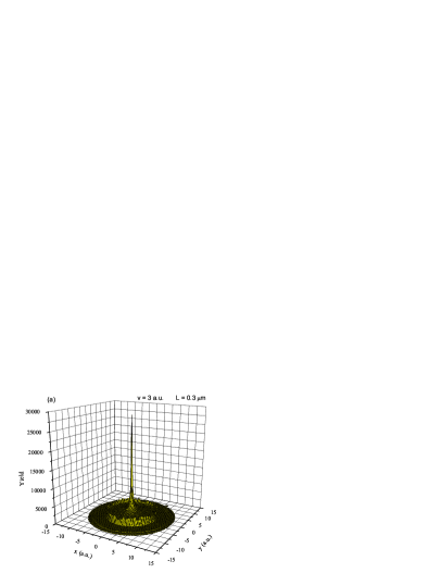
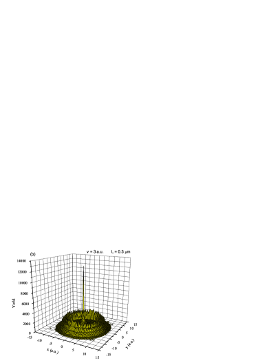
Figure 4: Two spatial distributions of channeled protons in the exit transverse plane for the proton speed of 3 a.u. and the nanotube length of 0.3 $\mu$m. The nanotube is placed in vacuum. The spatial distributions correspond to the cases (a) without the dynamic polarization effect and (b) with it. The sizes of a bin along the $x$ and $y$ axes are 0.3 a.u.

Figure 5: Five proton trajectories in the $xz$ plane for the $x_{0}$ coordinates of the initial proton positions corresponding to the five maxima in the spatial distribution of channeled protons shown in Fig. 3(a) with the dynamic polarization effect included.

We next compare the effects of the image force on the spatial distributions of protons channeled in the nanotube placed in vacuum and embedded in SiO₂. The proton speed is increased to $v$ = 5 a.u. and the nanotube lengths are $L$ = 0.3 and 0.5 $\mu$m.

Figure 6(a) shows two spatial distributions of channeled protons along the $x$ axis in the exit transverse plane for the proton speed $v$ = 5 a.u. and the nanotube length $L$ = 0.3 $\mu$m. They correspond to the cases in which the nanotube is placed in vacuum and embedded in SiO₂. The image force is included. In each case the spatial distribution contains a central maximum and two pairs of peripheral maxima, designated by 1_i and 2_i in the former case, and by 1_d and 2_d in the latter case. The maxima designated by 2_i and 2_d are very weak. In the case in which the nanotube is placed in vacuum the peripheral maxima are located at $x=\pm$9.3 and $\pm$11.9 a.u., and in the case in which it is embedded in SiO₂ at $x=\pm$8.7 and $\pm$11.9 a.u.

Figure 6: (a) Two spatial distributions of channeled protons along the $x$ axis in the exit transverse plane for the proton speed of 5 a.u. and the nanotube length of 0.3 $\mu$m. The dashed line corresponds to the case in which the nanotube is placed in vacuum and the solid line to the case in which it is embedded in SiO₂. The size of a bin along the $x$ axis is 0.3 a.u. (b) Two mappings of the $x_{0}$ axis in the entrance transverse plane to the $x$ axis in the exit transverse plane corresponding to the two spatial distributions.

Figure 6(b) shows two mappings of the $x_{0}$ axis in the entrance transverse plane to the $x$ axis in the exit transverse plane corresponding to the two spatial distributions of channeled protons shown in Fig. 6(a). One can see that in each case the mapping has four extrema, two maxima and two minima. The extrema in the mapping in the case in which the nanotube is placed in vacuum are designated by 1_i and 2_i, and in the case in which it is embedded in SiO₂ by 1_d and 2_d. The maxima and minima designated by 2_i and 2_d are very sharp and lie near the nanotube wall. In each case the ordinates of the extrema coincide with the abscissae of the maxima in the corresponding spatial distribution. Thus, the maxima in the spatial distributions are in fact the rainbow singularities.

Figure 7(a) shows two spatial distributions of channeled protons along the $x$ axis in the exit transverse plane for the proton speed $v=$5 a.u. and the nanotube length $L$ = 0.5 $\mu$m. They correspond to the cases in which the nanotube is placed in vacuum and embedded in SiO₂. The dynamic polarization effect is included. In the former case the spatial distribution contains a central maximum and four pairs of peripheral maxima, designated by 1_i, 2_i, 3_i and 4_i, and in the latter case a central maximum and three pairs of peripheral maxima, designated by 1_d, 2_d and 3_d. The maxima designated by 3_i, 4_i, 2_d and 3_d are very weak. In the case in which the nanotube is placed in vacuum the peripheral maxima are located at $x=\pm$9.0, $\pm$9.9, $\pm$11.2 and $\pm$12.1 a.u., and in the case in which it is embedded in SiO₂ at $x=\pm$9.3, $\pm$11.2 and $\pm$12.1 a.u.

Figure 7: (a) Two spatial distributions of channeled protons along the $x$ axis in the exit transverse plane for the proton speed of 5 a.u. and the nanotube length of 0.5 $\mu$m. The dashed line corresponds to the case in which the nanotube is placed in vacuum and the solid line to the case in which it is embedded in SiO₂. The size of a bin along the $x$ axis is 0.3 a.u. (b) Two mappings of the $x_{0}$ axis in the entrance transverse plane to the $x$ axis in the exit transverse plane corresponding to the two spatial distributions of channeled protons.

Figure 7(b) shows two mappings of the $x_{0}$ axis in the entrance transverse plane to the $x$ axis in the exit transverse plane corresponding to the two spatial distributions of channeled protons shown in Fig. 7(a). It is evident that in the case in which the nanotube is placed in vacuum the mapping has eight extrema, four maxima and four minima. They are designated by 1_i, 2_i, 3_i and 4_i. In the case in which the nanotube is embedded in SiO₂ the mapping has six extrema, three maxima and three minima. They are designated by 1_d, 2_d and 3_d. The maxima and minima designated by 3_i, 4_i, 2_d and 3_d are very sharp and lie near the nanotube wall. In each case the ordinates of the extrema coincide with the abscissae of the maxima in the corresponding spatial distribution.

It is interesting to note that the spatial distribution of channeled protons given in Fig. 7(a) when nanotube is embedded in SiO₂ contains one pair of prominent peripheral maxima rather than two such pairs of maxima, as in the other spatial distribution given in this figure (when nanotube is placed in vacuum). This is explained by the weakening of the image force at this proton speed due to the presence of the dielectric medium, as it was shown by Borka et al. [30].

Let us now compare the spatial distributions of channeled protons along the $x$ axis in the exit transverse plane for the proton speed $v$ = 3 a.u. and the nanotube length $L$ = 0.3 $\mu$m, for $v$ = 5 a.u. and $L$ = 0.5 $\mu$m, and for $v$ = 8 a.u. and $L$ = 0.8 $\mu$m. The dynamic polarization effect is included. These spatial distributions are characterized by the same duration of the process of proton channeling, i.e., by the same proton dwell time. In the case in which $v$ = 3 a.u. and $L$ = 0.3 $\mu$m the spatial distribution with the nanotube placed in vacuum contains five rainbow maxima [see Fig. 3(a)], as the spatial distribution with the nanotube placed in SiO₂. In the case in which $v$ = 5 a.u. and $L$ = 0.5 $\mu$m the spatial distribution with the nanotube placed in vacuum contains four rainbow maxima, and the spatial distribution with the nanotube placed in SiO₂ three rainbow maxima [see Fig. 7(a)]. In the case in which $v$ = 8 a.u. and $L$ = 0.8 $\mu$m the spatial distribution with the nanotube placed in vacuum contains three rainbow maxima, as the spatial distribution with the nanotube placed in SiO₂ [see Fig. 8(a)]. It is clear that for the same proton dwell time the number of rainbow maxima in the spatial distribution decreases with the proton speed.

Figure 8(a) shows four spatial distributions of channeled protons along the $x$ axis in the exit transverse plane for the proton speed $v$ = 8 a.u. and the nanotube length $L$ = 0.8 $\mu$m. They correspond to the cases in which the nanotube is placed in vacuum and embedded in SiO₂, Al₂O₃ and Ni. The image interaction potential is included. In each case the spatial distribution contains a strong central maximum and three pairs of peripheral maxima, designated by 1_i, 2_i and 3_i in the case in which the nanotube is placed in vacuum, and by 1_d, 2_d and 3_d in the cases in which it is embedded in SiO₂, Al₂O₃ and Ni. It is clear that the spatial distributions in the cases in which the nanotube is embedded in the three dielectric media are very similar to each other, and that they do not differ significantly from the spatial distribution in the case in which it is placed in vacuum. The spatial distributions in the cases in which the nanotube is embedded in SiO₂ and Ni almost coincide.

Figure 8: (a) Four spatial distributions of channeled protons along the $x$ axis in the exit transverse plane for the proton speed of 8 a.u. and the nanotube length of 0.8 $\mu$m. The dashed line corresponds to the case in which the nanotube is placed in vacuum, and the solid, dotted and dash-dotted lines correspond to the cases in which the nanotube is embedded in SiO₂, Al₂O₃ and Ni, respectively. The size of a bin along the $x$ axis is 0.3 a.u. (b) Four mappings of the $x_{0}$ axis in the entrance transverse plane to the $x$ axis in the exit transverse plane corresponding to the four spatial distributions.

Figure 8(b) shows four mappings of the $x_{0}$ axis in the entrance transverse plane to the $x$ axis in the exit transverse plane corresponding to the four spatial distributions of channeled protons shown in Fig. 8(a). One can see that in each case the mapping has six extrema, three maxima and three minima. The extrema in the mapping in the case in which the nanotube is placed in vacuum are designated by 1, 2_i and 3_i, and in the cases in which it is embedded in SiO₂, Al₂O₃ and Ni by 1_d, 2_d and 3_d.

Let us now consider two different types of proton trajectories in the channeling process under consideration. One should be aware of the facts that in the case without the attractive interaction potential the protons can oscillate transversely only between the sides of the nanotube wall, while in the case with it they can oscillate transversely between the sides of the nanotube wall and also around the two minima of the total interaction potential, which appear due to the presence of the attractive interaction potential.

Figure 9 shows the proton trajectories in the $x(z/v)$ plane for the $x_{0}$ coordinates of the initial proton positions of 3 and 8 a.u. and the proton speeds $v$ = 5 and 8 a.u. They correspond to the cases in which the nanotube is placed in vacuum and embedded in SiO₂. The image force is included. The values of $|x_{0}|$ are sufficiently small, i.e., smaller than about 11 a.u., to prevent the transverse proton oscillations between the sides of the nanotube wall. Instead, the protons oscillate transversely around the two minima appearing due to the presence of the attractive interaction potential, having the $x$ coordinates about $\pm$9.3 a.u. It is obvious that the amplitudes of the transverse proton oscillations are smaller and their periods larger for the larger proton speed ($v$ = 8 a.u.). This is attributed to the weakening of the attractive interaction potential with the proton speed. It is also clear that for these values of $|x_{0}|$ the influence of the dielectric medium on the proton trajectories is significant. For the smaller proton speed ($v$ = 5 a.u.) the presence of the dielectric medium causes an increase of the period of transverse proton oscillations while for the larger proton speed ($v$ = 8 a.u.) the situation is opposite.

Figure 9: Eight proton trajectories in the $x(z/v)$ plane for the $x_{0}$ coordinates of the initial proton positions of 3 and 8 a.u. and the proton speeds of (a) 5 a.u. and (b) 8 a.u. The dashed lines correspond to the cases in which the nanotube is placed in vacuum and the solid lines to the cases in which it is embedded in SiO₂.

Figures 10(a) and (b) show the proton trajectories in the $x(z/v)$ plane for the $x_{0}$ coordinate of the initial proton position of 12 a.u. and the proton speeds $v$ = 5 and 8 a.u. They correspond to the cases in which the nanotube is placed in vacuum and embedded in SiO₂. The dynamic polarization effect is included. The value of $|x_{0}|$ is sufficiently large, i.e., larger than about 11 a.u., to enable the transverse proton oscillations between the sides of the nanotube wall. Since the nanotube wall is defined by the repulsive interaction potential of the Doyle-Turner type, the proton trajectories resemble those in the case of a box with rigid walls. It is also evident that for this value of $|x_{0}|$ the influence of the dielectric medium on the proton trajectories is very small, even after a number of transverse proton oscillations between the nanotube walls.

Figure 10: Four proton trajectories in the $x(z/v)$ plane for the $x_{0}$ coordinate of the initial proton position of 12 a.u. and the proton speeds of (a) 5 a.u. and (b) 8 a.u. The dashed lines correspond to the cases in which the nanotube is placed in vacuum and the solid lines to the cases in which it is embedded in SiO₂.

4 Conclusions

We have presented theoretical investigations of the effects of dynamic polarization of the nanotube atoms valence electrons on the spatial distributions of protons channeled through the (11, 9) single-wall carbon nanotubes placed in vacuum and embedded in various dielectric media, for the proton speeds between 3 and 8 a.u. and the nanotube lengths between 0.1 and 0.8 $\mu$m. This study complements our previous investigations of the effects of dynamic polarization on the angular distributions of protons channeled through the nanotubes, where we found that the image force gives rise to the rainbow effect [24, 25], which can be strongly affected by the surrounding dielectric medium for the proton speeds above 3 a.u. [30]. Similarly, our present study has revealed that the prominent rainbow maxima exist in the spatial distributions of channeled protons, which correspond to the well-defined extrema in the mapping of the entrance transverse plane to the exit transverse plane. While the rainbows in the angular distributions of channeled ions can be easily measured and applied to provide information on the structure and atomic forces inside the nanotubes, the rainbows in the spatial distributions of channeled ions can be employed for detecting and locating the atoms and molecules intercalated in the nanotubes.

Specifically, besides the strong central maxima in all the spatial distributions of channeled protons, we have found that, as the nanotube length increases, the very weak maxima lying near the nanotube wall are present too, without and with the image force and the dielectric media included. However, our most important finding is the prominent peripheral maxima in the spatial distributions at the distances from the nanotube wall of the order of a few tenths of a nanometer. These distances are perfectly suitable for applying proton channeling to probe the atoms and molecules adsorbed on the nanotube wall. We have revealed that the image force is responsible for the appearance of the additional prominent peripheral maxima as well as for making them more prominent at the expense of the central maximum, as the nanotube length increases.

Since the spatial distribution of channeled protons gives us a detailed information about the proton flux within the nanotube, it appears that a careful studying of the speed dependence of the image force as well as of the properties of the nanotube and its surrounding can help us better understand and perhaps even find a way to induce a spatial redistribution of channeled protons towards the nanotube wall to be used for probing the atoms and molecules intercalated in the nanotube.

Besides such diagnostic applications, we would like to mention the possibility of producing nanosized ion beams with the nanotubes embedded in various dielectric media for applications in biomedical research [6, 12, 13]. Our findings can shed more light on the issue of shape of the spatial distribution of channeled ions suitable for such applications, especially if there are concerns about the increase of the proton flux in the peripheral region of a nanosized ion beam at the expense of the flux in its central region.

References

References

- [1] Moura C S, Amaral L 2007 Carbon 45 1802; 2005 J. Phys. Chem. B 109 13515
- [2] Artru X, Fomin S P, Shulga N F, Ispirian K A and Zhevago N K 2005 Phys. Rep. 412 89
- [3] Mišković Z L 2007 Radiation Effects and Defects in Solids 162, 185
- [4] Zhu Z, Zhu D, Lu R, Xu Z, Zhang W and Xia H 2005 Proc. Of SPIE Vol. 5974 Bellingham, WA 597-1
- [5] Chai G, Heinrich H, Chow L and Schenkel T 2007, Appl. Phys. Lett. 91 103101
- [6] Biryukov V M and Bellucci S 2005 Nucl. Instrum. Meth. Phys. Res. B 230 619
- [7] Biryukov V M and Bellucci S 2005 Nucl. Instrum. Meth. Phys. Res. B 234 99
- [8] Petrović S, Borka D and Nešković N 2005 Eur. Phys. J. B 44 41
- [9] Petrović S, Borka D and Nešković N 2005 Nucl. Instrum. Meth. Phys. Res. B 234 78
- [10] Borka D, Petrović S and Nešković N 2005 Mat. Sci. For. 494 89
- [11] Nešković N, Petrović S and Borka D 2005 Nucl. Instrum. Meth. Phys. Res. B 230 106
- [12] Biryukov V M, Bellucci S and Guidi V 2005 Nucl. Instrum. Meth. Phys. Res. B 231 70
- [13] Bellucci S, Biryukov V M, Chesnokov Y A, Guidi V and Scandale W 2003 Phys. Rev. ST AB 6 033502
- [14] Bellucci S 2005 Nucl. Instrum. Meth. Phys. Res. B 234 57
- [15] Zhou D-P, Wang Y-N, Wei L and Mišković Z L 2005 Phys. Rev. A 72 023202
- [16] Feldman L C, Mayer J W and Picraux S T 1982 Materials Analysis by Ion Channeling (Academic Press, New York)
- [17] Kotakoski J, Krasheninnikov A V and Nordlund K 2007 Radiat. Eff. Def. Solids 162 157
- [18] Duclaux L 2002 Carbon 40 1751
- [19] Mowbray D J, Mišković Z L, Goodman F O and Wang Y-N 2004 Phys. Rev. B 70 195418; 2004 Phys. Lett. A 329 94
- [20] Winter H 2002 Phys. Rep. 367 387
- [21] Arista N R 2001 Phys. Rev. A 64 32901; Arista N R and Fuentes M A 2001 Phys. Rev. B 63 165401
- [22] Tökési K, Tong X M, Lemell C and Burgdörfer J 2005 Phys. Rev. A 72 022901
- [23] Krasheninnikov A V and Nordlund K 2005 Phys. Rev. B 71 245408
- [24] Borka D, Petrović S, Nešković N, Mowbray D J and Mišković Z L 2006 Phys. Rev. A 73 062902
- [25] Borka D, Petrović S, Nešković N, Mowbray D J and Mišković Z. L. 2007 Nucl. Instrum. Meth. Phys. Res. B 256 131
- [26] Berdinsky A S, Alegaonkar P S, Lee H C, Jung J S, Han J H, Yoo J B Fink D and Chadderton L T Nano 2 59
- [27] Tsetseris L and Pantelides S T 2006 Phys. Rev. Lett. 97 266805
- [28] Guerret-Plécourt C, Le Bourar Y, Loiseau A and Pascard H 1994 Nature 372 761
- [29] Mowbray D J, Mišković Z L and Goodman F O 2006 Phys. Rev. B 74 195435; 2007 Nucl. Instrum. Meth. Phys. Res. B 256 167
- [30] Borka D, Mowbray D J, Mišković Z L, Petrović S and Nešković N 2008 Phys. Rev. A 77 032903
- [31] Hulman M, Kuzmany H, Dubay O, Kresse G, Li L, Tang Z K, Knoll P and Kaindl R 2004 Carbon 42 1071
- [32] Hulman M, Kuzmany H, Dubay O, Kresse G, Li L and Tang Z K 2003 J. Chem. Phys. 119 3384
- [33] Soler J M, Artacho E, Gale J D, García A, Junquera J, Ordejón P and Sánchez-Portal D 2002 J. Phys. Condens. Matter 14 2745
- [34] Lindhard J 1965 K. Dan. Vidensk. Selsk., Mat.-Fys. Medd. 34 1
- [35] Zhevago N K and Glebov V I 1998 Phys. Lett. A 250 360; 2000 J. Exp. Theor. Phys. 91 504
- [36] Doyle P A and Turner P S 1968 Acta Crystallogr. A 24 390
- [37] Doerr T P and Yu Y-K 2004 Am. J. Phys. 72 190
- [38] Saito R, Dresselhaus G, Dresselhaus M S 2001 Physical Properties of Carbon Nanotubes (Imperial College Press, London)
- [39] Swart J W, Diniz J A, Doi I and de Moraes M A B 2000 Nucl. Instrum. Meth. Phys. Res. B 166-167 171
- [40] Kwei C M, Chen Y F, Tung C J and Wang J P 1993 Surf. Sci 293, 3 202