Linear Stability of Equilibrium Points in the Generalized Photogravitational Chermnykh’s Problem

Abstract

The equilibrium points and their linear stability has been discussed in the generalized photogravitational Chermnykh’s problem. The bigger primary is being considered as a source of radiation and small primary as an oblate spheroid. The effect of radiation pressure has been discussed numerically. The collinear points are linearly unstable and triangular points are stable in the sense of Lyapunov stability provided $\mu<\mu_{Routh}=0.0385201$. The effect of gravitational potential from the belt is also examined. The mathematical properties of this system are different from the classical restricted three body problem.

Keywords Equilibrium Points: Linear Stability: Generalized Photogravitational: Chermnykh’s Problem: Radiation Pressures

1 Introduction

The Chermnykh’s problem is new kind of restricted three body problem which was first time studied by Chermnykh (1987). Recently many authors studied this problem such as Jiang and Yeh (2004a, b, c) considered the influence from the belt for planetary systems and found that the probability to have equilibrium points around the inner part of the belt is larger than the one near the outerpart. Papadakis (2005) examined the motion around the triangular equilibrium points of the restricted three-body problem under angular velocity variation. Yeh and Jiang (2006) studied a Chermnykh-Like problem in which the mass parameter $\mu$ is set to be $0.5$. Jiang and Yeh (2006) found the equilibrium points in the Chermnykh-Line problem when an addition gravitational potential from the belt is included. The solar radiation pressure force $F_{p}$ is exactly apposite to the gravitational attraction force $F_{g}$ and change with the distance by the same law it is possible to consider that the result of action of this force will lead to reducing the effective mass of the Sun or particle. It is acceptable to speak about a reduced mass of the particle as the effect of reducing its mass depends on the properties of the particle itself.

Ishwar and Kushvah (2006) examined the linear stability of triangular equilibrium points in the generalized photogravitational restricted three body problem with Poynting-Robertson drag, $L_{4}$ and $L_{5}$ points became unstable due to P-R drag which is very remarkable and important, where as they are linearly stable in classical problem when $0<\mu<\mu_{Routh}=0.0385201$. Kushvah, Sharma, and Ishwar (2007a, b, c) examined normalization of Hamiltonian they have also studied the nonlinear stability of triangular equilibrium points in the generalized photogravitational restricted three body problem with Poynting-Robertson drag, they have found that the triangular points are stable in the nonlinear sense except three critical mass ratios at which KAM theorem fails. Papadakis and Kanavos (2007) given numerical exploration of Chermnykh’s problem, in which the equilibrium points and zero velocity curves studied numerically also the non-linear stability for the triangular Lagrangian points are computed numerically for the Earth-Moon and Sun-Jupiter mass distribution when the angular velocity varies. The stability of triangle libration points in generalized restricted circular three-body problem has been studied by Beletsky and Rodnikov (2008). Das, Narang, Mahajan, and Yuasa (2008) examined the stability of location of various equilibrium points of a passive micron size particle in the field of radiating binary stellar system within the framework of circular restricted three body problem.

In this paper we have obtained the equations of motion, the position of equilibrium points and their linear stability in the generalized photogravitaional Chermnykh’s problem. The effect of radiation pressure, oblateness, and gravitational potential from the belt has been examined analytically and numerically. We have seen that the collinear equilibrium points are linearly unstable while the triangular points are conditionally stable.

2 Equations of Motion and Zero Velocity Curves

We consider the barycentric rotating co-ordinate system $Oxyz$ relative to inertial system with angular velocity $\omega$ and common $z$–axis. We have taken line joining the primaries as $x$–axis. Let $m_{1},m_{2}$ be the masses of bigger primary(Sun) and smaller primary(Earth) respectively. Let $Ox$, $Oy$ in the equatorial plane of smaller primary and $Oz$ coinciding with the polar axis of $m_{2}$. Let $r_{e}$, $r_{p}$ be the equatorial and polar radii of $m_{2}$ respectively, $r$ be the distance between primaries. Let infinitesimal mass $m$ be placed at the point $P(x,y,0)$. We take units such that sum of the masses and distance between primaries is unity, the unit of time i.e. time period of $m_{1}$ about $m_{2}$ consists of $2\pi$ units such that the Gaussian constant of gravitational $\Bbbk^{2}=1$. Then perturbed mean motion $n$ of the primaries is given by $n^{2}=1+\frac{3A_{2}}{2}$, where $A_{2}=\frac{r^{2}_{e}-r^{2}_{p}}{5r^{2}}$ is oblateness coefficient of $m_{2}$. Let $\mu=\frac{m_{2}}{m_{1}+m_{2}}$ then $1-\mu=\frac{m_{1}}{m_{1}+m_{2}}$ with $m_{1}>m_{2}$, where $\mu$ is mass parameter. Then coordinates of $m_{1}$ and $m_{2}$ are $(-\mu,0)$ and $(1-\mu,0)$ respectively. In the above mentioned reference system we determine the equations of motion of the infinitesimal mass particle in $xy$-plane as Kushvah (2008).

$$\ddot{x}-2n\dot{y} = U_{x},$$ (1)

$$\ddot{y}+2n\dot{x} = U_{y}$$ (2)

where

$$U_{x}=n^{2}x-\frac{(1-\mu)q_{1}(x+\mu)}{r^{3}_{1}}-\frac{\mu(x+\mu-1)}{r^{3}_{2}}$$

$$-\frac{3}{2}\frac{\mu{A_{2}}(x+\mu-1)}{r^{5}_{2}}$$

$$U_{y}=n^{2}y-\frac{(1-\mu)q_{1}{y}}{r^{3}_{1}}-\frac{\mu{y}}{r^{3}_{2}}-\frac{3}{2}\frac{\mu{A_{2}}y}{r^{5}_{2}}$$

where

$$U=\frac{n^{2}(x^{2}+y^{2})}{2}+\frac{(1-\mu)q_{1}}{r_{1}}+\frac{\mu}{r_{2}}+\frac{\mu A_{2}}{2r_{2}^{3}}$$ (3)

$q_{1}=1-\frac{F_{p}}{F_{g}}$ is a mass reduction factor expressed in terms of the particle radius $\mathbf{a}$, density $\rho$ radiation pressure efficiency factor $\chi$ (in C.G.S. system): $q_{1}=1-\frac{5.6\times{10^{-5}}}{\mathbf{a}\rho}\chi\leq 1$ . The assumption $q_{1}=constant$ is equivalent to neglecting fluctuations in the beam of solar radiation and the effect of the planets shadow.

2.1 Miyamoto and Nagai (1975) Profile Model

In this model we introduce the potential of belt as:

$$V(r,z)=-\frac{M_{b}}{\sqrt{r^{2}+\left(\mathbf{a}+\sqrt{z^{2}+\mathbf{b}^{2}}\right)^{2}}}$$ (4)

where $M_{b}$ is the total mass of the belt and $r^{2}=x^{2}+y^{2}$, $\mathbf{a,b}$ are parameters which determine the density profile of the belt. The parameter $\mathbf{a}$ controls the flatness of the profile and can be called “flatness parameter”. The parameter $\mathbf{b}$ controls the size of the core of the density profile and can be called “core parameter”. When $\mathbf{a}=\mathbf{b}=0$ the potential equals to the one by a points mass. In genrel the density distribution corresponding to the above $V(r,z)$ in ( 4) is as in Miyamoto and Nagai (1975)

$$\rho(r,z)=\frac{\mathbf{b}^{2}M_{b}\left[\mathbf{a}r^{2}+\left(\mathbf{a}+3N\right)\right]\left(\mathbf{a}+N\right)^{2}}{N^{3}\left[r^{2}+\left(\mathbf{a}+N\right)^{2}\right]^{5/2}}$$ (5)

where $N=\sqrt{z^{2}+\mathbf{b}^{2}}$, $T=\mathbf{a}+\mathbf{b}$, $z=0$. Then we obtained

$$V(r,0)=-\frac{M_{b}}{\sqrt{r^{2}+T^{2}}}$$ (6)

and $V_{x}=\frac{M_{b}x}{\left(r^{2}+T^{2}\right)^{3/2}},\ V_{y}=\frac{M_{b}y}{\left(r^{2}+T^{2}\right)^{3/2}}$. Now we consider only the orbits on the $x-y$ plane, then the equations of motion are modified by using ( 1,2) in the following form:

$$\ddot{x}-2n\dot{y} = U_{x}-V_{x}=\Omega_{x},$$ (7)

$$\ddot{y}+2n\dot{x} = U_{y}-V_{y}=\Omega_{y}$$ (8)

where

$$\Omega_{x}=n^{2}x-\frac{(1-\mu)q_{1}(x+\mu)}{r^{3}_{1}}-\frac{\mu(x+\mu-1)}{r^{3}_{2}}$$

$$-\frac{3}{2}\frac{\mu{A_{2}}(x+\mu-1)}{r^{5}_{2}}-\frac{M_{b}x}{\left(r^{2}+T^{2}\right)^{3/2}}$$

$$\Omega_{y}=n^{2}y-\frac{(1-\mu)q_{1}{y}}{r^{3}_{1}}-\frac{\mu{y}}{r^{3}_{2}}$$

$$-\frac{3}{2}\frac{\mu{A_{2}}y}{r^{5}_{2}}-\frac{M_{b}y}{\left(r^{2}+T^{2}\right)^{3/2}}$$

$$\Omega=\frac{n^{2}(x^{2}+y^{2})}{2}+\frac{(1-\mu)q_{1}}{r_{1}}+\frac{\mu}{r_{2}}$$

$$+\frac{\mu A_{2}}{2r_{2}^{3}}+\frac{M_{b}}{\left(r^{2}+T^{2}\right)^{1/2}}$$ (9)

Then the perturbed mean motion $n$ of the primaries is changed into the form $n^{2}=1+\frac{3A_{2}}{2}+\frac{2M_{b}}{\left(r_{c}^{2}+T^{2}\right)^{3/2}}$, where $r_{c}^{2}=(1-\mu)q_{1}^{2/3}+\mu^{2}$, we set $r=r_{c}=0.08,T=0.01,\mu=0.025$ for further numerical results.

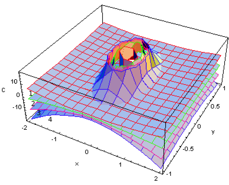
Figure 1: The zero velocity curves (1):$M_{b}=0$, (2):$M_{b}=0.2$,(3):$M_{b}=0.4$, (4):$M_{b}=0.6$, when $\mu=0.025,r=0.8,T=0.01,A_{2}=0,q=1$

The energy integral of the problem is given by $C=2\Omega-{\dot{x}}^{2}-{\dot{y}}^{2}$, where the quantity $C$ is the Jacobi’s constant. The zero velocity curves[see figure ( 1)] are given by:

$$C=2\Omega(x,y)$$ (10)

3 Position of Equilibrium Points

The position equilibrium points of Chermnykh’s probelm is given by putting $\Omega_{x}=\Omega_{y}=0$ i.e.,

$$n^{2}x-\frac{(1-\mu)q_{1}(x+\mu)}{r^{3}_{1}}-\frac{\mu(x+\mu-1)}{r^{3}_{2}}$$

$$-\frac{3}{2}\frac{\mu{A_{2}}(x+\mu-1)}{r^{5}_{2}}-\frac{M_{b}x}{\left(r^{2}+T^{2}\right)^{3/2}}=0,$$ (11)

$$n^{2}y-\frac{(1-\mu)q_{1}{y}}{r^{3}_{1}}-\frac{\mu{y}}{r^{3}_{2}}-\frac{3}{2}\frac{\mu{A_{2}}y}{r^{5}_{2}}$$

$$-\frac{M_{b}y}{\left(r^{2}+T^{2}\right)^{3/2}}=0$$ (12)

From equation ( 12) $n^{2}-\frac{(1-\mu)q_{1}}{r^{3}_{1}}-\frac{\mu}{r^{3}_{2}}-\frac{3}{2}\frac{\mu{A_{2}}}{r^{5}_{2}}-\frac{M_{b}}{\left(r^{2}+T^{2}\right)^{3/2}}=0$ or $y=0$.

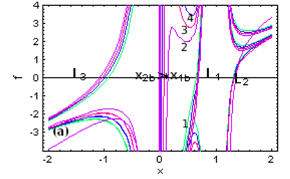
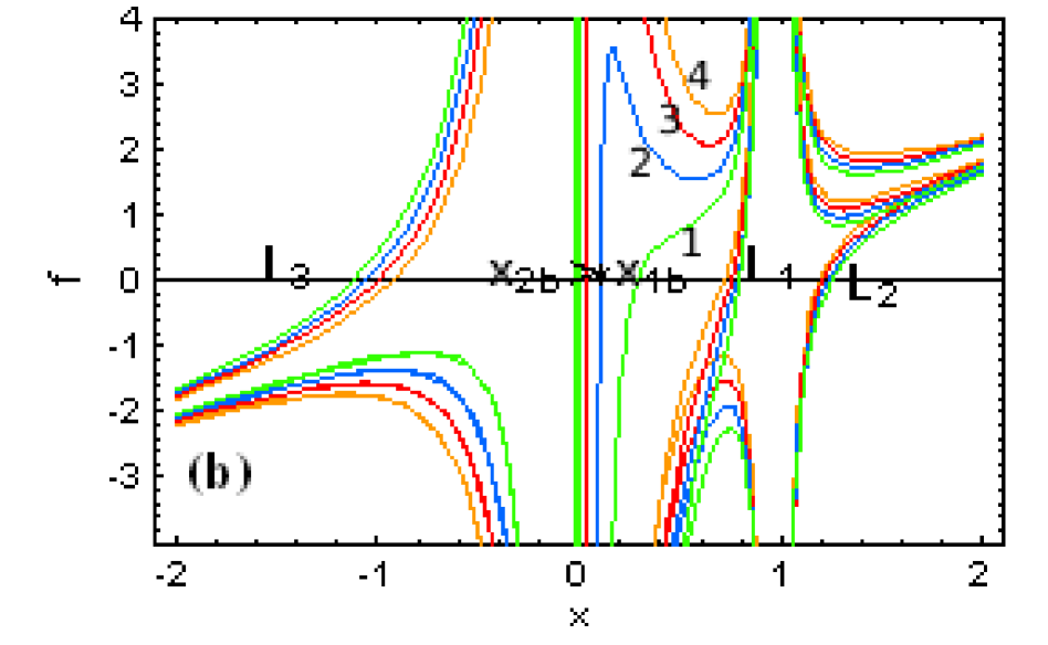
Figure 2: Figure show the position of the collinear equilibrium points in frame (a) when $q_{1}=1,A_{2}=0$ and frame (b) when $q_{1}=1,A_{2}=0.02$, the curves are leveled by (1-4) correspond to the mass of belt $M_{b}=0,0.2,0.4,0.6$.

3.1 Collinear Equilibrium Points

In this case suppose

$$f(x,y)=n^{2}x-\frac{(1-\mu)q_{1}(x+\mu)}{r^{3}_{1}}-\frac{\mu(x+\mu-1)}{r^{3}_{2}}$$

$$-\frac{3}{2}\frac{\mu{A_{2}}(x+\mu-1)}{r^{5}_{2}}-\frac{M_{b}x}{\left(r^{2}+T^{2}\right)^{3/2}}=0,,$$ (13)

$$g(x,y)=\Biggl{[}n^{2}-\frac{(1-\mu)q_{1}}{r^{3}_{1}}-\frac{\mu}{r^{3}_{2}}-\frac{3}{2}\frac{\mu{A_{2}}}{r^{5}_{2}}$$

$$-\frac{M_{b}}{\left(r^{2}+T^{2}\right)^{3/2}}\Biggr{]}y=0$$ (14)

$$f(x,0)=P(x)+Q(x)$$ (15)

where

$$P(x)=n^{2}x-\frac{(1-\mu)q_{1}(x+\mu)}{|x+\mu|^{3}}-\frac{\mu(x+\mu-1)}{|x+\mu-1|^{3}}$$

$$-\frac{3}{2}\frac{\mu{A_{2}}(x+\mu-1)}{|x+\mu-1|^{5}}$$ (16)

$$Q(x)=-\frac{M_{b}x}{\left(x^{2}+T^{2}\right)^{3/2}}=0,$$ (17)

To investigate the position of collinear equilibrium points divide the orbital plane $Oxy$ into three parts with respect to the primaries $x\leq-\mu$, $1-\mu\leq x$ and $-\mu<x<1-\mu$, for each part the function $P(x)$ is defind as follows:

$$P(x)=\begin{cases}n^{2}x+\frac{(1-\mu)q_{1}}{(x+\mu)^{2}}+\frac{\mu}{(x+\mu-1)^{2}}\\ \ +\frac{3}{2}\frac{\mu{A_{2}}}{(x+\mu-1)^{4}}&\text{If}\ x<-\mu,\\ \ n^{2}x-\frac{(1-\mu)q_{1}}{(x+\mu)^{2}}-\frac{\mu}{(x+\mu-1)^{2}}\\ -\frac{3}{2}\frac{\mu{A_{2}}}{(x+\mu-1)^{4}}&\text{If}\ 1-\mu<x,\\ n^{2}x-\frac{(1-\mu)q_{1}}{(x+\mu)^{2}}+\frac{\mu}{|x+\mu-1|^{3}}\\ +\frac{3}{2}\frac{\mu{A_{2}}}{(x+\mu-1)^{4}}&\text{If}\ -\mu<x<1-\mu\end{cases}$$ (18)

When $x\in(-\infty,-\mu)$, $\lim_{x\rightarrow-\infty}f(x,y)<0$, $\lim_{x\rightarrow-\mu^{-}}f(x,y)>0$, $P^{\prime}(x)>0,Q^{\prime}(x)<0$ so there is a point $x_{3}$ for which $f(x_{3},0)=0$. If $x\in(1-\mu,\infty)$, $\lim_{x\rightarrow(1-\mu)^{+}}f(x,y)<0$, $\lim_{x\rightarrow\infty}f(x,y)>0$, $P^{\prime}(x)>0,Q^{\prime}(x)>0$ so there is a point $x_{2}$ for which $f(x_{2},0)=0$. Now $x\in(-\mu,1-\mu)$, $\lim_{x\rightarrow 0^{+}}f(x,y)>0$, $\lim_{x\rightarrow(1-\mu)^{-}}f(x,y)>0$ this implies that an even(or zero) number real roots of $f(x,y)$ exists in this range. If $x\in(-\mu,0)$, consider two cases (i) $x\in(-\mu,-\frac{T}{\sqrt{2}})$ and (ii) $x\in(-\frac{T}{\sqrt{2}}),0)$, we obtained $Q(-\frac{T}{\sqrt{2}})+P(-\frac{T}{\sqrt{2}})>0$ i.e. f$(x,0)\neq 0$ so there is no equilibrium point at $x=-\frac{T}{\sqrt{2}}$. If $Q(-\frac{T}{\sqrt{2}})+P(-\frac{T}{\sqrt{2}})>0$, we obtained $\lim_{x\rightarrow 0^{-}}f(x,y)<0$, $\lim_{x\rightarrow-\mu^{+}}f(x,y)<0$ so there exists two new equilibrium points $x_{b1}\in(-\frac{T}{\sqrt{2}},0)$ and $x_{b2}\in(-\mu,-\frac{T}{\sqrt{2}})$ for which $f(x,0)=0$. But $Q(-\frac{T}{\sqrt{2}})+P(-\frac{T}{\sqrt{2}})<0$ the there exists no equilibrium points in $(-\mu,0)$. If $T<\sqrt{2}\mu$ and $Q(-\frac{T}{\sqrt{2}})+P(-\frac{T}{\sqrt{2}})>0$ then we have two new equilibrium points. Hence we have found there are five equilibrium points on the $x$-axis for the given system. The position of above points are presented graphically by frames a, b in figure ( 2) the curves are leveled by (1-4) correspond to the mass of belt $M_{b}=0,0.2,0.4,0.6$.

3.2 Triangular Equilibrium Points

The triangular equilibrium points are given by putting $\Omega_{x}=\Omega_{y}=0$, $y\neq{0}$. Using the method as Kushvah (2008) then from equations ( 7) and ( 8) we obtained:

$$r_{1} =q_{1}^{1/3}\left[1-\frac{A_{2}}{2}\right.$$ (19)

$$\left.+\frac{(1-2r_{c})M_{b}\left(1-\frac{3\mu A_{2}}{2(1-\mu)}\right)}{3\left(r_{c}^{2}+T^{2}\right)^{3/2}}\right],$$

$$r_{2} =1+\frac{\mu(1-2r_{c})M_{b}}{3\left(r_{c}^{2}+T^{2}\right)^{3/2}}$$ (20)

From above, the triangular equilibriumpoints are as:

$$x=-\mu+\frac{q_{1}^{2/3}}{2}\biggl{[}1-\frac{A_{2}}{}$$

$$+\frac{\mu(2r_{c}-1)M_{b}A_{2}}{(1-\mu)\left(r_{c}^{2}+T^{2}\right)^{3/2}}\biggr{]}$$ (21)

$$y=\pm\frac{q_{1}^{2/3}}{2}\biggl{[}\left(4-q_{1}^{2/3}\right)+2\left(q_{1}^{2/3}-2\right)A_{2}$$

$$+\frac{4(2r_{c}-1)M_{b}\left[\left\{\left(q_{1}^{2/3}-3\right)-\frac{3\mu A_{2}\left(q_{1}^{2/3}-3\right)}{2(1-\mu)}\right\}\right]}{3\left(r_{c}^{2}+T^{2}\right)^{3/2}}\biggr{]}^{1/2}$$ (22)

All these results are similar with Szebehely (1967), Ragos and Zafiropoulos (1995), Jiang and Yeh (2006) and others.

4 Linear Stability

To study the linear stability of any equilibrium point change the origin of the coordinate system to its position $(x*,y*)$ by means of $x=x*+\alpha$,  $y=y*+\beta$, where $\alpha=\xi e^{\lambda{t}}$, $\beta=\eta e^{\lambda{t}}$ are the small displacements $\xi,\eta$,  $\lambda$ these parameters, have to be determined. Therefore the equations of perturbed motion corresponding to the system of equations ( 7), ( 8) may be written as follows:

$$\ddot{\alpha}-2n\dot{\beta} ={\alpha}{\Omega^{*}_{xx}}+{\beta}{\Omega^{*}_{xy}}$$ (23)

$$\ddot{\beta}+2n\dot{\alpha} ={\alpha}{\Omega^{*}_{yx}}+{\beta}{\Omega^{*}_{yy}}$$ (24)

where superfix $*$ is corresponding to the equilibrium points.

$$(\lambda^{2}-{\Omega^{*}_{xx}})\xi+(-2n\lambda-{\Omega^{*}_{xy}})\eta =0$$ (25)

$$(2n\lambda-{\Omega^{*}_{yx}})\xi+(\lambda^{2}-{\Omega^{*}_{yy}})\eta =0$$ (26)

Now above system has singular solution if,

$$\begin{vmatrix}\lambda^{2}-\Omega^{*}_{xx}&-2n\lambda-\Omega^{*}_{xy}\\ 2n\lambda-\Omega^{*}_{yx}&\lambda^{2}-\Omega^{*}_{yy}\\ \end{vmatrix}=0$$

$$\Rightarrow\quad\lambda^{4}+b\lambda^{2}+d=0$$ (27)

At the equilibrium points equations ( 1),( 2) gives us the following:

$$b=2n^{2}-f_{*}-\frac{3\mu{A_{2}}}{{r^{5}_{2}}_{*}}+\frac{3M_{b}T^{2}}{\left(r^{2}_{*}+T^{2}\right)^{5/2}}$$

$$d=9\mu{(1-\mu)}{y^{2}_{*}}\left[\frac{q_{1}}{r^{5}_{1*}r^{5}_{2*}}\right.$$

$$\left.+\frac{3M_{b}}{\left(r^{2}_{*}+T^{2}\right)^{5/2}}\left\{\frac{\mu q_{1}}{{r_{1}^{5}}_{*}}+\frac{(1-\mu){\Bigl{(}1+\frac{5A_{2}}{2{r^{2}_{2}}_{*}}\Bigr{)}}}{r_{2*}^{5}}\right\}\right]$$

where $f_{*}=\frac{(1-\mu)q_{1}}{r^{3}_{1_{*}}}+\frac{\mu}{r^{3}_{2*}}\left(1+\frac{3}{2}\frac{A_{2}}{r^{2}_{2*}}\right)+\frac{3M_{b}}{\left(r^{2}_{*}+T^{2}\right)^{5/2}}$.

The points $L_{1},L_{2},L_{3}$, $x_{b1},x_{b2}$ lie along the line joining the primaries, from ( 19) we have $r_{1}\approx\frac{q_{1}^{1/3}}{n^{2}}$. In this case

$$f = \frac{(1-\mu)q_{1}}{|x+\mu|^{3}}+\frac{\mu}{|x+\mu-1|^{3}}\left(1+\frac{3}{2}\frac{A_{2}}{|x+\mu-1|^{2}}\right)$$ (28)

$$+\frac{3M_{b}}{\left(x^{2}+T^{2}\right)^{5/2}}$$

With the help of equation ( 28) we have drawn figure  3, the different curves (1)-(4) correspond to $M_{b}=0.0,0.2,0.4,0.6$. From this figure we observe that for each $L_{1},L_{2},L_{3}$, $x_{b1}$ and $x_{b2}$, $f>1$, in this case characteristic equation ( 27) has at least one positive root, this implies that collinear equilibrium points are unstable in the sense of Lyapunov.

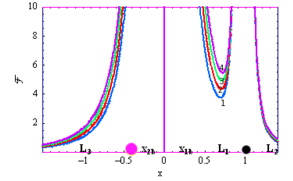
Figure 3: $x-f$, curves correspond to (1):$M_{b}=0$, (2):$M_{b}=0.2$,(3):$M_{b}=0.4$, (4):$M_{b}=0.6$, when $\mu=0.025,r=0.8,T=0.01$, $A_{2}=0$ and $q_{1}=1$

Now we have to study the linear stability of triangular equilibrium points, in this regard we obtained $f=n^{2},\ b=9\mu{(1-\mu)}g$, where $g={y^{2}_{*}}\left[\frac{q_{1}}{r^{5}_{1*}r^{5}_{2*}}\right.\\ \left.+\frac{3M_{b}}{\left(r^{2}_{*}+T^{2}\right)^{5/2}}\left\{\frac{\mu q_{1}}{{r_{1}^{5}}_{*}}+\frac{(1-\mu){\Bigl{(}1+\frac{5A_{2}}{2{r^{2}_{2}}_{*}}\Bigr{)}}}{r_{2*}^{5}}\right\}\right]$. From characteristic equation ( 27) we obtained:

$$\lambda^{2}=\frac{-b\pm{(b^{2}-4d)}^{1/2}}{2}$$ (29)

For stable motion $0<4d<b^{2}$, i.e.

$${\bigl{(}n^{2}-3\mu{A_{2}}\bigr{)}^{2}}>36\mu{(1-\mu)}g$$

In classical case $A_{2}=0,M_{b}=0$, $q_{1}=1$, $n=1$, we have following: $1>27\mu{(1-\mu)}\ \Rightarrow\quad\mu<0.0385201.$ Using equation ( 29) we obtained imaginary roots $\lambda_{1,2}=\pm\mathbf{i}\omega_{1}$, $\lambda_{3,4}=\pm\mathbf{i}\omega_{2}$, $\mathbf{i}=\sqrt{-1}$. The characteristic frequencies $\omega_{1,2}(0<\omega_{2}<\omega_{1})$ are presented by frames (a)-(d) of ( 4– 7) in parameter plots $\omega_{i}-q_{1}$ for different values of $A_{2},q_{1},M_{b}$. They are given in table( 1). We observe that they are decreasing function of radiation pressure and increasing functions of $A_{2},M_{b}$. Hence the triangular equilibrium points are stable in the sense of Lyapunov stability provided $\mu<\mu_{Routh}=0.0385201$.

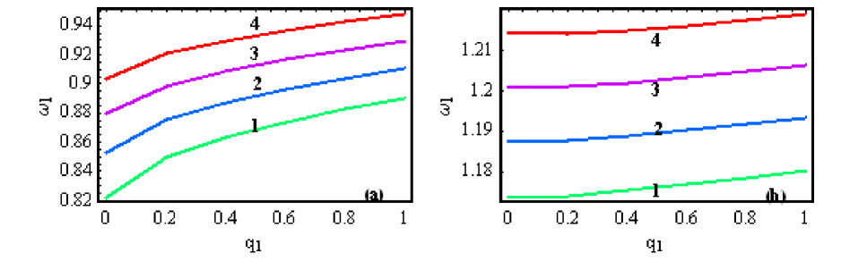
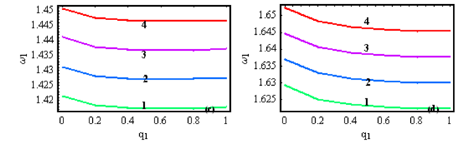
Figure 4: $\omega_{1}-q_{1}$,frames correspond to (a):$M_{b}=0$, (b):$M_{b}=0.2$,(c):$M_{b}=0.4$, (d):$M_{b}=0.6$, curves $(1):A_{2}=0$, $(2):A_{2}=0.02$, $(3):A_{2}=0.04$, $(4):A_{2}=0.06$, $\mu=0.025,r=0.8,T=0.01$

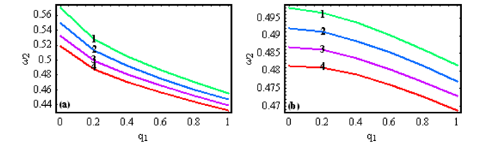
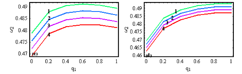
Figure 5: $\omega_{2}-q_{1}$, frames correspond to (a):$M_{b}=0$, (b):$M_{b}=0.2$,(c):$M_{b}=0.4$, (d):$M_{b}=0.6$, curves $(1):A_{2}=0$, $(2):A_{2}=0.02$, $(3):A_{2}=0.04$, $(4):A_{2}=0.06$, $\mu=0.025,r=0.8,T=0.01$

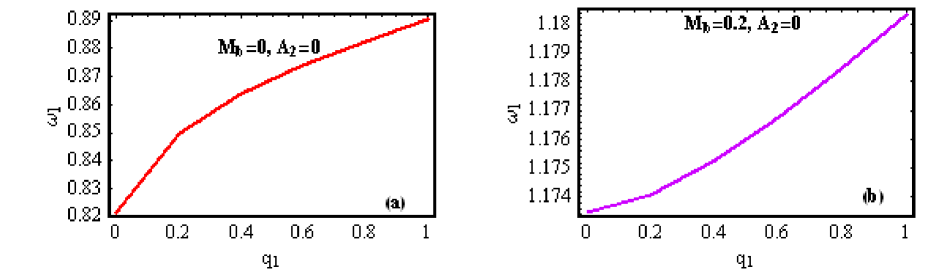
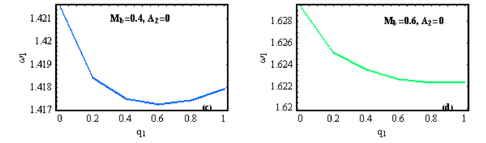
Figure 6: $\omega_{1}-q_{1}$ frames (a):$M_{b}=0$, (b):$M_{b}=0.2$,(c):$M_{b}=0.4$, (d):$M_{b}=0.6$, when $\mu=0.025,r=0.8,T=0.01$

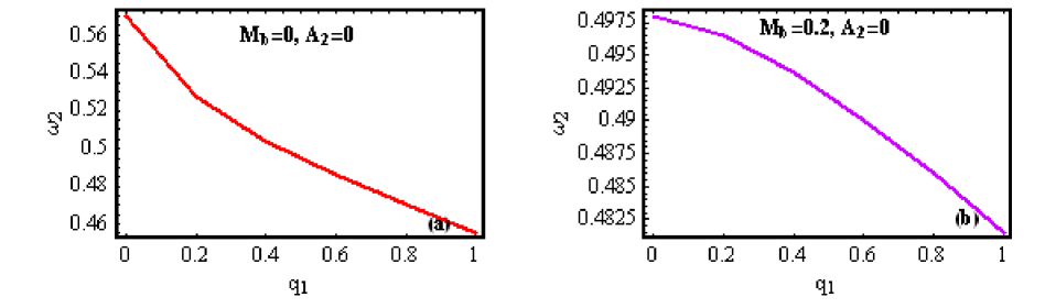
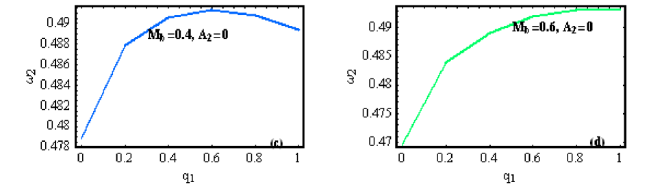
Figure 7: $\omega_{2}-q_{1}$, frames (a):$M_{b}=0$, (b):$M_{b}=0.2$,(c):$M_{b}=0.4$, (d):$M_{b}=0.6$, when $\mu=0.025,r=0.8,T=0.01$

In this case we obtained the three main cases of resonances:

$$\omega_{1}-k\omega_{2}=0,\quad k=1,2,3$$ (30)

For $k=1$ we have positive stable resonance and for $k=2,3$ we have unstable resonances. Using ( 29) and ( 30) we obtained a root of mass parameter:

$$\mu_{k}=\frac{3g+2Kb_{1}b_{2}-\sqrt{g}\sqrt{9g-4Kb_{1}^{2}+12b_{1}b_{2}}}{6(g+Kb_{2}^{2})}$$ (31)

where $K=\frac{k^{2}}{(k^{2}+1)^{2}}$, $b_{1}=n^{2}+\frac{2rM_{b}}{\left(r^{2}+T^{2}\right)^{3/2}}+\frac{3M_{b}T^{2}}{\left(r^{2}+T^{2}\right)^{5/2}}$, $b_{2}=A_{2}\left[1+\frac{5(2r-1)M_{b}}{\left(r^{2}+T^{2}\right)^{3/2}}\right]$. Now we suppose $q_{1}=1-\epsilon$, with $|\epsilon|<<1$, neglecting higher order terms, we obtained the critical mass parameter values corresponding to $k=1,2,3$ as :

$$\mu_{1} = 0.0385208965+0.0375419787A_{2}$$ (32)

$$-0.0089174706\epsilon-0.0678734040M_{b}$$

$$\mu_{2} = 0.0242938971+0.0254350205A_{2}$$ (33)

$$-0.0055364958\epsilon-0.0421398438M_{b}$$

$$\mu_{3} = 0.0135160160+0.0148764140A_{2}$$ (34)

$$-0.0030452832\epsilon-0.0231785159M_{b}$$

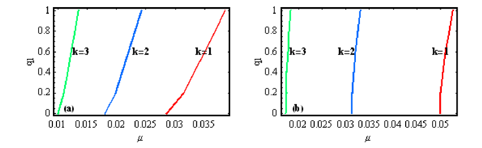
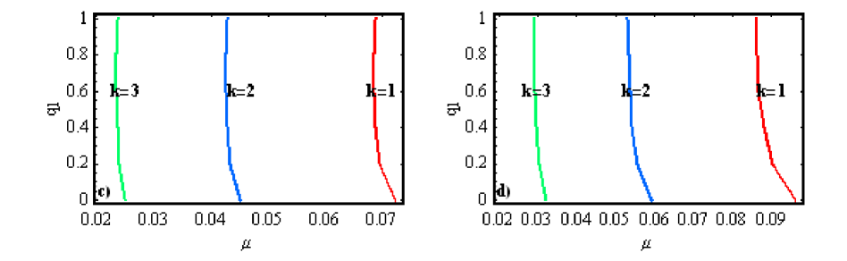
Figure 8: $\mu-q_{1}$ frames correspond to (a):$M_{b}=0$, (b):$M_{b}=0.2$,(c):$M_{b}=0.4$, (d):$M_{b}=0.6$, when $A_{2}=0,k=1-3$, $r=0.8,T=0.01$

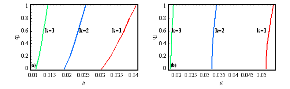
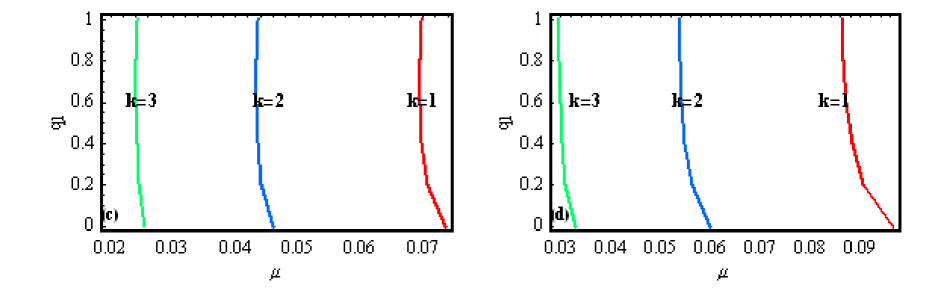
Figure 9: $\mu-q_{1}$ frames correspond to (a):$M_{b}=0$, (b):$M_{b}=0.2$,(c):$M_{b}=0.4$, (d):$M_{b}=0.6$, when $A_{2}=0.02,k=1-3$, $r=0.8,T=0.01$

The linear stability region and main resonance curves $k=1,2,3$ are shown by $\mu-q_{1}$ parameter space frames (a)-(d) in figures ( 8, 9). The curve corresponding to $k=1,(q_{1}=1,A_{2}=0,M_{b}=0,\mu_{1}=\mu_{Routh}=0.038521)$ is actual boundary of the stability region. The critical values of mass parameter $\mu_{k}$ are presented in table ( 2) for various values of $q_{1},A_{2},M_{b}$. The classical critical values of $\mu$ are similar to Deprit and Deprit-Bartholome (1967). These results are similar to the results of Markellos, Papadakis, and Perdios (1996), Kushvah (2008) and others. We observe that the effect of radiation pressure reduces the linear stability zones and the $\mu_{k}$ is an increasing function of $M_{b}$, $A_{2}$.

5 Conclusion

The points $L_{1},L_{2},L_{3}$, $x_{b1},x_{b2}$ lie along the line joining the primaries. We observe that the effect of radiation pressure reduces the linear stability zones, these are also affected by belt and the oblateness of second primary. The collinear equilibrium points are unstable while triangular equilibrium points are stable in the sense of Lyapunov stability provided $\mu<\mu_{Routh}=0.0385201$.

Acknowledgements I am very thankful to Dr. Uday Dolas, Dr. Deepak Singh for their persuasion. I am also thankful to Mrs. Snehlata Kushwah for her loving support. I am grateful to IUCAA Pune for financial assistance to visit library and computer facilities.

Table 1: $\omega_{1,2}$ when $r=0.8,T=0.01,\mu=0.025$

$A_{2}$	$q_{1}$	$\omega_{1}:M_{b}=0$	$\omega_{2}:M_{b}=0$	$\omega_{1}:M_{b}=0.2$	$\omega_{2}:M_{b}=0.2$	$\omega_{1}:M_{b}=0.4$	$\omega_{2}:M_{b}=0.4$	$\omega_{1}:M_{b}=0.6$	$\omega_{2}:M_{b}=0.6$
0.0	1.0	0.890141	0.455686	1.18033	0.4815237	1.41795	0.489382	1.62232	0.493127
	0.75	0.880622	0.47382	1.17804	0.487083	1.41737	0.491041	1.62238	0.492928
	0.5	0.869076	0.494679	1.17602	0.491953	1.41733	0.491159	1.62304	0.490779
	0.25	0.853749	0.520684	1.17436	0.495895	1.41812	0.488893	1.62461	0.485532
	0.0	0.821584	0.570088	1.17349	0.497955	1.4215	0.478958	1.62926	0.4697
0.02	1.0	0.910283	0.447086	1.1934	0.477057	1.42768	0.486598	1.63005	0.491211
	0.75	0.901845	0.463871	1.19127	0.482336	1.42716	0.48813	1.63013	0.490934
	0.5	0.891743	0.483005	1.18941	0.486917	1.42716	0.488124	1.6308	0.488709
	0.25	0.878605	0.506511	1.18791	0.490552	1.42798	0.485737	1.63238	0.48339
	0.0	0.852388	0.549485	1.18724	1.43137	1.43137	0.475658	1.63701	0.467476
0.04	1.0	0.929538	0.439272	1.20624	0.472778	1.43732	0.483883	1.63772	0.489328
	0.75	0.921985	0.45491	1.20426	0.477788	1.43685	0.48529	1.63783	0.488972
	0.5	0.913034	0.47262	1.20254	0.482095	1.43689	0.485164	1.63851	0.486674
	0.25	0.901559	0.494157	1.2012	0.485439	1.43774	0.482658	1.6401	0.481283
	0.0	0.879387	0.532615	1.2007	0.486672	1.44113	0.472436	1.64471	0.465288

 

Note. — Table 1 presents the roots of characteristic equation( 27).

Table 2: $\mu_{k}(A_{2},M_{b})$, when $r=0.8,T=0.01$

$q_{1}$	$k$	$\mu_{k}(0,0)$	$\mu_{k}(0,0.02)$	$\mu_{k}(0,0.4)$	$\mu_{k}(0,0.6)$	$\mu_{k}(0.02,0)$	$\mu_{k}(0.02,0.2)$	$\mu_{k}(0.02,0.4)$	$\mu_{k}(0.02,0.6)$
1.0	1	0.0385209	0.0525812	0.0688051	0.0861218	0.0404877	0.0539744	0.0696964	0.0863953
	2	0.0242939	0.0329695	0.0428408	0.0532015	0.0255597	0.0339343	0.0435889	0.0537117
	3	0.013516	0.0182676	0.0236236	0.0291855	0.0142309	0.0188392	0.0241121	0.0295953
	4	0.00827037	0.0111565	0.014396	0.0177443	0.00871096	0.0115163	0.0147154	0.01803
	5	0.0055092	0.00742441	0.00956953	0.0117815	0.0058038	0.00766762	0.00978937	0.0119837
0.75	1	0.0363201	0.051579	0.0684542	0.0863238	0.0382382	0.0529886	0.0693753	0.0866222
	2	0.0229262	0.0323547	0.0426289	0.0533212	0.024159	0.0333263	0.0433931	0.0538481
	3	0.0127632	0.0179323	0.0235093	0.0292495	0.0134588	0.0113141	0.0240058	0.0296688
	4	0.0078121	0.0109532	0.014327	0.0177827	0.00824062	0.0113141	0.014651	0.0180743
	5	0.00520474	0.00728962	0.00952388	0.0118069	0.00549121	0.0075334	0.00974673	0.012013
0.5	1	0.0341355	0.0507482	0.0685365	0.0872546	0.0359977	0.0521785	0.0694903	0.0875708
	2	0.0215661	0.0318447	0.0426786	0.0538727	0.0227616	0.0328263	0.0434633	0.054418
	3	0.0120136	0.0176539	0.0235361	0.0295437	0.0126877	0.0182322	0.0240439	0.0299757
	4	0.00735548	0.0107843	0.0143431	0.0179594	0.00777057	0.0111476	0.0146741	0.0182594
	5	0.00490128	0.00717768	0.00953459	0.0119234	0.00517872	0.00742292	0.00976201	0.0121354

 

Note. — Table 2 is presents the roots of characteristic equation( 27)

References

- Beletsky and Rodnikov (2008) Beletsky VV, Rodnikov AV (2008) Stability of triangle libration points in generalized restricted circular three-body problem. Cosmic Research 46:40–48, 10.1007/s10604-008-1006-2
- Chermnykh (1987) Chermnykh SV (1987) Stability of libration points in a gravitational field. Leningradskii Universitet Vestnik Matematika Mekhanika Astronomiia pp 73–77
- Das et al (2008) Das MK, Narang P, Mahajan S, Yuasa M (2008) Effect of radiation on the stability of equilibrium points in the binary stellar systems: RW-Monocerotis, Krüger 60. Ap&SS314:261–274, 10.1007/s10509-008-9765-z
- Deprit and Deprit-Bartholome (1967) Deprit A, Deprit-Bartholome A (1967) Stability of the triangular Lagrangian points. AJ72:173