Characteristics of the eigenvalue distribution of the Dirac operator in dense two-color QCD

Abstract:

We exposit the eigenvalue distribution of the lattice Dirac operator in Quantum Chromodynamics with two colors (i.e. two-color QCD). We explicitly calculate all the eigenvalues in the presence of finite quark chemical potential $\mu$ for a given gauge configuration on the finite-volume lattice. First, we elaborate the Banks-Casher relations in the complex plane extended for the diquark condensate as well as the chiral condensate to relate the eigenvalue spectral density to the physical observable. Next, we evaluate the condensates and clarify the characteristic spectral change corresponding to the phase transition. Assuming the strong coupling limit, we exhibit the numerical results for a random gauge configuration in two-color QCD implemented by the staggered fermion formalism and confirm that our results agree well with the known estimate quantitatively. We then exploit our method in the case of the Wilson fermion formalism with two flavors. Also we elucidate the possibility of the Aoki (parity-flavor broken) phase and conclude from the point of view of the spectral density that the artificial pion condensation is not induced by the density effect in strong-coupling two-color QCD.

1 Introduction

Quantum Chromodynamics with two colors (two-color QCD) instead of three is a sophisticated practice ground for theorists to extract worthwhile information out of dense quark matter. We immediately hit on several reasons why we can believe so: First of all, numerous works on dense two-color QCD have almost established a firm understanding on the ground state of two-color QCD by the analytical approach as well as the Monte-Carlo simulation [1, 2, 3, 4, 5, 6, 7, 8, 9, 10, 11, 12, 13, 14, 15, 16, 17, 18, 19, 20, 21, 22, 23, 24, 25, 26, 27, 28, 29, 30, 31]. Second, the notorious sign problem of the Dirac determinant at $\mu\neq 0$ (where $\mu$ is the quark chemical potential) is not so harmful as genuine QCD, which makes it viable to perform the Monte-Carlo integration [1, 11, 25, 32]. Third, dense two-color matter realizes a bosonic baryon system leading to the Bose-Einstein condensation of the color-singlet diquark [6, 7]. This two-color superfluid phase is reminiscent of the three-color superconducting phase [33], for they both break the $\mathrm{U_{B}}(1)$ symmetry. Finally, enlarged flavor symmetry earned by the pseudo-real nature of the SU(2) group that is called Pauli-Gürsey symmetry [35, 34] constrains two-color QCD at $m_{q}=\mu=0$. The interplay between the chiral and diquark sectors simplifies owing to the symmetry, which enables us to construct an effective model for two-color QCD with less ambiguity [21, 25].

This paper aims to illustrate the spectral behavior in a rather brute-forth manner. We usually define the order parameter and concern its expectation value to examine the phase structure with varying the external parameters such as the temperature $T$, the quark chemical potential $\mu$, the quark mass $m_{q}$, and so on. We shall explore our another trail here leading to the phase distinction. In this work we will carefully look into the eigenvalue distribution of the Dirac operator and characterize the state of matter by the distribution pattern. Actually, we can find the scatter plot for the Dirac eigenvalues in two-color QCD in Refs. [4, 11] and we will do that in a more systematic way. It is long known that the eigenvalue spectrum is informative in the vacuum [36] and the random matrix theory is capable of determining the low-lying spectrum, which has recently been extended to the finite density study [29, 31, 37]. Interestingly, the comparison to the random matrix model exhibits good agreement also in the case of the overlap fermion at $\mu\neq 0$ [38].

It is not only the low-lying spectrum but also the whole spectral density that we will deal with in the present paper. The Monte-Carlo simulation generates a set of gauge field configurations each of which has a substantial weight on the partition function. One configuration corresponds to one value for a certain operator (the order parameter for example of our interest), and the more configurations we accumulate, the more accurately we can improve the expectation value of the order parameter. Here, we would remind that the well-known Banks-Casher relation [39] yields the chiral condensate given in terms of the eigenvalue spectral density at the origin (i.e. $m_{q}\to 0$). It follows in turn that the order parameter makes use of only tiny amount of the entire information available from the spectrum. In this work, hence, we will unveil detailed information in a special case of dense and cold ($T=0$) quark matter with two colors.

One might come across a question then; what is the benefit from the whole shape of the eigenvalue distribution? To answer this, we should be aware that the Dirac eigenvalues originally lie on the imaginary axis except for the displacement in the real direction by $m_{q}$ but they scatter over the complex plane because of non-zero chemical potential $\mu\neq 0$ or Wilson coefficient $r\neq 0$. This feature has, more or less, something to do with the sign problem meaning that the Dirac determinant could take a negative value. For $\mu\neq 0$ the Dirac operator mixes the Hermitean and anti-Hermitean operators up resulting in a complex eigenvalue. The situation at finite $\mu$ looks similar to that in the presence of the Wilson term in view of the eigenvalues particularly in the two-color case [32]. [We implicitly assume only the two-color case below.] The sign problem may arise actually when the eigenvalue distribution protrudes from the positive quadrant into the negative quadrant. This observation implies that a large $m_{q}$ (center location of the eigenvalue distribution) as compared to the chemical potential or the Wilson term (distribution width) would put the sign problem away. In the physics language, the vacuum stays empty as long as $m_{q}>\mu$, and so there is no $\mu$ dependence then, which brings about no sign problem naturally. The onset of the density effect is manifestly visible from the whole eigenvalue distribution. Besides, since $m_{q}\neq 0$ shifts the distribution, it is transparent to take account of the mass effect provided that the eigenvalue distribution is given. These motivate us to turn to the entire Dirac spectrum. In the future, hopefully, we believe that the eigenvalue distribution should shed light upon the sign problem at a deeper level. In fact, as we will recognize later, a large value of $\mu$ induces a peculiar structure in the eigenvalue pattern.

The above mentioned may well be somewhat abstract. Let us then make the issue to be discussed more specific. What puzzles us is that there seems to be no clear distinction between the onset criterion for the superfluid phase and the Aoki phase if considered based on the eigenvalue distribution alone. They can possibly coexist but it would be a weird situation because the superfluid phase is a physical ground state but the Aoki phase is a lattice artifact inherent in the Wilson fermion formalism [40, 41]. The final part of this paper will be devoted to resolving this matter. There, we will find that the onset criterion is certainly degenerate when $\mu=0$, but the Aoki phase is taken over by the superfluid state in the proper limit of $\mu\to 0$. In short, we conclude that the Aoki phase never emerges by the density effect in strong-coupling two-color QCD.  This statement does not conflict the preceding strong coupling analysis [40, 41] because the Aoki phase solution at strong coupling is a saddle-point and infinite $N_{\text{c}}$ is required for stability, though this fact is sometimes overlooked.

2 Two-Color QCD at Strong Coupling

In the limit of the strong coupling the gauge action does not enter the dynamics and the partition function is simply given by the fermionic part;

$$Z=\Bigl{\langle}(\det\mathcal{D})^{N_{\text{f}}}\Bigr{\rangle}_{U}\equiv\int\prod_{n,\mu}\mathrm{d}U_{\mu}(n)\,\bigl{(}\det\mathcal{D}\bigr{)}^{N_{\text{f}}}.$$ (1)

Here $\mathcal{D}$ is the Dirac operator. Although the strong coupling limit is a drastic approximation which neglects the gauge dynamics completely, it is amazing that only the Dirac determinant with random gluon fields can grasp rich contents of quark matter not only in the two-color case  [2, 5, 20] but also in the general case [3, 40, 41, 42, 43, 44, 45, 46, 47, 48, 49].

In a box with volume $V=L^{4}$, the operator $\mathcal{D}$ is a $(4N_{\text{c}}V)\times(4N_{\text{c}}V)$ matrix. We denote the eigenvalue of $\mathcal{D}$ by $\lambda_{i}$, that is,

$$\mathcal{D}v_{i}=\lambda_{i}v_{i}\,,$$ (2)

where $i$ runs from $1$ to $4N_{\text{c}}V$. Then the Dirac determinant is given by the product of all the eigenvalues. It is easy to prove that $\det\mathcal{D}$ in the SU(2) gauge theory takes a real value even at finite density where $\mathcal{D}$ loses the $\gamma_{5}$-Hermiticity, i.e. $\gamma_{5}\mathcal{D}(\mu)\gamma_{5}=\mathcal{D}^{\dagger}(-\mu)\neq\mathcal{D}^{\dagger}(\mu)$. The standard argument immediately follows;

$$\det\mathcal{D}(\mu)=\det\bigl{[}(C\sigma_{2}\gamma_{5})^{-1}\mathcal{D}(\mu)(C\sigma_{2}\gamma_{5})\bigr{]}=\det\mathcal{D}^{\ast}(\mu)=\bigl{[}\det\mathcal{D}(\mu)\bigr{]}^{\ast}\,.$$ (3)

Here, to derive the above, the necessary relations we use are $\gamma_{5}\gamma_{\mu}\gamma_{5}=-\gamma_{\mu}$, $C\gamma_{\mu}C^{-1}=-\gamma^{T}_{\mu}$, and $\sigma_{2}U\sigma_{2}=U^{\ast}$ where the last relation corresponds to the pseudo-real nature of the SU(2) group.

From this argument we see that $\det\mathcal{D}(\mu)$ is real but not necessarily positive. The simulation thus entails an even number of $N_{\text{f}}$ so that $(\det\mathcal{D})^{N_{\text{f}}}$ is positive definite. This is the main reason why the exotic phase structure proposed in Refs. [12, 25] in two-color QCD with quark and isospin chemical potentials has been far from confirmed. The two-color determinant, however, buries a nice property of respective eigenvalues under the product. We can prove that, if $\lambda_{i}=m_{q}+\mathrm{i}\lambda_{i}^{\prime}$ is an eigenvalue of the Dirac determinant in two-color QCD, there appear $m_{q}-\mathrm{i}\lambda_{i}^{\prime}$, $m_{q}+\mathrm{i}\lambda_{i}^{\prime\ast}$, and $m_{q}-\mathrm{i}\lambda_{i}^{\prime\ast}$ simultaneously in the eigenvalue spectrum [11, 25, 32]. The proof may break down when $\mathrm{i}\lambda_{i}^{\prime}$ is a real number; the eigenvectors for $m_{q}+\mathrm{i}\lambda_{i}^{\prime}$ and $m_{q}-\mathrm{i}\lambda_{i}^{\prime\ast}$ could not be independent. According to Ref. [11] the staggered fermion is safe from such a possibility but the Wilson fermion has only a pair of $m_{q}+\mathrm{i}\lambda_{i}^{\prime}$ and $m_{q}-\mathrm{i}\lambda_{i}^{\prime}$ instead of a complex quartet in that case of real $\mathrm{i}\lambda_{i}^{\prime}$. We will explicitly verify that this is the case. Then the single-flavor Wilson fermion suffers the sign problem once either of real $m_{q}+\mathrm{i}\lambda_{i}^{\prime}$ and $m_{q}-\mathrm{i}\lambda_{i}^{\prime}$ is negative.

Here we shall briefly summarize the known facts in two-color QCD at strong coupling. Let us begin with the chiral limit. It has been discovered first in Ref. [2] that the chiral condensate is zero, while the diquark condensate has a finite expectation value, in the limit of $\mu\to 0$ with $m_{q}=0$ taken first. In the presence of $m_{q}\neq 0$ the system is kept intact as long as $\mu$ is sufficiently small and, in turn, the chiral condensate becomes non-zero but the diquark condensate vanishes. As soon as $\mu$ exceeds the mass of the lightest excitation (usually bosonic baryon), the density effect is activated leading to decreasing chiral condensate and increasing diquark condensate as $\mu$ goes larger. We remark that this behavior of dense two-color QCD has been settled in the staggered fermion but the relation between the chiral and diquark condensates is not quite convincing yet in the Wilson fermion because the Wilson term breaks chiral symmetry explicitly.

3 Banks-Casher Relations

Here we will make a quick view over the link between the eigenvalue spectral density and the chiral, diquark, and parity-flavor breaking condensates for later usage. In this section the argument holds regardless of strong coupling or not.

3.1 Chiral Condensate

It is widely known that the chiral condensate has a close connection to the Dirac eigenvalue distribution via the Banks-Casher relation [39]. To advance our discussions in a self-contained manner we shall take a brief look at the derivation of the Banks-Casher relation. In the explicit presence of the source for the chiral condensate (i.e. mass term), the Dirac operator could be decomposed into the form of $\mathcal{D}[m]=m_{q}{\rm 1\rule{0.43057pt}{6.54443pt}\hskip 0.86108pt}+\mathcal{D}[0]$ whose eigenvalue is denoted as $\lambda_{i}=m_{q}+\mathrm{i}\lambda_{i}^{\prime}$ as we did in the previous section. The chiral condensate per flavor is given by the derivative of $Z$ with respect to $m_{q}$, which leads us to

$$\begin{split}\frac{1}{N_{\text{f}}}\langle\bar{\psi}\psi\rangle&=-\frac{1}{N_{\text{f}}V}\frac{\partial}{\partial m}\ln Z=-\frac{1}{V}\Bigl{\langle}\sum_{i}\frac{1}{\lambda_{i}}\prod_{j}\lambda_{j}\Bigr{\rangle}_{U}\cdot\Bigl{\langle}\prod_{j}\lambda_{j}\Bigr{\rangle}_{U}^{-1}\equiv\\ &\equiv-\frac{1}{V}\biggl{\langle}\!\!\biggl{\langle}\sum_{i}\frac{1}{\lambda_{i}}\biggr{\rangle}\!\!\biggr{\rangle}=\biggl{\langle}\!\!\biggl{\langle}\oint\frac{\mathrm{d}\lambda}{2\pi\mathrm{i}}\,\frac{\pi\rho_{\chi}(\lambda)}{\lambda}\biggr{\rangle}\!\!\biggr{\rangle}\,,\end{split}$$ (4)

where $\rho_{\chi}(\lambda)$ is the eigenvalue spectral density which is to be expressed in the complex plane as

$$\rho_{\chi}(\lambda)\equiv\frac{1}{\pi V}\sum_{i}\frac{1}{\lambda_{i}-\lambda}\,,$$ (5)

which is, strictly speaking, the resolvent [37] rather than the spectral density. To keep the analogy to the conventional Banks-Casher relation, however, we shall refer to the above as the spectral density. The integration contour should go around all of the poles at $\lambda_{i}$ to pick all the eigenvalues up. In our notation $\langle\cdots\rangle_{U}$ means the ensemble average over gauge configurations and $\langle\!\langle\cdots\rangle\!\rangle$ represents the average including the Dirac determinant.

Here we consider the contour which is an infinitely large circle in the complex plane surrounding all the poles. Then the contour integral must amount to zero because $\rho_{\chi}(\lambda)/\lambda$ goes to zero faster than $|\lambda|^{-1}$. That means that we can evaluate the above integral by the negative residue of the pole at $\lambda=0$. After all, we have

$$\langle\bar{\psi}\psi\rangle=-N_{\text{f}}\,\pi\bigl{\langle}\!\bigl{\langle}\rho_{\chi}(0)\bigr{\rangle}\!\bigr{\rangle}\,.$$ (6)

For consistency check let us consider a bit more about this formula. Usually the Banks-Casher relation is given in the limit of $m_{q}\to 0$. In this limit, using the notation $\lambda_{i}=m_{q}+\mathrm{i}\lambda_{i}^{\prime}$ where $\lambda_{i}^{\prime}$ is a real number in the continuum theory, we can rewrite Eq. (5) into a form of

$$\rho_{\chi}(0)=\lim_{m_{q}\to 0}\frac{1}{\pi V}\sum_{i}\frac{1}{m_{q}+\mathrm{i}\lambda_{i}^{\prime}}=\frac{1}{V}\sum_{i}\delta(\lambda_{i}^{\prime})\,,$$ (7)

which is more familiar in literatures. We note that Eq. (5) is in fact an analytic continued form of the expression (7) with the delta function, and it is equivalent to the definition of the resolvent used in the context of the random matrix theory [29]. This complex extension is necessary for our purpose since the Dirac operator loses Hermiticity at finite density or in the Wilson fermion formalism. One might have noticed that the Banks-Casher relation in the complex plane is a trivial relation; it is obvious from Eq. (5) that $-\pi\rho_{\chi}(0)$ returns to $\sum_{i}\lambda_{i}^{-1}$ immediately.

3.2 Diquark Condensate

We can develop the same argument for the diquark condensate as well as the chiral condensate. We shall limit our discussions to the case with degenerate two-flavor ($u$ and $d$) quarks, and then we do not need to introduce the Nambu-Gor’kov basis. In the presence of the same quark chemical potential $\mu$ for $u$ and $d$ quarks, we can write the Lagrangian density down as [23]

$$\mathcal{L}=\bar{\psi}_{u}\mathcal{D}(\mu)\psi_{u}+\bar{\psi}_{d}\mathcal{D}(\mu)\psi_{d}-J\bar{\psi}_{u}(C\gamma_{5})\sigma_{2}\bar{\psi}_{d}^{T}+\bar{J}\psi_{d}^{T}(C\gamma_{5})\sigma_{2}\psi_{u}\,,$$ (8)

where $J$ and $\bar{J}$ are the source for the diquark and anti-diquark which are anti-symmetric in spin, color, and flavor. By means of a variable change by

$$\bar{\phi}_{d}\equiv\psi_{d}^{T}C\sigma_{2}\,,\quad\phi_{d}\equiv C\sigma_{2}\bar{\psi}_{d}^{T}\,,$$ (9)

it is possible to compactify the above into

$$\mathcal{L}=(\bar{\psi}_{u},\bar{\phi}_{d})\begin{pmatrix}\mathcal{D}(\mu)\;&-J\gamma_{5}\\ \bar{J}\gamma_{5}\;\;&\mathcal{D}(-\mu)\end{pmatrix}\begin{pmatrix}\psi_{u}\\ \phi_{d}\end{pmatrix}\,.$$ (10)

The integration over the quark fields is then straightforward and the resultant partition function is given as the determinant as follows;

$$Z(J)=\Biggl{\langle}\det\begin{pmatrix}\mathcal{D}(\mu)\gamma_{5}&-J\\ \bar{J}&\mathcal{D}(-\mu)\gamma_{5}\end{pmatrix}\Biggr{\rangle}_{U}=\Bigl{\langle}\det\Bigl{[}\mathcal{D}(\mu)\mathcal{D}^{\dagger}(\mu)+|J|^{2}\Bigr{]}\Bigr{\rangle}_{U}\,,$$ (11)

where we have used $\gamma_{5}\mathcal{D}(-\mu)\gamma_{5}=\mathcal{D}^{\dagger}(\mu)$. We note that $\mathcal{D}(\mu)\mathcal{D}^{\dagger}(\mu)$ is always Hermitean though $\mathcal{D}(\mu)$ may not be so. We can then prove that the eigenvalue of $\mathcal{D}(\mu)\mathcal{D}^{\dagger}(\mu)$ is non-negative real, which we denote by $\xi_{i}^{2}$ with choosing $\xi_{i}\geq 0$. The diquark condensate thus reads

$$\bigl{\langle}\bar{\psi}_{u}(C\gamma_{5})\sigma_{2}\bar{\psi}^{T}_{d}\bigr{\rangle}=\frac{\partial}{V\partial J}Z(J)\Bigr{|}_{J=0}=\frac{1}{V}\biggl{\langle}\!\!\biggl{\langle}\sum_{i}\frac{J}{\xi_{i}^{2}+|J|^{2}}\biggr{\rangle}\!\!\biggr{\rangle}=\pi\bigl{\langle}\!\bigl{\langle}\rho_{D}(0)\bigr{\rangle}\!\bigr{\rangle}\,,$$ (12)

where we have defined the diquark spectral density,

$$\rho_{D}(\xi)=\frac{1}{V}\sum_{i}\delta(\xi-\xi_{i})\,,$$ (13)

in a familiar form. It should be mentioned that we do not have to perform the analytic continuation this time because $\xi_{i}$ sits on the real axis.

3.3 Parity-Flavor Breaking Condensate

In the same way we can discuss the parity-flavor breaking condensate whose non-zero expectation value characterizes the Aoki phase in the Wilson fermion formalism. For two-flavor quarks the source term for the condensate $\langle\bar{\psi}\mathrm{i}\gamma_{5}\tau_{3}\psi\rangle$ enters the Lagrangian as

$$\mathcal{L}=\bar{\psi}_{u}\mathcal{D}(\mu)\psi_{u}+\bar{\psi}_{d}\mathcal{D}(\mu)\psi_{d}+H(\bar{\psi}_{u}\mathrm{i}\gamma_{5}\psi_{u}-\bar{\psi}_{d}\mathrm{i}\gamma_{5}\psi_{d})\,,$$ (14)

from which the partition function reads

$$Z(H)=\Biggl{\langle}\det\begin{pmatrix}\mathcal{D}(\mu)\gamma_{5}+\mathrm{i}H&0\\ 0&\mathcal{D}(\mu)\gamma_{5}-\mathrm{i}H\end{pmatrix}\Biggr{\rangle}_{U}=\Bigl{\langle}\det\Bigl{[}\mathcal{D}(\mu)\mathcal{D}^{\dagger}(-\mu)+H^{2}\Bigr{]}\Bigr{\rangle}_{U}\,.$$ (15)

It is interesting to note that Eq. (15) above is reduced to Eq. (11) when $\mu=0$. As a result the parity-flavor breaking condensate seems to be degenerate with the diquark condensate in the absence of chemical potential. Once the finite density is switched on, $D(\mu)D^{\dagger}(-\mu)$ is no longer a Hermitean operator, and its eigenvalue distribution spreads over the complex plane. Thus, if we define the spectral density by

$$\rho_{H}(\eta)\equiv\frac{1}{\pi V}\sum_{i}\frac{1}{\eta_{i}-\eta}$$ (16)

with the complex eigenvalue $\eta_{i}^{2}$ of the operator $\mathcal{D}(\mu)\mathcal{D}^{\dagger}(-\mu)$ with choosing $\text{Re}(\eta_{i})\geq 0$, we can write the parity-flavor breaking condensate as

$$\bigl{\langle}\bar{\psi}_{u}\mathrm{i}\gamma_{5}\psi_{u}-\bar{\psi}_{d}\mathrm{i}\gamma_{5}\psi_{d}\bigr{\rangle}=-\mathrm{i}\pi\bigl{\langle}\!\bigl{\langle}\rho_{H}(\mathrm{i}H)-\rho_{H}(-\mathrm{i}H)\bigr{\rangle}\!\bigr{\rangle}=2\pi\text{Im}\bigl{\langle}\!\bigl{\langle}\rho_{H}(\mathrm{i}H)\bigr{\rangle}\!\bigr{\rangle}\,.$$ (17)

4 Eigenvalue Distribution for a Random Configuration

In this work we will take only one random configuration as a representative instead of calculating the ensemble average over many random configurations. Actually the eigenvalue distribution for one typical gauge configuration turns out to be quite informative in our case. This simplification is legitimate because each random configuration equally contributes to a physical quantity in the strong coupling limit. So to speak, the strong coupling theory is democratic and any configuration is eligible for a representative. If we are interested in the weak coupling regime, we would have to take an appropriate ensemble average.

We will first proceed to the calculation in the staggered fermion formalism and make sure that our results agree well with known results in the mean-field approximation at strong coupling. After that we will adopt the Wilson fermion formalism and look further into the possibility of the Aoki phase.

4.1 Staggered Fermion

The Dirac operator at finite density in the staggered fermion formalism is

$$\begin{split}\mathcal{D}_{S}(\mu)&\equiv m_{q}\,\delta_{m,n}+\frac{1}{2}\sum_{i}\eta_{i}(m)\Bigl{[}U_{i}(m)\,\delta_{m+\hat{\imath},n}-U^{\dagger}_{i}(n)\,\delta_{m,n+\hat{\imath}}\Bigr{]}+\\ &\quad+\eta_{4}(m)\Bigl{[}\mathrm{e}^{\mu}\,U_{4}(m)\,\delta_{m+\hat{4},n}-\mathrm{e}^{-\mu}\,U^{\dagger}_{4}(n)\,\delta_{m,n+\hat{4}}\Bigr{]}\,,\end{split}$$ (18)

where $\eta_{\mu}(n)\equiv(-1)^{n_{1}+n_{2}+\cdots+n_{\mu-1}}$ and the chemical potential is introduced as formulated in Ref. [50].

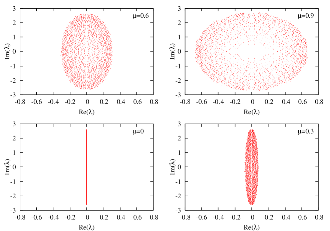
Figure 1: Eigenvalue distribution for a random gauge configuration in the staggered fermion formalism at $m_{q}=0$ on the $6^{4}$ lattice. The distribution at $m_{q}\neq 0$ is given by a shift along the real axis by $m_{q}$.

The zero-density Dirac operator in the staggered fermion formalism is anti-Hermitean except for the mass term, so that all the eigenvalues reside on the vertical line whose real part is $m_{q}$ (see the lower-left scatter plot in Fig. 1). The chemical potential breaks Hermiticity and the eigenvalue distribution has a width along the real axis as $\mu$ goes larger as shown in the scatter plots for $\mu=0.3$, $0.6$, and $0.9$ in Fig. 1. These figures are reminiscent of the scatter plots in Refs. [4, 11]. To draw Fig. 1 we have generated a random gauge configuration on the lattice with a volume of $V=6^{4}$. Because the staggered fermion has only color indices, the total number of dots in Fig. 1 is $2\times 6^{4}=2592$ for each plot. We have made use of LAPACK to compute $2592$ eigenvalues numerically.

The broadened width in the real direction has a definite physical meaning. In the case of $m_{q}\neq 0$ the distribution has to be shifted by $m_{q}$ and then the entire eigenvalue distribution can be placed in the positive quadrant as long as $\mu$ is small as compared to $m_{q}$. It is hence a natural anticipation that the superfluidity has an onset when the eigenvalue distribution becomes as wide as it reaches the origin. This is actually the case.

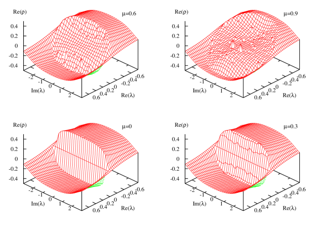
Figure 2: Real part of the spectral density, $\text{Re}(\rho_{\chi}(\lambda))$, in the complex plane for various values of the chemical potential.

From the obtained eigenvalues we can explicitly calculate the spectral density (5) to evaluate the chiral condensate through the Banks-Casher relation in Eq. (6). Because of the quartet pattern of the eigenvalue distribution the imaginary part of $\rho_{\chi}(\lambda)$ is vanishing on the real axis. The chiral condensate inferred from Eq. (6) is thus insensitive to the imaginary part but determined solely by the real part of the spectral density taking a real value. We show the real part of the spectral density (5) in Fig. 2 for various $\mu$. It is remarkable that the spectral density for a random configuration looks such smooth even without taking an ensemble average.

As we have mentioned, the eigenvalues and thus the spectral density with a finite $m_{q}$ can be deduced simply by a shift along the real axis by $m_{q}$. Therefore, $\rho_{\chi}(0)$ appearing in Eq. (6) can be read from Fig. 2 by the value at $(\text{Re}\lambda,\text{Im}\lambda)=(-m_{q},0)$.

When $\mu=0$ a sharp perpendicular wall stands at $\text{Re}(\lambda)=0$ which is responsible for a non-vanishing chiral condensate in the limit of $m_{q}\to 0$ while keeping $\mu=0$. The wall is smoothened by the effect of $\mu\neq 0$ and it is no longer vertically upright at finite density, which leads to an interesting observation. In fact, it is not hard to conceive from Fig. 2 that the chiral condensate becomes zero in the chiral limit at infinitesimal but nonzero $\mu$. This is absolutely consistent with Ref. [2].

We shall next evaluate the diquark condensate using the Banks-Casher relation (12). We will start with the chiral limit ($m_{q}=0$) and then go into the finite mass case that we choose $m_{q}=0.2$ here in this work. For convenience we define the integrated diquark spectral number,

$$n_{D}(\xi)=\int_{0}^{\xi}\!\mathrm{d}\xi^{\prime}\,\rho_{D}(\xi^{\prime})\,,$$ (19)

whose slope at $\xi=0$ gives the spectral density $\rho_{D}(\xi=0)$ which is proportional to the diquark condensate. Although the staggered fermion Lagrangian does not involve the Dirac spinor, it is not difficult to make use of the Nambu-Gor’kov representation to express the diquark condensate by the diquark spectral density. Since the derivation is only straightforward, we will not reiterate it but skip detailed arithmetics. To summarize the resultant relations, we can prove that

$$\sigma\equiv\frac{1}{2}\langle\bar{\chi}\chi\rangle=\frac{\pi}{2}\rho(0)\,,\qquad\Delta\equiv\frac{1}{2}\langle\chi\mathrm{i}\sigma_{2}\chi\rangle=\frac{\pi}{4}\rho_{D}(0)\,,$$ (20)

where the extra $1/2$ factor in the diquark relation comes from the square-root prescription necessary to cancel the doubled Nambu-Gor’kov basis. In the above we have chosen the same normalization as Ref. [20].

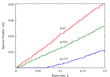
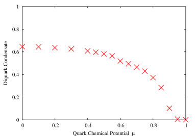
Figure 3: Left) Histogram of $n_{D}(\xi)$ whose slope gives the spectral density $\rho_{D}(\xi)$. Right) Diquark condensate as a function of $\mu$ at $m_{q}=0$.

It is intriguing to evaluate $n_{D}(\xi)$ by the explicit numerical calculation for the eigenvalues in Fig. 2 from which we can get $\rho_{D}(\xi)$. Figure 3 shows our results in the chiral limit. In this case only the diquark condensate is a non-vanishing quantity [2]. We plot the diquark condensate in the right of Fig. 3 without indicating the error bar. We did so because, though the fitting error is small, the systematic error is large. If we change the working procedure to measure the slope from the histogram in the left of Fig. 3, the resultant diquark condensate would change too. For clarity of our numerical procedure we explain how we compute the slope of $n_{D}(\xi)$ at the origin. We assume a functional form $n_{D}(\xi)=a\xi+b\xi^{2}$ within the range $\xi\in[0,0.1]$ and fix $a$ and $b$ to fit the data. Then, $a$ gives the slope at the origin. If $a$ turns negative, that means no spectral density at the origin, and so the diquark condensate should be zero. In this way we draw the right of Fig. 3 which shows outstanding agreement with the upper-left of Fig. 1 in Ref. [20].

The $m_{q}$ dependence in $\mathcal{D}(\mu)\mathcal{D}^{\dagger}(\mu)$ is not such trivial as in the case of $\mathcal{D}(\mu)$. Roughly speaking, a finite $m_{q}$ shifts the eigenvalue in the positive real direction so that the eigenvalue distribution is blocked in the vicinity of the origin as long as $\mu$ is small. For $\mu$ above a certain threshold value the diquark spectral density becomes finite at $\xi=0$, and the diquark condensation is activated. We can repeat the calculation in the massive case as well. As we mentioned our choice is $m_{q}=0.2$, and we read the chiral and diquark condensate from the chiral and diquark spectral density. Our final results are presented below in Fig. 4. We note that the onset for the chiral condensate decrease is determined by the front edge of the sidling wall which corresponds to the edge of the Dirac eigenvalue distribution, which in turn corresponds to the diquark onset.

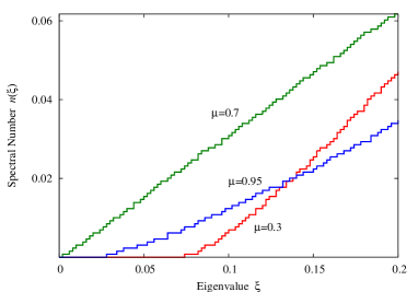
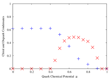
Figure 4: Left) Histogram of $n_{D}(\xi)$ in the case of $m_{q}=0.2$. Right) Chiral and diquark condensates as a function of $\mu$ at $m_{q}=0.2$.

It is impressing that the results in the right of Fig. 4 is consistent qualitatively with the mean-field analysis in the strong coupling limit given in the upper-left of Fig. 1 in Ref. [20], though the direct comparison is not possible for different mass choice.

4.2 Wilson Fermion

We shall consider the Wilson fermion henceforth. The Dirac operator is defined as

$$\begin{split}\mathcal{D}_{W}(\mu)&\equiv\delta_{m,n}-\kappa\sum_{i}\Bigl{[}(r-\gamma_{i})\,U_{i}(m)\,\delta_{m+\hat{\imath},n}+(r+\gamma_{i})\,U^{\dagger}_{i}(n)\,\delta_{m,n+\hat{\imath}}\Bigr{]}-\\ &\quad-\kappa\Bigl{[}(r-\gamma_{4})\,\mathrm{e}^{\mu}\,U_{4}(m)\,\delta_{m+\hat{\imath},n}+(r+\gamma_{4})\,\mathrm{e}^{-\mu}\,U^{\dagger}_{4}(n)\,\delta_{m,n+\hat{\imath}}\Bigr{]}\,,\end{split}$$ (21)

where $\kappa$ is the hopping parameter and we choose $r=1$ throughout this work. In this case we adopt $V=4^{4}$ and then there are (2 colors)$\times$(4 spinors)$\times 4^{4}=2048$ eigenvalues. Of course, we could treat $V=6^{4}$ without difficulty, but there are then many eigenvalues (almost five times more than the $V=4^{4}$ case) and plotting looks too dense. Our small lattice volume is limited not for technical reason but for presentation convenience.

It is instructive to see the free dispersion relations first. With the free background (i.e. $U_{\mu}={\rm 1\rule{0.43057pt}{6.54443pt}\hskip 0.86108pt}$ everywhere) it is easy to calculate the eigenvalue analytically in momentum space to find

$$\begin{split}\text{Re}(\lambda_{\text{free}})&=1-2\kappa r\bigl{(}\cos p_{1}+\cos p_{2}+\cos p_{3}+\cos p_{4}\bigr{)}\,,\\ \text{Im}(\lambda_{\text{free}})&=\pm 2\kappa\sqrt{(\sin p_{1})^{2}+(\sin p_{2})^{2}+(\sin p_{3})^{2}+(\sin p_{4})^{2}}\,.\end{split}$$ (22)

Although this expression is valid only for the free background, it turns out to be quite useful to understand the eigenvalue distribution in a qualitative level even at strong coupling as we will see shortly.

Usually $\text{Re}(\lambda)<0$ gives the condition that the Aoki phase appears. In the free case, therefore, the Aoki phase has a window $|\kappa|>1/(8r)$, while the Aoki phase condition is $|\kappa|>1/(4r)$ in the strong coupling limit. Now, as we mentioned in Introduction, it is confusing that the diquark condensation has exactly the same criterion for the onset, as demonstrated in Figs. 1 and 2. Then, a question arises; which of the diquark superfluid phase and the Aoki phase is more favored? The rest of this paper will be devoted to answering this question.

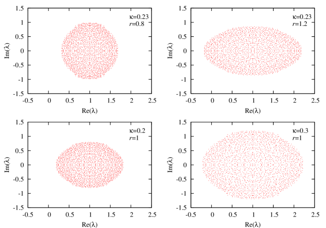
Figure 5: Eigenvalue distribution for a random gauge configuration in the Wilson fermion formalism at $\mu=0$ on the $4^{4}$ lattice for various combinations of $\kappa$ and $r$.

Let us see the parameter dependence of the eigenvalue distribution for a random configuration in the zero density case, which is shown in Fig. 5. When we increase $\kappa$ with $r$ fixed as shown in the lower two figures in Fig. 5, the distribution range is enlarged. We can understand this qualitatively from Eq. (22) in the free dispersion; both $\text{Re}(\lambda)-1$ and $\text{Im}(\lambda)$ are proportional to $\kappa$. The upper two plots in Fig. 5 show the $r$ dependence with $\kappa$ fixed. In this case in turn the distribution stretches only along the real axis. This feature is also manifest in Eq. (22) since only $\text{Re}(\lambda)-1$ is multiplied by $r$. As we can see, the distribution penetrates into the negative real region between $(r=1,\kappa=0.2)$ and $(r=1,\kappa=0.3)$, which is consistent with the known fact that the critical coupling is $(r=1,\kappa=0.25)$ in the strong coupling limit. In what follows we will employ a value of $\kappa=0.23$ which is close to the critical point but still outside of the Aoki phase region, if any.

Next, we will investigate how the chemical potential affects the eigenvalue distribution. Let us consider the free case first again in which the fourth component is replaced as $p_{4}\to p_{4}-\mathrm{i}\mu$. Then, the real and imaginary parts in the free dispersion are, respectively, modified by

$$\begin{split}\cos(p_{4}-\mathrm{i}\mu)&=\cosh\mu\cos p_{4}+\mathrm{i}\sinh\mu\sin p_{4}\,,\\ \bigl{[}\sin(p_{4}-\mathrm{i}\mu)\bigr{]}^{2}&=(\sin p_{4})^{2}-(\sinh\mu)^{2}-{\textstyle\frac{1}{2}}\mathrm{i}\sinh(2\mu)\sin(2p_{4})\,.\end{split}$$ (23)

In this simple case it is interesting to see how the free known results are affected by the effect of the finite chemical potential which we show in Fig. 6.

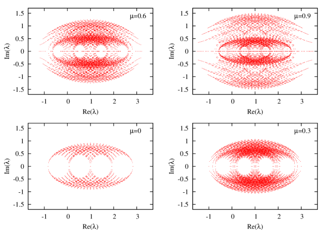
Figure 6: Eigenvalue distribution for the free Wilson fermion at $\kappa=0.23$ on the $4^{4}$ lattice for $\mu=0$, $0.3$, $0.6$, and $0.9$.

To draw Fig. 6 we have discretized the momenta $p_{1}$, $p_{2}$, $p_{3}$, and $p_{4}$ in the range $[-\pi,\pi]$ into twenty points with equal spacing. We did so in order to make the “density” perceivable from Fig. 6; if the momentum is close to continuum with many points, the distribution except for the $\mu=0$ case does not have the empty region strictly. The concentration would be hard to see. It is quite interesting to observe a non-trivial structure emerging at high $\mu$ unexpectedly. It is apparent that the density has a similar effect as the hopping parameter $\kappa$; the eigenvalue profile becomes wider in the complex plane as either $\mu$ or $\kappa$ gets greater. The density modification is not such simple, however, and we presume that the rich contents in dense quark matter are attributed in part to this structural difference.

At the same time, however, we have to keep in mind that this complicated structure at large $\mu$ looks like coming from the non-trivial entanglement between different doubler sectors. In the vicinity of the continuum limit at $\mu=0$ only the far left edge part corresponds to the lightest physical excitation and four other points crossing the real axis are doublers going to infinity. This clear separation is missing in view of the eigenvalue distribution of Fig. 6 at $\mu=0.6$ or at $\mu=0.9$ for instance. This poses a serious question; even though we could solve the sign problem somehow, it should be a subtle issue how to separate the doublers out at density high enough to allow for excitations of unphysical doublers.

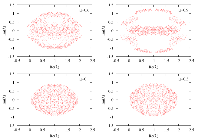
Figure 7: Eigenvalue distribution for a random gauge configuration in the Wilson fermion formalism at $\kappa=0.23$ on the $4^{4}$ lattice for $\mu=0$, $0.3$, $0.6$, and $0.9$.

For a randomly generated gauge configuration the $\mu$ dependence of the eigenvalue distribution reflects the above mentioned structure as displayed in Fig. 7. Needless to say, we can follow the same path to evaluate the chiral condensate but the resulting condensate is finite and almost constant independent of the density. This is because naive chiral symmetry is explicitly broken in the Wilson fermion formalism, and so we will not present the results. Let us now evaluate the diquark condensate in the same way as we did in the staggered fermion formalism. It is calculable from the integrated spectral number $n_{D}(\xi)$ for the operator $\mathcal{D}(\mu)\mathcal{D}^{\dagger}(\mu)$. Our results are shown in Fig. 8.

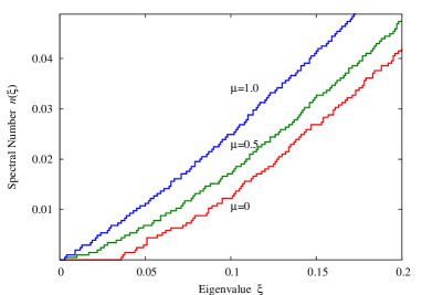
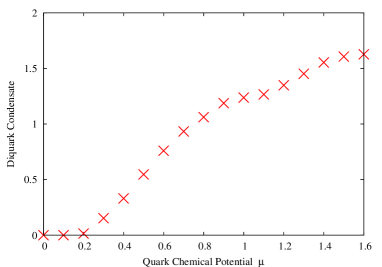
Figure 8: Left) Histogram of $n_{D}(\xi)$. Right) Diquark condensate as a function of $\mu$.

In the case of the Wilson fermion there are four times degrees of freedom than the staggered fermion and so the saturation effect is not yet relevant in the right of Fig. 8. It should be mentioned that we measure the slope at the origin in the same way as in the staggered fermion; we fit the data up to $\xi=0.1$ by $n_{D}(\xi)=a\xi+b\xi^{2}$. If we change the fitting range and the fitting functional form, we would have quantitatively different results. The systematic error is not well under control. At least, however, we can state that such simple calculations in this work could capture qualitative features of diquark superfluidity.

Finally let us discuss the possibility of the Aoki phase from the point of view of the spectral density $\rho_{H}(\eta)$ corresponding to the parity-flavor breaking condensate. That is understood from the 3D plot for the spectral density given in Fig. 9.

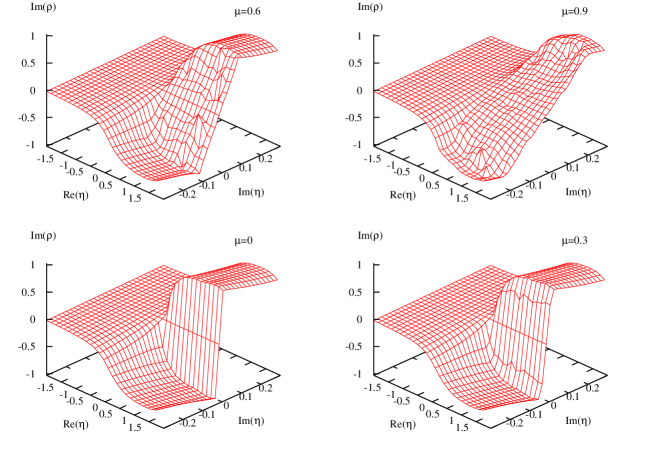
Figure 9: Imaginary part of the spectral density, $\text{Im}(\rho_{H}(\eta))$ in the complex plane for various values of the chemical potential.

According to the Banks-Casher-type relation we obtained, the parity-flavor breaking condensate is to be acquired from the height of $\text{Im}(\rho_{H}(\eta))$ at the origin. It should be the finite-volume effect that the origin looks smooth and the symmetry breaking looks like not occurring even at $\mu=0$. We anticipate that the standing wall would be more sharp upright around the origin in the thermodynamic limit. Even in the thermodynamic limit, however, the wall has a finite slope at $\mu\neq 0$ which reminds us of the chiral condensate discussed in Fig. 2. Thus, the same conclusion can be drawn; the parity-flavor breaking condensate thus takes a non-zero value in the limit of $H\to 0$ while keeping $\mu=0$ strictly. In the presence of infinitesimal chemical potential, in contrast, the situation changes and the condensate is vanishing in the limit of $\mu\to 0$ after taking the limit $H=0$. Therefore, in the exactly same sense as the chiral dynamics we should conclude that there is no parity-flavor breaking condensate in this system. As long as the two-color QCD with two degenerate flavors is concerned, we do not have to care about the Aoki phase even in the Wilson fermion formalism on the lattice.

5 Remarks

We saw the eigenvalue distribution of the Dirac operator at finite density $\mathcal{D}(\mu)$ and its relatives $\mathcal{D}(\mu)\mathcal{D}^{\dagger}(\mu)$ and $\mathcal{D}(\mu)D^{\dagger}(-\mu)$ to discuss the fate of the chiral condensate, the diquark condensate, and the parity-flavor breaking condensate.

We have a conjecture that a similar pattern in the eigenvalue distribution should appear also in dense QCD with three colors; the eigenvalue distribution reaches the origin at the onset for nuclear matter. At this stage we have no idea what kind of characteristic feature is associated with the color superconducting phase. We believe, in principle, that we can pursue our strategy in order to access color superconductivity. It has not been successful so far to describe the color superconducting phase in the strong coupling limit [51]. Since our method does not assume any mean-field nor truncation, our method should be useful to clarify what is going on in the diquark channel in strong-coupling QCD.  This is what we are planning to do as a future extension.

The present work is focused on the numerical outputs. It is maybe an interesting question how the change in the eigenvalue distribution could be interpreted in analogy to known phenomena such as the chiral symmetry breaking interpreted as the Anderson localization [52, 53, 54]. This research deserves further investigation. Also, it should be feasible, in principle, to apply our idea to the weak-coupling regime close to the continuum limit using the open gauge configurations if they are available. Since the physical units in the color SU(2) world are obscure, unfortunately, the continuum limit is not quite lucid then. Nevertheless, in view of the qualitative success of the strong coupling expansion to understand hot and dense QCD [48], we may well anticipate that a smooth crossover links the strong-coupling regime to the weak-coupling one. This could be checked by inclusion of the finite $\beta$ corrections.

Finally let us mention on the possible extension to the overlap fermion where exact chiral symmetry can be defined on the lattice. Then, there is no need to consider the Aoki phase from the beginning because the eigenvalue distribution sits on a single circle line at $\mu=0$. This nice feature breaks down, however, at finite density. This is because the $\gamma_{5}$-hermiticity is lost at $\mu\neq 0$ but it is amazing that chiral symmetry is still realized [38]. The overlap fermion surpasses the staggered and Wilson fermions; we would be able to treat not four but two flavors and look into the behavior of the chiral condensate as well as the diquark condensate in the overlap fermion formalism. This extension is also on our list for future perspective.

- [1] A. Nakamura, Phys. Lett. B 149 (1984) 391.
- [2] E. Dagotto, F. Karsch and A. Moreo, Phys. Lett. B 169 (1986) 421.
- [3] E. Dagotto, A. Moreo and U. Wolff, Phys. Lett. B 186 (1987) 395.
- [4] C. Baillie, K. C. Bowler, P. E. Gibbs, I. M. Barbour and M. Rafique, Phys. Lett. B 197 (1987) 195.
- [5] J. U. Klatke and K. H. Mutter, Nucl. Phys. B 342 (1990) 764.
- [6] R. Rapp, T. Schafer, E. V. Shuryak and M. Velkovsky, Phys. Rev. Lett. 81 (1998) 53 [hep-ph/9711396].
- [7] G. W. Carter and D. Diakonov, Phys. Rev. D 60 (1999) 016004 [hep-ph/9812445].
- [8] S. Hands, J. B. Kogut, M. P. Lombardo and S. E. Morrison, Nucl. Phys. B 558 (1999) 327 [hep-lat/9902034].
- [9] J. B. Kogut, M. A. Stephanov and D. Toublan, Phys. Lett. B 464 (1999) 183 [hep-ph/9906346].
- [10] J. B. Kogut, M. A. Stephanov, D. Toublan, J. J. M. Verbaarschot and A. Zhitnitsky, Nucl. Phys. B 582 (2000) 477 [hep-ph/0001171].
- [11] S. Hands, I. Montvay, S. Morrison, M. Oevers, L. Scorzato and J. Skullerud, Eur. Phys. J. C 17 (2000) 285 [hep-lat/0006018].
- [12] K. Splittorff, D. T. Son and M. A. Stephanov, Phys. Rev. D 64 (2001) 016003 [hep-ph/0012274].
- [13] J. B. Kogut, D. Toublan and D. K. Sinclair, Phys. Lett. B 514 (2001) 77 [hep-lat/0104010].
- [14] J. B. Kogut, D. K. Sinclair, S. J. Hands and S. E. Morrison, Phys. Rev. D 64 (2001) 094505 [hep-lat/0105026].
- [15] J. B. Kogut, D. Toublan and D. K. Sinclair, Nucl. Phys. B 642 (2002) 181 [hep-lat/0205019].
- [16] K. Splittorff, D. Toublan and J. J. M. Verbaarschot, Nucl. Phys. B 639 (2002) 524 [hep-ph/0204076].
- [17] J. Wirstam, J. T. Lenaghan and K. Splittorff, Phys. Rev. D 67 (2003) 034021 [hep-ph/0210447].
- [18] S. Muroya, A. Nakamura and C. Nonaka, Phys. Lett. B 551 (2003) 305 [hep-lat/0211010].
- [19] J. B. Kogut, D. Toublan and D. K. Sinclair, Phys. Rev. D 68 (2003) 054507 [hep-lat/0305003].
- [20] Y. Nishida, K. Fukushima and T. Hatsuda, Phys. Rev. 398 (2004) 281 [hep-ph/0306066].
- [21] C. Ratti and W. Weise, Phys. Rev. D 70 (2004) 054013 [hep-ph/0406159].
- [22] B. Alles, M. D’Elia and M. P. Lombardo, Nucl. Phys. B 752, 124 (2006) [arXiv:hep-lat/0602022].
- [23] S. Hands, S. Kim and J. I. Skullerud, Eur. Phys. J. C 48 (2006) 193 [hep-lat/0604004].
- [24] K. Fukushima and Y. Hidaka, Phys. Rev. D 75 (2007) 036002 [hep-ph/0610323].
- [25] K. Fukushima and K. Iida, Phys. Rev. D 76 (2007) 054004 [\arXivid0705.0792 [hep-ph]].
- [26] M. A. Stephanov, Phys. Rev. Lett. 76 (1996) 4472 [hep-lat/9604003].
- [27] A. M. Halasz, J. C. Osborn and J. J. M. Verbaarschot, Phys. Rev. D 56 (1997) 7059 [hep-lat/9704007].
- [28] B. Vanderheyden and A. D. Jackson, Phys. Rev. D 64 (2001) 074016 [hep-ph/0102064].
- [29] G. Akemann and T. Wettig, Phys. Rev. Lett. 92 (2004) 102002 [Erratum-ibid. 96, 029902 (2006)] [hep-lat/0308003].
- [30] B. Klein, D. Toublan and J. J. M. Verbaarschot, Phys. Rev. D 72 (2005) 015007 [hep-ph/0405180].
- [31] G. Akemann and E. Bittner, Phys. Rev. Lett. 96 (2006) 222002 [hep-lat/0603004].
- [32] K. Fukushima, PoS LATTICE2007, 185 (2007).
- [33] For a recent review; see, M. G. Alford, A. Schmitt, K. Rajagopal and T. Schafer, \arXivid0709.4635 [hep-ph].
- [34] A. Smilga and J. J. M. Verbaarschot, Phys. Rev. D 51 (1995) 829 [hep-th/9404031].
- [35] M. E. Peskin, Nucl. Phys. B 175 (1980) 197.
- [36] R. Setoodeh, C. T. H. Davies and I. M. Barbour, Phys. Lett. B 213 (1988) 195.
- [37] G. Akemann, Int. J. Mod. Phys. A 22 (2007) 1077 [hep-th/0701175].
- [38] J. Bloch and T. Wettig, Phys. Rev. Lett. 97 (2006) 012003 [hep-lat/0604020].
- [39] T. Banks and A. Casher, Nucl. Phys. B 169 (1980) 103.
- [40] S. Aoki, Phys. Rev. D 30 (1984) 2653.
- [41] S. Aoki, Nucl. Phys. B 314 (1989) 79.
- [42] N. Kawamoto and J. Smit, Nucl. Phys. B 192 (1981) 100.
- [43] J. Hoek, N. Kawamoto and J. Smit, Nucl. Phys. B 199 (1982) 495.
- [44] H. Kluberg-Stern, A. Morel and B. Petersson, Nucl. Phys. B 215 (1983) 527.
- [45] H. Kluberg-Stern, A. Morel, O. Napoly and B. Petersson, Nucl. Phys. B 220 (1983) 447.
- [46] K. Fukushima, Phys. Lett. B 553 (2003) 38 [hep-ph/0209311].
- [47] K. Fukushima, Phys. Rev. D 68 (2003) 045004 [hep-ph/0303225].
- [48] K. Fukushima, Prog. Theor. Phys. Suppl. 153 (2004) 204 [hep-ph/0312057].
- [49] N. Kawamoto, K. Miura, A. Ohnishi and T. Ohnuma, Phys. Rev. D 75 (2007) 014502 [hep-lat/0512023].
- [50] P. Hasenfratz and F. Karsch, Phys. Lett. B 125 (1983) 308.
- [51] V. Azcoiti, G. Di Carlo, A. Galante and V. Laliena, J. High Energy Phys. 0309 (2003) 014 [hep-lat/0307019].
- [52] A. M. Garcia-Garcia and J. C. Osborn, Phys. Rev. D 75 (2007) 034503 [hep-lat/0611019].
- [53] T. T. Takahashi, J. High Energy Phys. 0711 (2007) 047 [hep-lat/0703023].
- [54] T. T. Takahashi, J. High Energy Phys. 0805 (2008) 094 [\arXivid0803.2216 [hep-lat]].