Reduction of the gravitational lens equation to a one-dimensional non-linear form for the tilted Plummer model family

Abstract

The gravitational lens equation for the tilted Plummer family of models can be reduced to a one-dimensional non-linear equation. For certain values of the slope of the radial profile it can be reduced to a polynomial form. Both forms are advantageous to find the roots, i.e. the images for a given model. The critical curve equations can also be reduced to a non-linear or polynomial form, and therefore it is useful to find the caustics. This lens model family has ample use in gravitational lens theory, and can produce up to five images.

1 Introduction

Smooth non-singular isothermal sphere (SNIS) models are often used in gravitational lens theory. Including ellipticity, these models are called elliptical SNIS (ESNIS) (Blandford & Kochanek, 1987) or tilted Plummer family (Kassiola & Kovner, 1993). This class of models can be generated from elliptical mass distributions or elliptical potentials. The models obtained by means of mass distributions are realistic even for higher ellipticities. The models generated using the elliptical potentials are restricted to small ellipticities (Kassiola & Kovner, 1993), because the isodensity contours become dumbbell-shaped for higher ellipticities. Moreover, the density for these elliptical potencials could be negative for certain combinations of parameters (Kassiola & Kovner, 1993). For more information about these models, the interested reader may consult the references at the end of this Letter.

For ESNIS models, the gravitational lens equation (GLE) becomes non-linear, and hard to solve if the external perturbations (density and shear) are taken into account. However, for ESNIS models obtained from elliptical potentials, it is possible to simplify this equation to a one-dimensional non-linear or polynomial form. We will show how to do it.

The advantage of reducing the GLE to a one-dimensional non-linear or polynomial form is that there is simple iterative methods to get the roots of this class of equations. The critical curve equation can also be reduced to a non-linear or polynomial form. This allows us to find the caustics easily. Examples of these models will be presented in this Letter.

2 ESNIS Models

The tilted Plummer family of elliptic potentials has the form

$$\psi({\bf x})=\left\{\begin{array}[]{cc}\frac{\kappa_{0}}{2\beta}(x^{2}_{0}+\varepsilon_{1}x^{2}_{1}+\varepsilon_{2}x^{2}_{2})^{\beta}-\psi_{0},&0<\beta<1\\ \frac{\kappa_{0}}{2}\ln{(x^{2}_{0}+\varepsilon_{1}x^{2}_{1}+\varepsilon_{2}x^{2}_{2})},&\beta=0,\end{array}\right.$$ (1)

where ${\bf x}=(x_{1},\,x_{2})$, $x_{1}$ and $x_{2}$ are measured in the direction of the principal axes of the ellipsoid (image position), $\beta$ is the slope of the radial profile of the potential, $x_{0}$ is the core radius (same units as $x_{1}$ and $x_{2}$), $\kappa_{0}$ is a constant, $\varepsilon_{i}=1\pm\varepsilon$ ($i=1,\,2$) with $\varepsilon$ as the lens ellipticity, and $\psi_{0}$ is a constant potential reference, which will be taken as null.

The scaled deflection angle components for the ESNIS models have the following form:

$$\alpha_{i}({\bf x})=\frac{\kappa_{i}x_{i}}{(x^{2}_{0}+\varepsilon_{1}x^{2}_{1}+\varepsilon_{2}x^{2}_{2})^{1-\beta}},$$ (2)

where $\kappa_{i}=\kappa_{0}\varepsilon_{i}$.

The surface mass density is given by

$$\kappa({\bf x})=\kappa_{0}(x^{2}_{0}+\varepsilon_{1}x^{2}_{1}+\varepsilon_{2}x^{2}_{2})^{\beta-2}[x_{0}^{2}+\beta_{1}\varepsilon_{1}x^{2}_{1}+\beta_{2}\varepsilon_{2}x^{2}_{2}],$$

where $\beta_{i}=1+(\beta-1)\varepsilon_{i}$.

To avoid negative values of surface mass density and the dumbbell form of the isodensity contour shape, the ellipticity $\varepsilon$ should be restricted to small values (Kassiola & Kovner, 1993):

$$\varepsilon\leq\frac{\beta}{3-\beta}.$$

Among the models, that the ESNIS class contains are:

• power-law mass ($\varepsilon=0,\,\rm{and}\;x_{0}=0$),

• NIS ($\beta=1/2,\,\rm{and}\;\varepsilon\leq 1/5$),

• Plummer ($\beta=\varepsilon=0$).

3 Reduction to a Non-linear or Polynomial Form

The scaled ray tracing equation, or GLE is (Schneider et al., 1992)

$${\bf y}={\sf M}{\bf x}-{\mn@boldsymbol{\alpha}}({\bf x}),$$ (3)

where ${\bf y}$ is the source position on the source plane, and the matrix ${\sf M}$ is given by

$${\sf M}=\left(\begin{array}[]{cc}1-\sigma-\gamma\cos{2\phi}&-\gamma\sin{2\phi}\\ -\gamma\sin{2\phi}&1-\sigma+\gamma\cos{2\phi}\end{array}\right),$$ (4)

where $\sigma$, and $\gamma$ are the density and shear of external perturbations (nearby galaxies or a cluster contribution), and $\phi$ is the shear angle.

Let us define some variables for the sake of simplicity

$$\chi = x^{2}_{0}+\varepsilon_{1}x^{2}_{1}+\varepsilon_{2}x^{2}_{2},$$ (5)

$$f(\chi) = {\chi}^{1-\beta}\Rightarrow\chi(f)=f^{1/(1-\beta)}.$$

With these definitions the GLE system takes the form

$$y_{1} = \left(M_{11}-\frac{\kappa_{1}}{f}\right)x_{1}+M_{12}x_{2},$$ (6)

$$y_{2} = \left(M_{22}-\frac{\kappa_{2}}{f}\right)x_{2}+M_{21}x_{1}.$$ (7)

Solving for $x_{1}$ and $x_{2}$, we get

$$gx_{1} = \left(M_{22}-\frac{\kappa_{2}}{f}\right)y_{1}-M_{12}y_{2}=:f_{1},$$ (8)

$$gx_{2} = \left(M_{11}-\frac{\kappa_{1}}{f}\right)y_{2}-M_{21}y_{1}=:f_{2},$$ (9)

where

$$g=\left(M_{11}-\frac{\kappa_{1}}{f}\right)\left(M_{22}-\frac{\kappa_{2}}{f}\right)-M_{12}M_{21}.$$ (10)

Substituting (8) and (9) into (5) yields

$$g^{2}\chi(f)=x_{0}^{2}g^{2}+\varepsilon_{1}f_{1}^{2}+\varepsilon_{2}f_{2}^{2}.$$ (11)

By substitution of the right-hand side of equations (8), (9), and (10) into the last equation, we obtain

$$(\chi(f)-x_{0}^{2})P_{1}(f)=P_{2}(f),$$ (12)

where

$$P_{1}(f) = [f^{2}g]^{2}$$

$$= [(M_{11}f-{\kappa_{1}})(M_{22}f-{\kappa_{2}})-M_{12}M_{21}f^{2}]^{2}$$

$$= [{\cal M}f^{2}-(\kappa_{1}M_{22}-\kappa_{2}M_{11})f+\kappa_{1}\kappa_{2}]^{2},$$

and

$$P_{2}(f) = \{\varepsilon_{1}[(M_{22}f-{\kappa_{2}})y_{1}-M_{12}y_{2}f]^{2}$$ (14)

$$+ \varepsilon_{2}[(M_{11}f-{\kappa_{1}})y_{2}-M_{21}y_{1}f]^{2}\}f^{2}$$

$$= (A_{2}f^{2}-A_{1}f+A_{0})f^{2},$$

with

$${\cal M}=\mathrm{det}[{\bf M}]=M_{11}M_{22}-M_{12}M_{21},$$

$$A_{2}=\varepsilon_{1}(M_{22}y_{1}-M_{12}y_{2})^{2}+\varepsilon_{2}(M_{11}y_{2}-M_{21}y_{1})^{2},$$

$$A_{1}=2[\kappa_{2}\varepsilon_{1}y_{1}(M_{22}y_{1}-M_{12}y_{2})+\kappa_{1}\varepsilon_{2}y_{2}(M_{11}y_{2}-M_{21}y_{1})]$$

and

$$A_{0}=\varepsilon_{1}(\kappa_{2}y_{1})^{2}+\varepsilon_{2}(\kappa_{1}y_{2})^{2}.$$

$P_{1}(f)$ and $P_{2}(f)$ are both fourth order polynomials.

From (12) we get

$$f[P_{1}(f)]^{1-\beta}=[P_{2}(f)+x_{0}^{2}P_{1}(f)]^{1-\beta}.$$ (15)

The last equation is a non-linear one-dimensional equation for $f$ that can be solved by means of iterative numerical methods, for example, the Brent method (Moré & Cosnard, 1980).

Now, if we set $\beta=m/n$, with $m,\;n$ integers ($n\geq m$), then (15) becomes a polynomial form:

$$f^{n}[P_{1}(f)]^{n-m}=[P_{2}(f)+x_{0}^{2}P_{1}(f)]^{n-m}.$$ (16)

The image positions can be obtained as follows: first of all solve (15) or (16); now substituting the $f$-values into the equations (8), (9), and (10) yield $f_{1}$, $f_{2}$, and $g$; finally use equations (8) and (9) again to get $x_{1}$ and $x_{2}$.

4 The Critical Curves and Caustics

The critical curve is the curve formed by all image positions on which the determinant of the Jacobian vanishes and the caustic curve is the projection of this critical curve to the source plane.

The components of the Jacobian ${\sf J}=\partial{\bf y}/\partial{\bf x}$ are

$$J_{11}=\frac{\partial y_{1}}{\partial x_{1}} = \left(M_{11}-\frac{\kappa_{1}}{f}\right)+{2(1-\beta)\kappa_{1}\varepsilon_{1}x_{1}^{2}}{\chi^{\eta}},$$

$$J_{12}=\frac{\partial y_{1}}{\partial x_{2}} = M_{12}+{2(1-\beta)\kappa_{1}\varepsilon_{2}x_{1}x_{2}}{\chi^{\eta}},$$

$$J_{21}=\frac{\partial y_{2}}{\partial x_{1}} = M_{21}+{2(1-\beta)\kappa_{2}\varepsilon_{1}x_{1}x_{2}}{\chi^{\eta}},$$ (17)

$$J_{22}=\frac{\partial y_{2}}{\partial x_{2}} = \left(M_{22}-\frac{\kappa_{2}}{f}\right)+{2(1-\beta)\kappa_{2}\varepsilon_{2}x_{2}^{2}}{\chi^{\eta}},$$

where $\eta=\beta-2$.

The determinant of the Jacobian is

$${\cal J} = \mathrm{det}[{\sf J}]=J_{11}J_{22}-J_{12}J_{21}$$

$$= \frac{1}{[fP_{1}(f)]^{2}}\left[\left((M_{11}f-\kappa_{1})P_{1}(f){\phantom{f^{2}}}\right.\right.$$

$$+ \left.\left.{2(1-\beta)\kappa_{1}\varepsilon_{1}}f^{3}[{\cal C}_{1}f-\kappa_{2}y_{1}]^{2}\chi^{\eta}\right)\right.$$

$$\times \left.\left((M_{22}f-\kappa_{2})P_{1}(f){\phantom{f^{2}}}\right.\right.$$

$$+ \left.\left.{2(1-\beta)\kappa_{2}\varepsilon_{2}}f^{3}[{\cal C}_{2}f-\kappa_{1}y_{2}]^{2}\chi^{\eta}\right)\right.$$

$$- \left.\left({2(1-\beta)\kappa_{1}\varepsilon_{2}}({\cal C}_{1}f-\kappa_{2}y_{1})({\cal C}_{2}f-\kappa_{1}y_{2})f^{3}\chi^{\eta}\right.\right.$$

$$- \left.\left.M_{12}fP_{1}(f){\phantom{f^{2}}}\!\!\!\!\!\!\right)\right.$$

$$\times \left.\left({2(1-\beta)\kappa_{2}\varepsilon_{1}}({\cal C}_{1}f-\kappa_{2}y_{1})({\cal C}_{2}f-\kappa_{1}y_{2})f^{3}\chi^{\eta}\right.\right.$$

$$- \left.\left.M_{21}fP_{1}(f){\phantom{f^{2}}}\!\!\!\!\!\!\right)\right],$$

where

$${\cal C}_{1}=M_{22}y_{1}-M_{12}y_{2}$$

and

$${\cal C}_{2}=M_{11}y_{2}-M_{21}y_{1}.$$

In (4) we have substituted (8) and (9). From (4), it is clear that the critical and caustic curves could also be found by solving a one-dimensional non-linear equation or a polynomial in $f$.

5 Examples

5.1 Plummer’s model

Let us take $\beta=0$. We get from (15) the following polynomial:

$$B_{5}f^{5}-B_{4}f^{4}+B_{3}f^{3}+B_{2}f^{2}+B_{1}f-B_{0}=0,$$ (19)

where

$$B_{5}={\cal M}^{2},$$

$$B_{4}={\cal M}^{2}x_{0}^{2}+\varepsilon_{1}{\cal C}_{1}^{2}+\varepsilon_{2}{\cal C}_{2}^{2}+2{\cal C}_{3}{\cal M},$$

$$B_{3}=2\kappa_{1}\kappa_{2}{\cal M}+(2x_{0}^{2}{\cal M}+{\cal C}_{3}){\cal C}_{3}+2\kappa_{2}\varepsilon_{1}y_{1}{\cal C}_{1}+2\kappa_{1}\varepsilon_{2}y_{2}{\cal C}_{2},$$

$$B_{2}=2\kappa_{1}\kappa_{2}{\cal C}_{3}-\kappa_{2}^{2}\varepsilon_{1}y_{1}^{2}-\kappa_{1}^{2}\varepsilon_{2}y_{2}^{2}-x_{0}^{2}[{\cal C}_{3}^{2}+2\kappa_{1}\kappa_{2}{\cal M}],$$

$$B_{1}=\kappa_{1}\kappa_{2}[\kappa_{1}\kappa_{2}-2x_{0}^{2}{\cal C}_{3}]$$

and

$$B_{0}=[x_{0}\kappa_{1}\kappa_{2}]^{2},$$

with

$${\cal C}_{3}=\kappa_{1}M_{22}+\kappa_{2}M_{11}.$$

The Source, images, critical curves, and caustics for this model are shown in Fig. 1. The values of the model parameters are $\sigma=0.05$, $\gamma=0.2$, $\phi=36^{\circ}$, $\varepsilon=0$, $\kappa_{0}=1$ and $x_{0}=0.5$. The critical curves and caustics are inclined, because we have chosen $\phi\neq 0$.

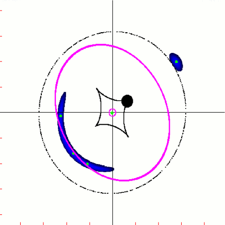
Figure 1: Source (large black dot near the centre), two extended images (one of them is a long blue arc) and one tiny image at the centre (green dot), the critical curves (magenta ellipse and small circle), and the caustics (black diamond and dotted ellipse) produced by the Plummer model for following parameter values $\beta=\varepsilon=0,\;\gamma=0.2,\;\sigma=0.05,\;\phi=36^{\circ},\kappa_{0}=1,\;x_{0}=1/2$. The green dots are the positions of the images for a point source. The position of the extended source is $(0.65,\;0.45)$. The critical curves and caustics are inclined, because $\phi\neq 0$. The window size is $500\times 500$ pixel.

5.2 ESNIS model

Let us take $\beta=1/2$. We also get from (15) a polynomial:

$$B_{6}f^{6}-B_{5}f^{5}+B_{4}f^{4}-B_{3}f^{3}+B_{2}f^{2}+B_{1}f-B_{0}=0,$$ (20)

where

$$B_{6}={\cal M}^{2},$$

$$B_{5}=2{\cal C}_{3}{\cal M}^{2},$$

$$B_{4}={\cal C}_{3}^{2}+2\kappa_{1}\kappa_{2}{\cal M}-[{\cal M}^{2}x_{0}^{2}+\varepsilon_{1}{\cal C}_{1}^{2}+\varepsilon_{2}{\cal C}_{2}^{2}],$$

$$B_{3}=2[{\cal C}_{3}(x_{0}^{2}{\cal M}-\kappa_{1}\kappa_{2})+\kappa_{2}\varepsilon_{1}y_{1}{\cal C}_{1}+\kappa_{1}\varepsilon_{2}y_{2}{\cal C}_{2}],$$

$$B_{2}=[\kappa_{1}\kappa_{2}]^{2}-x_{0}^{2}[2\kappa_{1}\kappa_{2}{\cal M}+{\cal C}_{3}]-\kappa_{2}^{2}\varepsilon_{1}y_{1}^{2}-\kappa_{1}^{2}\varepsilon_{2}y_{2}^{2},$$

$$B_{1}=2\kappa_{1}\kappa_{2}x_{0}^{2}{\cal C}_{3}$$

and

$$B_{0}=[x_{0}\kappa_{1}\kappa_{2}]^{2}.$$

In Fig. 2 the source, images, critical curves, and caustics for this model are shown. The values of the model parameters are $\sigma=\gamma=0.05$, $\phi=36^{\circ}$, $\varepsilon=0.2$, $\kappa_{0}=1$, and $x_{0}=0.5$. The critical curves and caustics are again inclined ($\phi\neq 0$). For this model, one gets up to five images. We have tried with other $\beta$-values (with different values for the other parameters) to find more than five images, but all of our ESNIS models always produce no more than five images.

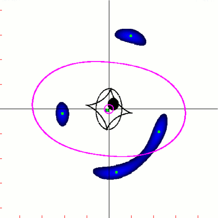
Figure 2: Source (large black dot near the centre), five images (one of them a long blue arc and one small image near the source), the critical curves (magenta ellipse and small circle), and the caustics (black ellipse and diamond) produced by a ESNIS model for following parameter values $\beta=1/2,\;\varepsilon=0.2,\;\gamma=\sigma=0.05,\;\phi=36^{\circ},\kappa_{0}=1,\;x_{0}=1/2$. The green dots are the positions of the images for a point source. The position of the extended source is $(0.2,\;0.2)$. The critical curves and caustics are inclined, because $\phi\neq 0$. The window size is $500\times 500$ pixel.

We have designed XFGLENSES, an interactive program intended to visualize and model gravitational lenses (Frutos-Alfaro, 2001). The modelling part of this program is not finished yet. The Figures 1, and 2 were generated with this software. The interested reader can download it from

http://www.tat.physik.uni-tuebingen.de/~frutto/.

On this Website, there is also extensive information about the software. To solve the GLEs, the Brent method was implemented in the program. To visualize the extended images, we use the Kayser-Schramm method (Schramm & Kayser, 1987; Kayser & Schramm, 1988).

6 Conclusions

Although the ESNIS model generated from elliptical potentials have an ellipticity restriction, these models are very useful in gravitational lens theory. The polynomial reduction presented here is useful not only to invert the GLE, but also to find the critical curves and caustics of a given ESNIS model. Moreover it could be useful to model gravitational lenses with small ellipticities. This class of models always produces up to five images. XFGLENSES can be used to visualize the results of this class of models. To see the capabilities and models that this software has available, visit the Website mentioned above.

7 Acknowledgements

The author would like to thank the German Academic Exchange Service (DAAD: Deutscher Akademischer Austauschdienst) for its financial support and Professor Hans Ruder for the invitation to a research stay in Tübingen.

References

• Blandford & Kochanek (1987) Blandford R.D., Kochanek C.S., 1987, ApJ, 321, 658
• Frutos-Alfaro (2001) Frutos-Alfaro F., 2001, Am. Jour. of Phys., 69, 218
• Kassiola & Kovner (1993) Kassiola K., Kovner I., 1993, ApJ, 417, 450
• Kayser & Schramm (1988) Kayser R., Schramm T., 1988, A & A, 191, 39
• Moré & Cosnard (1980) Moré J.J., Cosnard M.Y., 1980, ACM Trans. on Math. Software, 6, 240
• Schneider et al. (1992) Schneider P., Ehlers J., Falco E., 1992, Gravitational Lenses, Springer, Berlin
• Schramm & Kayser (1987) Schramm T, Kayser R., 1987, A & A, 174, 361