Two-dimensional one-component plasma
on a Flamm’s paraboloid

Abstract

We study the classical non-relativistic two-dimensional one-component plasma at Coulomb coupling $\Gamma=2$ on the Riemannian surface known as Flamm’s paraboloid which is obtained from the spatial part of the Schwarzschild metric. At this special value of the coupling constant, the statistical mechanics of the system are exactly solvable analytically. The Helmholtz free energy asymptotic expansion for the large system has been found. The density of the plasma, in the thermodynamic limit, has been carefully studied in various situations.

Keywords: Coulomb systems, one-component plasma, non constant curvature.

I Introduction

The system under consideration is a classical (non quantum) two-dimensional one-component plasma: a system composed of one species of charged particles living in a two-dimensional surface, immersed in a neutralizing background, and interacting with the Coulomb potential. The one-component classical Coulomb plasma is exactly solvable in one dimension S. F. Edwards and A. Lenard (1962). In two dimensions, in their 1981 work, B. Jancovici and A. Alastuey Jancovici (1981); A. Alastuey and B. Jancovici (1981) showed how the partition function and $n$-body correlation functions of the two-dimensional one-component classical Coulomb plasma (2dOCP) on a plane can be calculated exactly analytically at the special value of the coupling constant $\Gamma=\beta q^{2}=2$, where $\beta$ is the inverse temperature and $q$ the charge carried by the particles. This has been a very important result in statistical physics since there are very few analytically solvable models of continuous fluids in dimensions greater than one.

Since then, a growing interest in two-dimensional plasmas has lead to study this system on various flat geometries M. L. Rosinberg, L. Blum (1984); B. Jancovici, G. Manificat, and C. Pisani (1994); B. Jancovici and G. Téllez (1996) and two-dimensional curved surfaces: the cylinder Ph. Choquard (1981); Ph. Choquard, P. J. Forrester, and E. R. Smith (1983), the sphere Caillol (1981); P. J. Forrester, B. Jancovici, and J. Madore (1992); P. J. Forrester and B. Jancovici (1996); G. Téllez and P. J. Forrester (1999); Jancovici (2000) and the pseudosphere B. Jancovici and G. Téllez (1998); R. Fantoni, B. Jancovici, and G. Téllez (2003); B. Jancovici and G. Téllez (2004). These surface have constant curvature and the plasma there is homogeneous. Therefore, it is interesting to study a case where the surface does not have a constant curvature.

In this work we study the 2dOCP on the Riemannian surface ${\cal S}$ known as the Flamm’s paraboloid, which is obtained from the spatial part of the Schwarzschild metric. The Schwarzschild geometry in general relativity is a vacuum solution to the Einstein field equation which is spherically symmetric and in a two dimensional world its spatial part has the form

$$d\mathbf{s}^{2}=\left(1-\frac{2M}{r}\right)^{-1}\,dr^{2}+r^{2}\,d\varphi^{2}~{}.$$ (1)

In general relativity, $M$ (in appropriate units) is the mass of the source of the gravitational field. This surface has a hole of radius $2M$ and as the hole shrinks to a point (limit $M\to 0$) the surface becomes flat. It is worthwhile to stress that, while the Flamm’s paraboloid considered here naturally arises in general relativity, we will study the classical (i.e. non quantum) statistical mechanics of the plasma obeying non-relativistic dynamics. Recent developments for a statistical physics theory in special relativity have been made in Kaniadakis (2002, 2005). To the best of our knowledge no attempts have been made to develop a statistical mechanics in the framework of general relativity.

The “Schwarzschild wormhole” provides a path from the upper “universe” to the lower one. We will study the 2dOCP on a single universe, on the whole surface, and on a single universe with the “horizon” (the region $r=2M$) grounded.

Since the curvature of the surface is not a constant but varies from point to point, the plasma will not be uniform even in the thermodynamic limit.

We will show how the Coulomb potential between two unit charges on this surface is given by $-\ln(|z_{1}-z_{2}|/\sqrt{|z_{1}z_{2}|})$ where $z_{i}=(\sqrt{r_{i}}+\sqrt{r_{i}-2M})^{2}e^{i\varphi_{i}}$. This simple form will allow us to determine analytically the partition function and the $n$-body correlation functions at $\Gamma=2$ by extending the original method of Jancovici and Alastuey Jancovici (1981); A. Alastuey and B. Jancovici (1981). We will also compute the thermodynamic limit of the free energy of the system, and its finite-size corrections. These finite-size corrections to the free energy will contain the signature that Coulomb systems can be seen as critical systems in the sense explained in B. Jancovici, G. Manificat, and C. Pisani (1994); B. Jancovici and G. Téllez (1996).

The work is organized as follows: in section II, we describe the one-component plasma model and the Flamm’s paraboloid, i.e. the Riemannian surface ${\cal S}$ where the plasma is embedded. In section III, we find the Coulomb pair potential on the surface ${\cal S}$ and the particle-background potential. We found it convenient to split this task into three cases. We first solve Poisson equation on just the upper half of the surface ${\cal S}$. We then find the solution on the whole surface and at last we determine the solution in the grounded horizon case. In section IV, we determine the exact analytical expression for the partition function and density at $\Gamma=2$ for the 2dOCP on just one half of the surface, on the whole surface, and on the surface with the horizon grounded. In section V, we outline the conclusions.

II The model

A one-component plasma is a system of $N$ pointwise particles of charge $q$ and density $n$ immersed in a neutralizing background described by a static uniform charge distribution of charge density $\rho_{b}=-qn_{b}$.

In this work, we want to study a two-dimensional one-component plasma (2dOCP) on a Riemannian surface ${\cal S}$ with the following metric

$$d\mathbf{s}^{2}=g_{\mu\nu}dx^{\mu}dx^{\nu}=\left(1-\frac{2M}{r}\right)^{-1}dr^{2}+r^{2}d\varphi^{2}~{}.$$ (2)

or $g_{rr}=1/(1-2M/r),g_{\varphi\varphi}=r^{2}$, and $g_{r\varphi}=0$.

This is an embeddable surface in the three-dimensional Euclidean space with cylindrical coordinates $(r,\varphi,Z)$ with $d\mathbf{s}^{2}=dZ^{2}+dr^{2}+r^{2}d\varphi^{2}$, whose equation is

$$Z(r)=\pm 2\sqrt{2M(r-2M)}~{}.$$ (3)

This surface is illustrated in Fig. 1. It has a hole of radius $2M$. We will from now on call the $r=2M$ region of the surface its “horizon”.

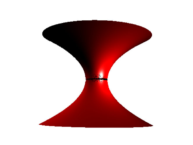
Figure 1: The Riemannian surface ${\cal S}$: the Flamm’s paraboloid.

II.0.1 The Flamm’s paraboloid $\cal S$

The surface ${\cal S}$ whose local geometry is fixed by the metric (1) is known as the Flamm’s paraboloid. It is composed by two identical “universes”: ${\cal S}_{+}$ the one at $Z>0$, and ${\cal S}_{-}$ the one at $Z<0$. These are both multiply connected surfaces with the “Schwarzschild wormhole” providing the path from one to the other.

The system of coordinates $(r,\varphi)$ with the metric (1) has the disadvantage that it requires two charts to cover the whole surface ${\cal S}$. It can be more convenient to use the variable

$$u=\frac{Z}{4M}=\pm\sqrt{\frac{r}{2M}-1}$$ (4)

instead of $r$. Replacing $r$ as a function of $Z$ using equation (3) gives the following metric when using the system of coordinates $(u,\varphi)$,

$$d\mathbf{s}^{2}=4M^{2}(1+u^{2})\left[4\,du^{2}+(1+u^{2})\,d\varphi^{2}\right]~{}.$$ (5)

The region $u>0$ corresponds to ${\cal S}_{+}$ and the region $u<0$ to ${\cal S}_{-}$.

Let us consider that the OCP is confined in a “disk” defined as

$$\Omega_{R}^{+}=\{{\bf q}=(r,\varphi)\in{\cal S}_{+}|0\leq\varphi\leq 2\pi,2M\leq r\leq R\}~{}.$$ (6)

The area of this disk is given by

$$\mathcal{A}_{R}=\int_{\Omega_{R}}dS=\pi\left[\sqrt{R(R-2M)}(3M+R)+6M^{2}\ln\left(\frac{\sqrt{R}+\sqrt{R-2M}}{\sqrt{2M}}\right)\right]~{},$$ (7)

where $dS=\sqrt{g}\,dr\,d\varphi$ and $g=\det(g_{\mu\nu})$. The perimeter is $\mathcal{C}_{R}=2\pi R$.

The Riemann tensor in a two dimensional space has only $2^{2}(2^{2}-1)/12=1$ independent component. In our case the characteristic component is

$${R^{r}}_{\varphi r\varphi}=-\frac{M}{r}~{}.$$ (8)

The scalar curvature is then given by the following indexes contractions

$$\mathcal{R}={R^{\mu}}_{\mu}={R^{\mu\nu}}_{\mu\nu}=2{R^{r\varphi}}_{r\varphi}=2g^{\varphi\varphi}{R^{r}}_{\varphi r\varphi}=-\frac{2M}{r^{3}}~{},$$ (9)

and the (intrinsic) Gaussian curvature is $K=\mathcal{R}/2=-M/r^{3}$. The (extrinsic) mean curvature of the manifold turns out to be $H=-\sqrt{M/8r^{3}}$.

The Euler characteristic of the disk $\Omega_{R}^{+}$ is given by

$$\chi=\frac{1}{2\pi}\left(\int_{\Omega_{R}^{+}}K\,dS+\int_{\partial\Omega_{R}^{+}}k\,dl\right)~{},$$ (10)

where $k$ is the geodesic curvature of the boundary $\partial\Omega_{R}^{+}$. The Euler characteristic turns out to be zero, in agreement with the Gauss-Bonnet theorem $\chi=2-2h-b$ where $h=0$ is the number of handles and $b=2$ the number of boundaries.

We can also consider the case where the system is confined in a “double” disk

$$\Omega_{R}=\Omega_{R}^{+}\cup\Omega_{R}^{-}\,,$$ (11)

with $\Omega_{R}^{-}=\{{\bf q}=(r,\varphi)\in{\cal S}_{-}|0\leq\varphi\leq 2\pi,2M\leq r\leq R\}$, the disk image of $\Omega_{R}^{+}$ on the lower universe ${\cal S}_{-}$ portion of ${\cal S}$. The Euler characteristic of $\Omega_{R}$ is also $\chi=0$.

II.0.2 A useful system of coordinates

The Laplacian for a function $f$ is

$$\Delta f = \frac{1}{\sqrt{g}}\frac{\partial}{\partial q^{\mu}}\left(\sqrt{g}\,g^{\mu\nu}\frac{\partial}{\partial q^{\nu}}\right)f$$ (12)

$$= \left[\left(1-\frac{2M}{r}\right)\frac{\partial^{2}}{\partial r^{2}}+\frac{1}{r^{2}}\frac{\partial^{2}}{\partial\varphi^{2}}+\left(\frac{1}{r}-\frac{M}{r^{2}}\right)\frac{\partial}{\partial r}\right]f~{},$$

where ${\bf q}\equiv(r,\varphi)$. In appendix A, we show how, finding the Green function of the Laplacian, naturally leads to consider the system of coordinates $(x,\varphi)$, with

$$x=(\sqrt{u^{2}+1}+u)^{2}\,.$$ (13)

The range for the variable $x$ is $\left]0,+\infty\right[$. The lower paraboloid ${\cal S}_{-}$ corresponds to the region $0<x<1$ and the upper one ${\cal S}_{+}$ to the region $x>1$. A point in the upper paraboloid with coordinate $(x,\varphi)$ has a mirror image by reflection ($u\to-u$) in the lower paraboloid, with coordinates $(1/x,\varphi)$, since if

$$x=(\sqrt{u^{2}+1}+u)^{2}$$ (14)

then

$$\frac{1}{x}=(\sqrt{u^{2}+1}-u)^{2}\,.$$ (15)

In the upper paraboloid ${\cal S}_{+}$, the new coordinate $x$ can be expressed in terms of the original one, $r$, as

$$x=\frac{(\sqrt{r}+\sqrt{r-2M})^{2}}{2M}\,.$$ (16)

Using this system of coordinates, the metric takes the form of a flat metric multiplied by a conformal factor

$$d\mathbf{s}^{2}=\frac{M^{2}}{4}\left(1+\frac{1}{x}\right)^{4}\left(dx^{2}+x^{2}\,d\varphi^{2}\right)\,.$$ (17)

The Laplacian also takes a simple form

$$\Delta f=\frac{4}{M^{2}\left(1+\frac{1}{x}\right)^{4}}\,\Delta_{\mathrm{flat}}f$$ (18)

where

$$\Delta_{\mathrm{flat}}f=\frac{\partial^{2}f}{\partial x^{2}}+\frac{1}{x}\frac{\partial f}{\partial x}+\frac{1}{x^{2}}\frac{\partial^{2}f}{\partial\varphi^{2}}$$ (19)

is the Laplacian of the flat Euclidean space $\mathbb{R}^{2}$. The determinant of the metric is now given by $g=[M^{2}x(1+x^{-1})^{4}/4]^{2}$.

With this system of coordinates $(x,\varphi)$, the area of a “disk” $\Omega_{R}^{+}$ of radius $R$ [in the original system $(r,\varphi)$] is given by

$$\mathcal{A}_{R}=\frac{\pi M^{2}}{4}\,p(x_{m})$$ (20)

with

$$p(x)=x^{2}+8x-\frac{8}{x}-\frac{1}{x^{2}}+12\ln x$$ (21)

and $x_{m}=(\sqrt{R}+\sqrt{R-2M})^{2}/(2M)$.

III Coulomb potential

III.1 Coulomb potential created by a point charge

The Coulomb potential $G(x,\varphi;x_{0},\varphi_{0})$ created at $(x,\varphi)$ by a unit charge at $(x_{0},\varphi_{0})$ is given by the Green function of the Laplacian

$$\Delta G(x,\varphi;x_{0},\varphi_{0})=-2\pi\delta^{(2)}(x,\varphi;x_{0},\varphi_{0})$$ (22)

with appropriate boundary conditions. The Dirac distribution is given by

$$\delta^{(2)}(x,\varphi;x_{0},\varphi_{0})=\frac{4}{M^{2}x(1+x^{-1})^{4}}\,\delta(x-x_{0})\delta(\varphi-\varphi_{0})$$ (23)

Notice that using the system of coordinates $(x,\varphi)$ the Laplacian Green function equation takes the simple form

$$\Delta_{\mathrm{flat}}G(x,\varphi;x_{0},\varphi_{0})=-2\pi\frac{1}{x}\,\delta(x-x_{0})\delta(\varphi-\varphi_{0})$$ (24)

which is formally the same Laplacian Green function equation for flat space.

We shall consider three different situations: when the particles can be in the whole surface ${\cal S}$, or when the particles are confined to the upper paraboloid universe ${\cal S}_{+}$, confined by a hard wall or by a grounded perfect conductor.

III.1.1 Coulomb potential $G^{\mathrm{ws}}$ when the particles live in the whole surface ${\cal S}$

To complement the Laplacian Green function equation (22), we impose the usual boundary condition that the electric field $-\nabla G$ vanishes at infinity ($x\to\infty$ or $x\to 0$). Also, we require the usual interchange symmetry $G(x,\varphi;x_{0},\varphi_{0})=G(x_{0},\varphi_{0};x,\varphi)$ to be satisfied. Additionally, due to the symmetry between each universe ${\cal S}_{+}$ and ${\cal S}_{-}$, we require that the Green function satisfies the symmetry relation

$$G^{\mathrm{ws}}(x,\varphi;x_{0},\varphi_{0})=G^{\mathrm{ws}}(1/x,\varphi;1/x_{0},\varphi_{0})$$ (25)

The Laplacian Green function equation (22) can be solved, as usual, by using the decomposition as a Fourier series. Since equation (22) reduces to the flat Laplacian Green function equation (24), the solution is the standard one

$$G(x,\varphi;x_{0},\varphi_{0})=\sum_{n=1}^{\infty}\frac{1}{n}\left(\frac{x_{<}}{x_{>}}\right)^{2n}\cos\left[n(\varphi-\varphi_{0})\right]+g_{0}(x,x_{0})$$ (26)

where $x_{>}=\max(x,x_{0})$ and $x_{<}=\min(x,x_{0})$. The Fourier coefficient for $n=0$, has the form

$$g_{0}(x,x_{0})=\begin{cases}a_{0}^{+}\ln x+b_{0}^{+}\,,&x>x_{0}\\ a_{0}^{-}\ln x+b_{0}^{-}\,,&x<x_{0}\,.\end{cases}$$ (27)

The coefficients $a_{0}^{\pm},b_{0}^{\pm}$ are determined by the boundary conditions that $g_{0}$ should be continuous at $x=x_{0}$, its derivative discontinuous $\partial_{x}g_{0}|_{x=x_{0}^{+}}-\partial_{x}g_{0}|_{x=x_{0}^{-}}=-1/x_{0}$, and the boundary condition at infinity $\nabla g_{0}|_{x\to\infty}=0$ and $\nabla g_{0}|_{x\to 0}=0$. Unfortunately, the boundary condition at infinity is trivially satisfied for $g_{0}$, therefore $g_{0}$ cannot be determined only with this condition. In flat space, this is the reason why the Coulomb potential can have an arbitrary additive constant added to it. However, in our present case, we have the additional symmetry relation (25) which should be satisfied. This fixes the Coulomb potential up to an additive constant $b_{0}$. We find

$$g_{0}(x,x_{0})=-\frac{1}{2}\ln\frac{x_{>}}{x_{<}}+b_{0}\,,$$ (28)

and summing explicitly the Fourier series (26), we obtain

$$G^{\mathrm{ws}}(x,\varphi;x_{0},\varphi_{0})=-\ln\frac{\left|z-z_{0}\right|}{\sqrt{\left|zz_{0}\right|}}+b_{0}~{},$$ (29)

where we defined $z=xe^{i\varphi}$ and $z_{0}=x_{0}e^{i\varphi_{0}}$. Notice that this potential does not reduce exactly to the flat one when $M=0$. This is due to the fact that the whole surface $\mathcal{S}$ in the limit $M\to 0$ is not exactly a flat plane $\mathbb{R}^{2}$, but rather it is two flat planes connected by a hole at the origin, this hole modifies the Coulomb potential.

III.1.2 Coulomb potential $G^{\mathrm{hs}}$ when the particles live in the half surface ${\cal S}_{+}$ confined by hard walls

We consider now the case when the particles are restricted to live in the half surface ${\cal S}_{+}$, $x>1$, and they are confined by a hard wall located at the “horizon” $x=1$. The region $x<1$ (${\cal S}_{-}$) is empty and has the same dielectric constant as the upper region occupied by the particles. Since there are no image charges, the Coulomb potential is the same $G^{\mathrm{ws}}$ as above. However, we would like to consider here a new model with a slightly different interaction potential between the particles. Since we are dealing only with half surface, we can relax the symmetry condition (25). Instead, we would like to consider a model where the interaction potential reduces to the flat Coulomb potential in the limit $M\to 0$. The solution of the Laplacian Green function equation is given in Fourier series by equation (26). The zeroth order Fourier component $g_{0}$ can be determined by the requirement that, in the limit $M\to 0$, the solution reduces to the flat Coulomb potential

$$G^{\mathrm{flat}}({\bf r},{\bf r}^{\prime})=-\ln\frac{|{\bf r}-{\bf r}^{\prime}|}{L}$$ (30)

where $L$ is an arbitrary constant length. Recalling that $x\sim 2r/M$, when $M\to 0$, we find

$$g_{0}(x,x_{0})=-\ln x_{>}-\ln\frac{M}{2L}$$ (31)

and

$$G^{\mathrm{hs}}(x,\varphi;x_{0},\varphi_{0})=-\ln|z-z_{0}|-\ln\frac{M}{2L}\,.$$ (32)

III.1.3 Coulomb potential $G^{\mathrm{gh}}$ when the particles live in the half surface ${\cal S}_{+}$ confined by a grounded perfect conductor

Let us consider now that the particles are confined to ${\cal S}_{+}$ by a grounded perfect conductor at $x=1$ which imposes Dirichlet boundary condition to the electric potential. The Coulomb potential can easily be found from the Coulomb potential $G^{\mathrm{ws}}$ (29) using the method of images

$$G^{\mathrm{gh}}(x,\varphi;x_{0},\varphi_{0})=-\ln\frac{|z-z_{0}|}{\sqrt{|zz_{0}|}}+\ln\frac{|z-\bar{z}_{0}^{-1}|}{\sqrt{|z\bar{z}_{0}^{-1}|}}=-\ln\left|\frac{z-z_{0}}{1-z\bar{z}_{0}}\right|$$ (33)

where the bar over a complex number indicates its complex conjugate. We will call this the grounded horizon Green function. Notice how its shape is the same of the Coulomb potential on the pseudosphere R. Fantoni, B. Jancovici, and G. Téllez (2003) or in a flat disk confined by perfect conductor boundaries B. Jancovici and G. Téllez (1996).

This potential can also be found using the Fourier decomposition. Since it will be useful in the following, we note that the zeroth order Fourier component of $G^{\mathrm{gh}}$ is

$$g_{0}(x,x_{0})=\ln x_{<}\,.$$ (34)

III.2 The background

The Coulomb potential generated by the background, with a constant surface charge density $\rho_{b}$ satisfies the Poisson equation

$$\Delta v_{b}=-2\pi\rho_{b}\,.$$ (35)

Assuming that the system occupies an area $\mathcal{A}_{R}$, the background density can be written as $\rho_{b}=-qN_{b}/\mathcal{A}_{R}=-qn_{b}$, where we have defined here $n_{b}=N_{b}/\mathcal{A}_{R}$ the number density associated to the background. For a neutral system $N_{b}=N$. The Coulomb potential of the background can be obtained by solving Poisson equation with the appropriate boundary conditions for each case. Also, it can be obtained from the Green function computed in the previous section

$$v_{b}(x,\varphi)=\int G(x,\varphi;x^{\prime},\varphi^{\prime})\rho_{b}\,dS^{\prime}\,.$$ (36)

This integral can be performed easily by using the Fourier series decomposition (26) of the Green function $G$. Recalling that $dS=\frac{1}{4}M^{2}x(1+x^{-1})^{4}\,dx\,d\varphi$, after the angular integration is done, only the zeroth order term in the Fourier series survives

$$v_{b}(x,\varphi)=\frac{\pi\rho_{b}M^{2}}{2}\int_{1}^{x_{m}}g_{0}(x,x^{\prime})\,x\left(1+\frac{1}{x}\right)^{4}\,dx\,.$$ (37)

The previous expression is for the half surface case and the grounded horizon case. For the whole surface case, the lower limit of integration should be replaced by $1/x_{m}$, or, equivalently, the integral multiplied by a factor 2.

Using the explicit expressions for $g_{0}$, (28), (31), and (34) for each case, we find, for the whole surface,

$$v_{b}^{\mathrm{ws}}(x,\varphi)=-\frac{\pi\rho_{b}M^{2}}{8}\left[h(x)-h(x_{m})+2p(x_{m})\ln x_{m}-4b_{0}p(x_{m})\right]$$ (38)

where $p(x)$ was defined in equation (21), and

$$h(x)=x^{2}+16x+\frac{16}{x}+\frac{1}{x^{2}}+12(\ln x)^{2}-34\,.$$ (39)

Notice the following properties satisfied by the functions $p$ and $h$

$$p(x)=-p(1/x)\,,\qquad h(x)=h(1/x)$$ (40)

and

$$p(x)=xh^{\prime}(x)/2\,,\qquad p^{\prime}(x)=2x\left(1+\frac{1}{x}\right)^{4}$$ (41)

where the prime stands for the derivative.

The background potential for the half surface case, with the pair potential $-\ln(|z-z^{\prime}|M/2L)$ is

$$v_{b}^{\mathrm{hs}}(x,\varphi)=-\frac{\pi\rho_{b}M^{2}}{8}\left[h(x)-h(x_{m})+2p(x_{m})\ln\frac{x_{m}M}{2L}\right]\,.$$ (42)

Also, the background potential in the half surface case, but with the pair potential $-\ln(|z-z^{\prime}|/\sqrt{|zz^{\prime}|})+b_{0}$ is

$$v_{b}^{\overline{\mathrm{hs}}}(x,\varphi)=-\frac{\pi\rho_{b}M^{2}}{8}\left[h(x)-\frac{h(x_{m})}{2}+p(x_{m})\left(\ln\frac{x_{m}}{x}-2b_{0}\right)\right]\,.$$ (43)

Finally, for the grounded horizon case,

$$v_{b}^{\mathrm{gh}}(x,\varphi)=-\frac{\pi\rho_{b}M^{2}}{8}\left[h(x)-2p(x_{m})\ln x\right]\,.$$ (44)

IV Partition function and density at $\Gamma=2$

We will now show how at the special value of the coupling constant $\Gamma=\beta q^{2}=2$ the partition function and $n$-body correlation functions can be calculated exactly.

In the following we will distinguish four cases labeled by $A$: $A=\rm{hs}$, the plasma on the half surface (choosing $G^{\rm{hs}}$ as the pair Coulomb potential); $A=\rm{ws}$, the plasma on the whole surface (choosing $G^{\rm{ws}}$ as the pair Coulomb potential); $A=\overline{\rm{hs}}$, the plasma on the half surface but with the Coulomb potential $G^{\rm{ws}}$ of the whole surface case; and $A=\rm{gh}$, the plasma on the half surface with the grounded horizon (choosing $G^{\rm{gh}}$ as the pair Coulomb potential).

The total potential energy of the plasma is, in each case

$$V^{A}=v_{0}^{A}+q\sum_{i}v_{b}^{A}(x_{i})+q^{2}\sum_{i<j}G^{A}(x_{i},\varphi_{i};x_{j},\varphi_{j})~{},$$ (45)

where $(x_{i},\varphi_{i})$ is the position of charge $i$ on the surface, and

$$v_{0}^{A}=\frac{1}{2}\int\rho_{b}v_{b}^{A}(x,\varphi)\,dS$$ (46)

is the self energy of the background in each of the four mentioned cases. In the grounded case $A=\text{gh}$, one should add to $V^{\text{gh}}$ in (45) the self energy that each particle has due to the polarization it creates on the grounded conductor.

IV.1 The 2dOCP on half surface with potential $-\ln|z-z^{\prime}|-\ln M/(2L)$

IV.1.1 Partition function

For this case, we work in the canonical ensemble with $N$ particles and the background neutralizes the charges: $N_{b}=N$, and $n=N/\mathcal{A}_{R}=n_{b}$. The potential energy of the system takes the explicit form

$$V^{\mathrm{hs}} = -q^{2}\sum_{1\leq i<j\leq N}\ln|z_{i}-z_{j}|+\frac{q^{2}}{2}\alpha\sum_{i=1}^{N}h(x_{i})+\frac{q^{2}}{2}N\ln\frac{M}{2L}-\frac{q^{2}}{4}N\alpha h(x_{m})$$ (47)

$$+\frac{q^{2}}{2}N^{2}\ln x_{m}-\frac{q^{2}}{4}\alpha^{2}\int_{1}^{x_{m}}h(x)p^{\prime}(x)\,dx$$

where we have used the fact that $dS=\pi M^{2}x(1+x^{-1})^{4}\,dx/2=\pi M^{2}p^{\prime}(x)\,dx/4$, and we have defined

$$\alpha=\frac{\pi n_{b}M^{2}}{4}\,.$$ (48)

Integrating by parts the last term of (47) and using (41), we find

$$V^{\mathrm{hs}} = -q^{2}\sum_{1\leq i<j\leq N}\ln|z_{i}-z_{j}|+\frac{q^{2}}{2}\alpha\sum_{i=1}^{N}h(x_{i})+\frac{q^{2}}{2}N\ln\frac{M}{2L}+\frac{q^{2}}{2}N^{2}\ln x_{m}$$ (49)

$$+\frac{q^{2}}{2}\alpha^{2}\int_{1}^{x_{m}}\frac{[p(x)]^{2}}{x}\,dx-\frac{q^{2}}{2}N\alpha h(x_{m})\,.$$

When $\beta q^{2}=2$, the canonical partition function can be written as

$$Z^{\mathrm{hs}}=\frac{1}{\lambda^{2N}}\,Z_{0}^{\mathrm{hs}}\exp(-\beta F_{0}^{\mathrm{hs}})$$ (50)

with

$$-\beta F_{0}^{\mathrm{hs}}=-N\ln\frac{M}{2L}-N^{2}\ln x_{m}-\alpha^{2}\int_{1}^{x_{m}}\frac{[p(x)]^{2}}{x}\,dx+N\alpha h(x_{m})$$ (51)

and

$$Z_{0}^{\mathrm{hs}}=\frac{1}{N!}\int\prod_{i=1}^{N}dS_{i}\,e^{-\alpha h(x_{i})}\prod_{1\leq i<j\leq N}|z_{i}-z_{j}|^{2}\,.$$ (52)

where $\lambda=\sqrt{2\pi\beta\hbar^{2}/m}$ is the de Broglie thermal wavelength. $Z_{0}$ can be computed using the original method for the OCP in flat space Jancovici (1981); A. Alastuey and B. Jancovici (1981), which was originally introduced in the context of random matrices M. L. Mehta (1991); Ginibre (1965). By expanding the Vandermonde determinant $\prod_{i<j}(z_{i}-z_{j})$ and performing the integration over the angles, the partition function can be written as

$$Z_{0}^{\mathrm{hs}} = \prod_{k=0}^{N-1}{\cal B}_{N}(k)~{},$$ (53)

where

$${\cal B}_{N}(k) = \int x^{2k}e^{-\alpha h(x)}\,dS$$ (54)

$$= \frac{\alpha}{n_{b}}\int_{1}^{x_{m}}x^{2k}e^{-\alpha h(x)}p^{\prime}(x)\,dx\,.$$ (55)

In the flat limit $M\to 0$, we have $x\sim 2r/M$, with $r$ the radial coordinate of the flat space $\mathbb{R}^{2}$, and $h(x)\sim p(x)\sim x^{2}$. Then, $\mathcal{B}_{N}$ reduces to

$$\mathcal{B}_{N}(k)\sim\frac{1}{n_{b}\alpha^{k}}\,\gamma(k+1,N)$$ (56)

where $\gamma(k+1,N)=\int_{0}^{N}t^{k}e^{-t}\,dt$ is the incomplete Gamma function. Replacing into (53), we recover the partition function for the OCP in a flat disk of radius $R$ A. Alastuey and B. Jancovici (1981)

$$\ln Z^{\mathrm{hs}}=\frac{N}{2}\ln\frac{\pi L^{2}}{n_{b}\lambda^{4}}+\frac{3N^{2}}{4}-\frac{N^{2}}{2}\ln N+\sum_{k=1}^{N}\ln\gamma(k,N)\,.$$ (57)

IV.1.2 Thermodynamic limit $R\to\infty$, $x_{m}\to\infty$, and fixed $M$

Let us consider the limit of a large system when $x_{m}=(\sqrt{R}+\sqrt{R-2M})^{2}/(2M)\to\infty$, $N\to\infty$, constant density $n$, and constant $M$. Therefore $\alpha$ is also kept constant. In appendix B, we develop a uniform asymptotic expansion of $\mathcal{B}_{N}(k)$ when $N\to\infty$ and $k\to\infty$ with $(N-k)/\sqrt{N}=O(1)$. Let us define $\hat{x}_{k}$ by

$$k=\alpha p(\hat{x}_{k})\,.$$ (58)

The asymptotic expansion (225) of $\mathcal{B}_{N}(k)$ can be rewritten as

$$\mathcal{B}_{N}(k) = \frac{1}{2n_{b}}\sqrt{\pi\alpha\hat{x}_{k}p^{\prime}(\hat{x}_{k})}\,e^{2k\ln\hat{x}_{k}-\alpha h(\hat{x}_{k})}\left[1+\mathop{\text{missing}}{erf}\left(\epsilon_{k}\right)\right]$$ (59)

$$\times\left[1+\frac{1}{12k}+\frac{1}{\sqrt{k}}\,\xi_{1}(\epsilon_{k})+\frac{1}{k}\,\xi_{2}(\epsilon_{k})\right]$$

where

$$\epsilon_{k}=\frac{2p(x_{k})}{x_{k}p^{\prime}(x_{k})}\frac{N-k}{\sqrt{2k}}$$ (60)

is a order one parameter, and the functions $\xi_{1}(\epsilon_{k})$ and $\xi_{2}(\epsilon_{k})$ can be obtained from the calculation presented in appendix B. They are integrable functions for $\epsilon_{k}\in[0,\infty[$. We will obtain an expansion of the free energy up to the order $\ln N$. At this order the functions $\xi_{1,2}$ do not contribute to the result.

Writing down

$$\ln Z_{0}^{\mathrm{hs}}=\sum_{k=0}^{N}\ln\mathcal{B}_{N}(k)-\ln\mathcal{B}_{N}(N)$$ (61)

and using the asymptotic expansion (59), we have

$$\ln Z_{0}^{\mathrm{hs}} = -N\ln\frac{n_{b}}{\sqrt{2\pi}}+S_{1}^{\mathrm{hs}}+S_{2}^{\mathrm{hs}}+S_{3}^{\mathrm{hs}}+\frac{1}{12}\ln N$$ (62)

$$-\ln\left[\sqrt{\alpha}x_{m}\left(1+\frac{1}{x_{m}}\right)^{2}\right]-2N\ln x_{m}+\alpha h(x_{m})+O(1)$$

with

$$S_{1}^{\mathrm{hs}} = \sum_{k=0}^{N}\ln\left(\sqrt{\alpha}\hat{x}_{k}\left(1+\frac{1}{\hat{x}_{k}}\right)^{2}\right]$$ (63)

$$S_{2}^{\mathrm{hs}} = \sum_{k=0}^{N}\left[2k\ln\hat{x}_{k}-\alpha h(\hat{x}_{k})\right]$$ (64)

$$S_{3}^{\mathrm{hs}} = \sum_{k=0}^{N}\ln\frac{1+\mathop{\text{missing}}{erf}\left(\epsilon_{k}\right)}{2}\,.$$ (65)

Notice that the contribution of $\xi_{1}(\epsilon_{k})$ is of order one, since $\sum_{k}\xi_{1}(\epsilon_{k})/\sqrt{k}\sim\int_{0}^{\infty}\xi_{1}(\epsilon)\,d\epsilon=O(1)$. Also, $\sum_{k}\xi_{2}(\epsilon_{k})/k\sim(1/\sqrt{N})\int_{0}^{\infty}\xi_{2}(\epsilon)\,d\epsilon=O(1/\sqrt{N})$.

$S_{3}^{\mathrm{hs}}$ gives a contribution of order $\sqrt{N}$, transforming the sum over $k$ into an integral over the variable $t=\epsilon_{k}$, we have

$$S_{3}=\sqrt{2N}\int_{0}^{\infty}\ln\frac{1+\mathop{\text{missing}}{erf}(t)}{2}\,dt+O(1)\,.$$ (66)

This contribution is the same as the perimeter contribution in the flat case.

To expand $S_{1}^{\mathrm{hs}}$ and $S_{2}^{\mathrm{hs}}$ up to order $O(1)$, we need to use the Euler-McLaurin summation formula M. Abramowitz and A. Stegun (1965); R. Wong (1989)

$$\sum_{k=0}^{N}f(k)=\int_{0}^{N}f(y)\,dy+\frac{1}{2}\left[f(0)+f(N)\right]+\frac{1}{12}\left[f^{\prime}(N)-f^{\prime}(0)\right]+\cdots\,.$$ (67)

We find

$$S_{1}^{\mathrm{hs}} = \frac{N}{2}\ln\alpha+\alpha x_{m}^{2}\left(\ln x_{m}-\frac{1}{2}\right)+\alpha x_{m}\left(8\ln x_{m}-4\right)$$ (68)

$$+\left(14\alpha+\frac{1}{2}\right)\ln x_{m}+6\left(\ln x_{m}\right)^{2}$$

and

$$S_{2}^{\mathrm{hs}} = N^{2}\ln x_{m}+N\ln x_{m}-\alpha Nh(x_{m})+\alpha^{2}\int_{1}^{x_{m}}\frac{\left[p(x)\right]^{2}}{x}\,dx-\frac{\alpha}{2}\,h(x_{m})+\frac{1}{6}\ln x_{m}\,.$$ (69)

Summing all terms in $\ln Z_{0}^{\mathrm{hs}}$ and those from $\beta F_{0}^{\mathrm{hs}}$, we notice that all nonextensive terms cancel, as it should be, and we obtain

$$\ln Z^{\mathrm{hs}}=-N\beta f_{B}+4x_{m}\alpha-\mathcal{C}_{R}\,\beta\gamma_{\text{hard}}+\left(14\alpha-\frac{1}{6}\right)\ln x_{m}+O(1)$$ (70)

where

$$\beta f_{B}=-\frac{1}{2}\ln\frac{2\pi^{2}L^{2}}{n\lambda^{4}}$$ (71)

is the bulk free energy of the OCP in the flat geometry A. Alastuey and B. Jancovici (1981),

$$\beta\gamma_{\text{hard}}=-\sqrt{\frac{n_{b}}{2\pi}}\int_{0}^{\infty}\ln\frac{1+\mathop{\text{missing}}{erf}(y)}{2}\,dy$$ (72)

is the perimeter contribution to the free energy (“surface” tension) in the flat geometry near a plane hard wall B. Jancovici, G. Manificat, and C. Pisani (1994), and

$$\mathcal{C}_{R}=2\pi R=\pi M\sqrt{x_{m}p^{\prime}(x_{m})/2}=\pi Mx_{m}+O(1)$$ (73)

is the perimeter of the boundary at $x=x_{m}$.

The region $x\to\infty$ has zero curvature, therefore in the limit $x_{m}\to\infty$, most of the system occupies an almost flat region. For this reason, the extensive term (proportional to $N$) is expected to be the same as the one in flat space $f_{B}$. The largest boundary of the system $x=x_{m}$ is also in an almost flat region, therefore it is not surprising to see the factor $\gamma_{\text{hard}}$ from the flat geometry appear there as well. Nevertheless, we notice an additional contribution $4\alpha x_{m}$ to the perimeter contribution, which comes from the curvature of the system. In the logarithmic correction $\ln x_{m}$, we notice a $-(1/6)\ln x_{m}$ term, the same as in a flat disk geometry B. Jancovici, G. Manificat, and C. Pisani (1994), but also a nonuniversal contribution due to the curvature $14\alpha\ln x_{m}$.

IV.1.3 Thermodynamic limit at fixed shape: $\alpha\to\infty$ and $x_{m}$ fixed

In the previous section we studied a thermodynamic limit case where a large part of the space occupied by the particles becomes flat as $x\to\infty$ keeping $M$ fixed. Another interesting thermodynamic limit that can be studied is the one where we keep the shape of the space occupied by the particles fixed. This limit corresponds to the situation $M\to\infty$ and $R\to\infty$ while keeping the ratio $R/M$ fixed, and of course the number of particles $N\to\infty$ with the density $n$ fixed. Equivalently, recalling that $N=\alpha p(x_{m})$, in this limit $x_{m}$ is fixed and finite, and $\alpha=\pi M^{2}n_{b}/4\to\infty$. We shall use $\alpha$ as the large parameter for the expansion of the free energy. In this limit, we expect the curvature effects to remain important, in particular the bulk free energy (proportional to $\alpha$) will not be the same as in flat space.

Using the expansion (228) of $\mathcal{B}_{N}(k)$ for the fixed shape situation, we have

$$\ln Z_{0}^{\mathrm{hs}}=N\ln\frac{\sqrt{\pi}}{n_{b}}+N\ln\sqrt{\alpha}+S_{1}^{\mathrm{hs,fixed}}+S_{2}^{\mathrm{hs,fixed}}+S_{3}^{\mathrm{hs,fixed}}+O(1)$$ (74)

where now

$$S_{1}^{\mathrm{hs,fixed}} = \frac{1}{2}\sum_{k=0}^{N-1}\ln[\hat{x}_{k}p^{\prime}(\hat{x}_{k})]$$ (75)

$$S_{2}^{\mathrm{hs,fixed}} = -\alpha\sum_{k=0}^{N-1}[h(\hat{x}_{k})-2p(\hat{x}_{k})\ln\hat{x}_{k}]$$ (76)

$$S_{3}^{\mathrm{hs,fixed}} = \sum_{k=0}^{N-1}\ln\frac{\mathop{\text{missing}}{erf}(\epsilon_{k,1})+\mathop{\text{missing}}{erf}(\epsilon_{k,m})}{2}$$ (77)

with $\epsilon_{k,m}$ and $\epsilon_{k,1}$ given in equations (229) and (230), and $\hat{x}_{k}$ is given by $k=\alpha p(\hat{x}_{k})$. Using the Euler-McLaurin expansion, we obtain

$$S_{1}^{\mathrm{hs,fixed}} = \alpha\int_{1}^{x_{m}}\frac{(1+x)^{4}}{x^{3}}\,\ln\frac{2(x+1)^{4}}{x^{2}}\,dx+O(1)$$ (78)

$$S_{2}^{\mathrm{hs,fixed}} = N^{2}\ln x_{m}-\alpha Nh(x_{m})+\alpha^{2}\int_{1}^{x_{m}}\frac{[p(x)]^{2}}{x}\,dx+\frac{\alpha}{2}h(x_{m})-N\ln x_{m}+O(1)\,.$$ (79)

For $S_{3}^{\mathrm{hs,fixed}}$, the relevant contributions are obtained when $k$ is of order $\sqrt{N}$, where $\epsilon_{k,1}$ is of order one, and when $N-k$ is of order $\sqrt{N}$, where $\epsilon_{k,m}$ is of order one. In those regions, the sum can be changed into an integral over the variable $t=\epsilon_{k,1}$ or $t=\epsilon_{k,m}$. This gives

$$S_{3}^{\mathrm{hs,fixed}} = -\sqrt{\frac{4\pi\alpha}{n_{b}}}\,\left[x_{m}\left(1+\frac{1}{x_{m}}\right)^{2}+4\right]\beta\gamma_{\text{hard}}+O(1)$$ (80)

with $\gamma_{\text{hard}}$ given in equation (72). Once again the nonextensive terms (proportional to $\alpha^{2}$) in $S_{2}^{\mathrm{hs,fixed}}$ cancel out with similar terms in $F_{0}^{\mathrm{hs,fixed}}$ from equation (51). The final result for the free energy $\beta F^{\mathrm{hs}}=-\ln Z^{\mathrm{hs}}$ is

$$\ln Z^{\mathrm{hs}} = \alpha\left[-p(x_{m})\beta f_{B}+\frac{1}{2}\left[h(x_{m})-2p(x_{m})\ln x_{m}\right]+\int_{1}^{x_{m}}\frac{(1+x)^{4}}{x^{3}}\,\ln\frac{(x+1)^{4}}{x^{2}}\,dx\right]$$ (81)

$$-\sqrt{\frac{4\pi\alpha}{n_{b}}}\,\left[x_{m}\left(1+\frac{1}{x_{m}}\right)^{2}+4\right]\beta\gamma_{\text{hard}}+O(1)$$

where $f_{B}$, given by (71), is the bulk free energy per particle in a flat space. We notice the additional contribution to the bulk free energy due to the important curvature effects [second and third term of the first line of equation (81)] that remain present in this thermodynamic limit.

The boundary terms, proportional to $\sqrt{\alpha}$, turn out to be very similar to those of a flat space near a hard wall B. Jancovici (1982), with a contribution $\beta\gamma_{\text{hard}}\mathcal{C}_{b}$ for each boundary at $x_{b}=x_{m}$ and at $x_{b}=1$ with perimeter

$$\mathcal{C}_{b}=\pi M\sqrt{\frac{x_{b}p^{\prime}(x_{b})}{2}}=\pi Mx_{b}\left(1+\frac{1}{x_{b}}\right)^{2}\,.$$ (82)

Also, we notice the absence of $\ln\alpha$ corrections in the free energy. This is in agreement with the general results from Refs. B. Jancovici, G. Manificat, and C. Pisani (1994); B. Jancovici and G. Téllez (1996), where, using arguments from conformal field theory, it is argued that for two-dimensional Coulomb systems living in a surface of Euler characteristic $\chi$, in the limit of a large surface keeping its shape fixed, the free energy should exhibit a logarithmic correction $(\chi/6)\ln R$ where $R$ is a characteristic length of the size of the surface. For our curved surface studied in this section, the Euler characteristic is $\chi=0$, therefore no logarithmic correction is expected.

IV.1.4 Distribution functions

Following Jancovici (1981), we can also find the $k$-body distribution functions

$$n^{(k){\mathrm{hs}}}({\bf q}_{1},\ldots,{\bf q}_{k})=\det[{\cal K}_{N}^{\mathrm{hs}}({\bf q}_{i},{\bf q}_{j})]_{(i,j)\in\{1,\ldots,k\}^{2}}~{},$$ (83)

where ${\bf q}_{i}=(x_{i},\varphi_{i})$ is the position of the particle $i$, and

$${\cal K}_{N}^{\mathrm{hs}}({\bf q}_{i},{\bf q}_{j})=\sum_{k=0}^{N-1}\frac{z_{i}^{k}\bar{z}_{j}^{k}e^{-\alpha[h(|z_{i}|)+h(|z_{j}|)]/2}}{{\cal B}_{N}(k)}~{}.$$ (84)

where $z_{k}=x_{k}e^{i\varphi_{k}}$. In particular, the one-body density is given by

$$n^{\mathrm{hs}}(x)=\mathcal{K}_{N}({\bf q},{\bf q})=\sum_{k=0}^{N-1}\frac{x^{2k}e^{-\alpha h(x)}}{\mathcal{B}_{N}(k)}\,.$$ (85)

IV.1.5 Internal screening

Internal screening means that at equilibrium, a particle of the system is surrounded by a polarization cloud of opposite charge. It is usually expressed in terms of the simplest of the multipolar sum rules Ph. A. Martin (1988): the charge or electroneutrality sum rule, which for the OCP reduces to the relation

$$\int n^{(2){\mathrm{hs}}}({\bf q}_{1},{\bf q}_{2})\,dS_{2}=(N-1)n^{(1){\mathrm{hs}}}({\bf q}_{1})~{},$$ (86)

This relation is trivially satisfied because of the particular structure (83) of the correlation function expressed as a determinant of the kernel $\mathcal{K}_{N}^{\mathrm{hs}}$, and the fact that $\mathcal{K}_{N}^{\mathrm{hs}}$ is a projector

$$\int dS_{3}\,\mathcal{K}_{N}^{\mathrm{hs}}({\bf q}_{1},{\bf q}_{3})\mathcal{K}_{N}^{\mathrm{hs}}({\bf q}_{3},{\bf q}_{2})=\mathcal{K}_{N}^{\mathrm{hs}}({\bf q}_{1},{\bf q}_{2})\,.$$ (87)

Indeed,

$$\int n^{(2){\mathrm{hs}}}({\bf q}_{1},{\bf q}_{2})\,dS_{2} = \int[{\cal K}_{N}^{\mathrm{hs}}({\bf q}_{1},{\bf q}_{1}){\cal K}_{N}^{\mathrm{hs}}({\bf q}_{2},{\bf q}_{2})-{\cal K}_{N}^{\mathrm{hs}}({\bf q}_{1},{\bf q}_{2}){\cal K}_{N}^{\mathrm{hs}}({\bf q}_{2},{\bf q}_{1})]\,dS_{2}$$ (88)

$$= \int n^{(1){\mathrm{hs}}}({\bf q}_{1})n^{(1){\mathrm{hs}}}({\bf q}_{2})\,dS_{2}-{\cal K}_{N}^{\mathrm{hs}}({\bf q}_{1},{\bf q}_{1})$$

$$= (N-1)n^{(1){\mathrm{hs}}}({\bf q}_{1})\,.$$

IV.1.6 External screening

External screening means that, at equilibrium, an external charge introduced into the system is surrounded by a polarization cloud of opposite charge. When an external infinitesimal point charge $Q$ is added to the system, it induces a charge density $\rho_{Q}({\bf q})$. External screening means that

$$\int\rho_{Q}({\bf q})\,dS=-Q~{}.$$ (89)

Using linear response theory we can calculate $\rho_{Q}$ to first order in $Q$ as follows. Imagine that the charge $Q$ is at ${\bf q}$. Its interaction energy with the system is $\hat{H}_{int}=Q\hat{\phi}({\bf q})$ where $\hat{\phi}({\bf q})$ is the microscopic electric potential created at ${\bf q}$ by the system. Then, the induced charge density at ${\bf q}^{\prime}$ is

$$\rho_{Q}({\bf q}^{\prime})=-\beta\langle\hat{\rho}({\bf q}^{\prime})\hat{H}_{int}\rangle_{T}=-\beta Q\langle\hat{\rho}({\bf q}^{\prime})\hat{\phi}({\bf q})\rangle_{T}~{},$$ (90)

where $\hat{\rho}({\bf q}^{\prime})$ is the microscopic charge density at ${\bf q}^{\prime}$, $\langle AB\rangle_{T}=\langle AB\rangle-\langle A\rangle\langle B\rangle$, and $\langle\ldots\rangle$ is the thermal average. Assuming external screening (89) is satisfied, one obtains the Carnie-Chan sum rule Ph. A. Martin (1988)

$$\beta\int\langle\hat{\rho}({\bf q}^{\prime})\hat{\phi}({\bf q})\rangle_{T}\,dS^{\prime}=1~{}.$$ (91)

Now in a uniform system starting from this sum rule one can derive the second moment Stillinger-Lovett sum rule Ph. A. Martin (1988). This is not possible here because our system is not homogeneous since the curvature is not constant throughout the surface but varies from point to point. If we apply the Laplacian respect to ${\bf q}$ to this expression and use Poisson equation

$$\Delta_{{\bf q}}\langle\hat{\rho}({\bf q}^{\prime})\hat{\phi}({\bf q})\rangle_{T}=-2\pi\langle\hat{\rho}({\bf q}^{\prime})\hat{\rho}({\bf q})\rangle_{T}~{},$$ (92)

we find

$$\int\rho_{e}^{(2)}({\bf q}^{\prime},{\bf q})\,dS^{\prime}=0~{},$$ (93)

where $\rho_{e}^{(2)}({\bf q}^{\prime},{\bf q})=\langle\hat{\rho}({\bf q}^{\prime})\hat{\rho}({\bf q})\rangle_{T}$ is the excess pair charge density function. Eq. (93) is another way of writing the charge sum rule Eq. (86) in the thermodynamic limit.

IV.1.7 Asymptotics of the density in the limit $x_{m}\to\infty$ and $\alpha$ fixed, for $1\ll x\ll x_{m}$

The formula (85) for the one-body density, although exact, does not allow a simple evaluation of the density at a given point in space, as one has first to calculate $\mathcal{B}_{N}(k)$ through an integral and then perform the sum over $k$. One can then try to determine the asymptotic behaviors of the density.

In this section, we consider the limit $x_{m}\to\infty$ and $\alpha$ fixed, and we study the density in the bulk of the system $1\ll x\ll x_{m}$.

In the sum (85), the dominant terms are the ones for which $k$ is such that $\hat{x}_{k}=x$, with $\hat{x}_{k}$ defined in (58). Since $1\ll x\ll x_{m}$, the dominant terms in the calculation of the density are obtained for values of $k$ such that $1\ll k\ll N$. Therefore in the limit $N\to\infty$, in the expansion (59) of $B_{N}(k)$, the argument of the error function is very large, then the error function can be replaced by 1. Keeping the correction $1/(12k)$ from (59) allow us to obtain an expansion of the density up to terms of order $O(1/x^{2})$. Replacing the sum over $k$ into an integral over $\hat{x}_{k}$, we have

$$n^{\text{hs}}(x)=\frac{n_{b}}{\sqrt{\pi}}\int_{-\infty}^{\infty}e^{\Psi(\hat{x}_{k})}f(\hat{x}_{k})\left(1-\frac{1}{12\alpha p(\hat{x}_{k})}\right)\,d\hat{x}_{k}$$ (94)

with

$$\Psi(\hat{x}_{k})=2\alpha p(\hat{x}_{k})\ln\frac{x}{\hat{x}_{k}}-\alpha[h(x)-h(\hat{x}_{k})]$$ (95)

and

$$f(\hat{x}_{k})=\sqrt{\frac{\alpha p^{\prime}(\hat{x}_{k})}{\hat{x}_{k}}}\,.$$ (96)

We proceed now to use the Laplace method to compute this integral. The function $\Psi(\hat{x}_{k})$ has a maximum for $x=\hat{x}_{k}$, with $\Psi(x)=0$ and

$$\Psi^{\prime\prime}(x) = -\frac{2\alpha p^{\prime}(x)}{x}$$ (97a)

$$\Psi^{(3)}(x) = -\frac{4\alpha}{x}+O(1/x^{2})$$ (97b)

$$\Psi^{(4)}(x) = \frac{4\alpha}{x^{2}}+O(1/x^{3})\,.$$ (97c)

Expanding for $\hat{x}_{k}$ close to $x$ and for $x\gg 1$ up to order $1/x^{2}$, we have

$$n^{\text{hs}}(x) = \frac{n_{b}}{\sqrt{\pi}}\int_{-\infty}^{+\infty}e^{-\alpha p^{\prime}(x)(\hat{x}_{k}-x)^{2}/x}\left(f(x)+f^{\prime}(x)(\hat{x}_{k}-x)+\frac{f^{\prime\prime}(x)(\hat{x}_{k}-x)^{2}}{2}\right)$$ (98)

$$\times\left(1+\frac{1}{3!}\Psi^{(3)}(x)(\hat{x}_{k}-x)^{3}+\frac{1}{4!}\Psi^{(4)}(x)(\hat{x}_{k}-x)^{4}+\frac{[\Psi^{(3)}(x)]^{2}}{3!^{2}\ 2}(\hat{x}_{k}-x)^{6}\right)$$

$$\times\left(1-\frac{1}{12\alpha p(x)}+O(1/x^{3})\right)\,d\hat{x}_{k}\,.$$

For the expansion of $f(\hat{x}_{k})$ around $\hat{x}_{k}=x$, it is interesting to notice that

$$f^{\prime}(x)=O(1/x^{2})\,,\qquad\text{and }f^{\prime\prime}(x)=O(1/x^{3})\,.$$ (99)

In the integral, the factor containing $f^{\prime}(x)$ is multiplied $(\hat{x}_{k}-x)$ which after integration vanishes. Therefore, the relevant contributions to order $O(1/x^{2})$ are

$$n^{\text{hs}}(x) = \frac{n_{b}}{\sqrt{\pi}}\int_{-\infty}^{+\infty}e^{-\alpha p^{\prime}(x)(\hat{x}_{k}-x)^{2}/x}\sqrt{\frac{\alpha p^{\prime}(x)}{x}}$$ (100)

$$\times\left(1+\frac{1}{3!}\Psi^{(3)}(x)(\hat{x}_{k}-x)^{3}+\frac{1}{4!}\Psi^{(4)}(x)(\hat{x}_{k}-x)^{4}+\frac{[\Psi^{(3)}(x)]^{2}}{3!^{2}\ 2}(\hat{x}_{k}-x)^{6}\right)$$

$$\times\left(1-\frac{1}{12\alpha p(x)}\right)\,d\hat{x}_{k}+O(1/x^{3})\,.$$

Then, performing the Gaussian integrals and replacing the dominant values of $\Psi(x)$ and its derivatives from Eqs. (97) for $x\gg 1$, we find

$$n(x)=n_{b}\left(1+\frac{1}{12\alpha x^{2}}\right)\left(1-\frac{1}{12\alpha x^{2}}\right)+O(1/x^{3})=n_{b}+O(1/x^{3})\,.$$ (101)

In the bulk of the plasma, the density of particles equal the bulk density, as expected. The above calculation, based the Laplace method, generates an expansion in powers of $1/x$ for the density. The first correction to the background density, in $1/x^{2}$, has been shown to be zero. We conjecture that this is probably true for any subsequent corrections in powers $1/x$ if the expansion is pushed further, because the corrections to the bulk density are probably exponentially small, rather than in powers of $1/x$, due to the screening effects. In the following subsections, we consider the expansion of the density in other types of limits, and in particular close to the boundaries, and the results suggest that our conjecture is true.

IV.1.8 Asymptotics of the density close to the boundary in the limit $x_{m}\to\infty$

We study here the density close to the boundary $x=x_{m}$ in the limit $x_{m}\to\infty$ and $M$ fixed. Since in this limit this region is almost flat, one would expect to recover the result for the OCP in a flat space near a wall B. Jancovici (1982). Let $x=x_{m}+y$ where $y\ll x_{m}$ is of order 1.

Using the dominant term of the asymptotics (59),

$$\mathcal{B}_{N}(k) = \frac{1}{2n_{b}}\sqrt{\pi\alpha\hat{x}_{k}p^{\prime}(\hat{x}_{k})}\,e^{2k\ln\hat{x}_{k}-\alpha h(\hat{x}_{k})}\left[1+\mathop{\text{missing}}{erf}\left({\epsilon_{k}}\right)\right]\,,$$ (102)

we have

$$n^{\mathrm{hs}}(x)=\frac{2n_{b}}{\sqrt{\pi}}\sum_{k=0}^{N-1}\frac{e^{2k(\ln x-\ln\hat{x}_{k})-\alpha[h(x)-h(\hat{x}_{k})]}}{\sqrt{\alpha\hat{x}_{k}p^{\prime}(\hat{x}_{k})}\left[1+\mathop{\text{missing}}{erf}\left({\epsilon_{k}}\right)\right]}$$ (103)

where we recall that $\hat{x}_{k}=p^{-1}(k/\alpha)$. The exponential term in the sum has a maximum when $\hat{x}_{k}=x$ i.e. $k=k_{\max}=\alpha p(x)$, and since $x$ is close to $x_{m}\to\infty$, the function is very peaked near this maximum. Thus, we can use Laplace method to compute the sum. Expanding the argument of the exponential up to order 2 in $k-k_{\max}$, we have

$$n^{\mathrm{hs}}(x)=\frac{2n_{b}}{\sqrt{\pi}}\sum_{k=0}^{N-1}\frac{\exp\left[-\frac{2}{\alpha xp^{\prime}(x)}(k-k_{\max})^{2}\right]}{\sqrt{\alpha xp^{\prime}(x)}\left[1+\mathop{\text{missing}}{erf}\left(\epsilon_{k}\right)\right]}$$ (104)

Now, replacing the sum by an integral over $t=\epsilon_{k}$ and replacing $x=x_{m}-y$, we find

$$n^{\mathrm{hs}}(x)=\frac{2n_{b}}{\sqrt{\pi}}\int_{0}^{\infty}\frac{\exp\left[-(t-\sqrt{2\alpha}y)^{2}\right]}{1+\mathop{\text{missing}}{erf}(t)}\,dt\,.$$ (105)

Since both $x_{m}\to\infty$, and $x\to\infty$, in that region, the space is almost flat. If $s$ is the geodesic distance from $x$ to the border, then we have $y\sim\sqrt{(\pi n_{b}/\alpha)}\,s$, and equation (105) reproduces the result for the flat space B. Jancovici (1982), as expected.

IV.1.9 Density in the thermodynamic limit at fixed shape: $\alpha\to\infty$ and $x_{m}$ fixed.

Using the expansion (228) of $\mathcal{B}_{N}(k)$ for the fixed shape situation, we have

$$n^{\mathrm{hs}}(x)=2n_{b}\sum_{k=0}^{N-1}\frac{e^{-\alpha[h(x)-2p(\hat{x}_{k})\ln x-h(\hat{x}_{k})+2p(\hat{x}_{k})\ln\hat{x}_{k}]}}{\sqrt{\alpha\pi\hat{x}_{k}p^{\prime}(\hat{x}_{k})}\left[\mathop{\text{missing}}{erf}(\epsilon_{k,1})+\mathop{\text{missing}}{erf}(\epsilon_{k,m})\right]}\,.$$ (106)

Once again, to evaluate this sum when $\alpha\to\infty$ it is convenient to use Laplace method. The argument of the exponential has a maximum when $k$ is such that $\hat{x}_{k}=x$. Transforming the sum into an integral over $\hat{x}_{k}$, and expanding the argument of the integral to order $(\hat{x}_{k}-x)^{2}$, we have

$$n^{\mathrm{hs}}(x)=\frac{2n_{b}\sqrt{\alpha}}{\sqrt{\pi}}\int_{1}^{x_{m}}\sqrt{\frac{p^{\prime}(\hat{x}_{k})}{\hat{x}_{k}}}\frac{e^{-\alpha p^{\prime}(x)(x-\hat{x}_{k})^{2}/x}}{\mathop{\text{missing}}{erf}(\epsilon_{k,1})+\mathop{\text{missing}}{erf}(\epsilon_{k,m})}\,d\hat{x}_{k}\,.$$ (107)

Depending on the value of $x$ the result will be different, since we have to take special care of the different cases when the corresponding dominant values of $\hat{x}_{k}$ are close to the limits of integration or not.

Let us first consider the case when $x-1$ and $x_{m}-x$ are of order one. This means we are interested in the density in the bulk of the system, far away from the boundaries. In this case, since $\epsilon_{k,1}$ and $\epsilon_{k,m}$, defined in (229) and (230), are proportional to $\sqrt{\alpha}\to\infty$, then each error function in the denominator of (107) converge to 1. Also, the dominant values of $\hat{x}_{k}$, close to $x$ (more precisely, $x-\hat{x}_{k}$ of order $1/\sqrt{\alpha}$), are far away from $1$ and $x_{m}$ (more precisely, $\hat{x}_{k}-1$ and $x_{m}-\hat{x}_{k}$ are of order 1). Then, we can extend the limits of integration to $-\infty$ and $+\infty$, and approximate $\hat{x}_{k}$ by $x$ in the term $p^{\prime}(\hat{x}_{k})/\hat{x}_{k}$. The resulting Gaussian integral is easily performed, to find

$$n(x)=n_{b}\,,\qquad\text{when $x-1$ and $x_{m}-x$ are of order 1.}$$ (108)

Let us now consider the case when $x-x_{m}$ is of order $1/\sqrt{\alpha}$, i.e. we study the density close to the boundary at $x_{m}$. In this case $\epsilon_{k,m}$ is of order 1 and the term $\mathop{\text{missing}}{erf}(\epsilon_{k,m})$ cannot be approximated to 1, whereas $\epsilon_{k,1}\propto\sqrt{\alpha}\to\infty$ and $\mathop{\text{missing}}{erf}(\epsilon_{k,1})\to 1$. The terms $p^{\prime}(\hat{x}_{k})/\hat{x}_{k}$ and $p^{\prime}(x)/x$ can be approximated to $p^{\prime}(x_{m})/x_{m}$ up to corrections of order $1/\sqrt{\alpha}$. Using $t=\epsilon_{k,m}$ as new variable of integration, we obtain

$$n^{\mathrm{hs}}(x)=\frac{2n_{b}}{\sqrt{\pi}}\int_{0}^{+\infty}\frac{\exp\left[-\left(t-\sqrt{\frac{\alpha p^{\prime}(x_{m})}{x_{m}}}(x_{m}-x)\right)^{2}\right]}{1+\mathop{\text{missing}}{erf}(t)}\,dt\,,\quad\text{for $x_{m}-x$ of order }\frac{1}{\sqrt{\alpha}}\,.$$ (109)

In the case where $x-1$ is of order $1/\sqrt{\alpha}$, close to the other boundary, a similar calculation yields,

$$n^{\mathrm{hs}}(x)=\frac{2n_{b}}{\sqrt{\pi}}\int_{0}^{+\infty}\frac{\exp\left[-\left(t-\sqrt{\alpha p^{\prime}(1)}(x-1)\right)^{2}\right]}{1+\mathop{\text{missing}}{erf}(t)}\,dt\,,\quad\text{for $x-1$ of order }\frac{1}{\sqrt{\alpha}}\,.$$ (110)

where $p^{\prime}(1)=32$.

Fig. 2 compares the density profile for finite $N=100$ with the asymptotic results (108), (109) and (110). The figure show how the density tends to the background density, $n_{b}$, far from the boundaries. Near the boundaries it has a peak, eventually decreasing below $n_{b}$ when approaching the boundary. In the limit $\alpha\to\infty$, the value of the density at each boundary is $n_{b}\ln 2$.

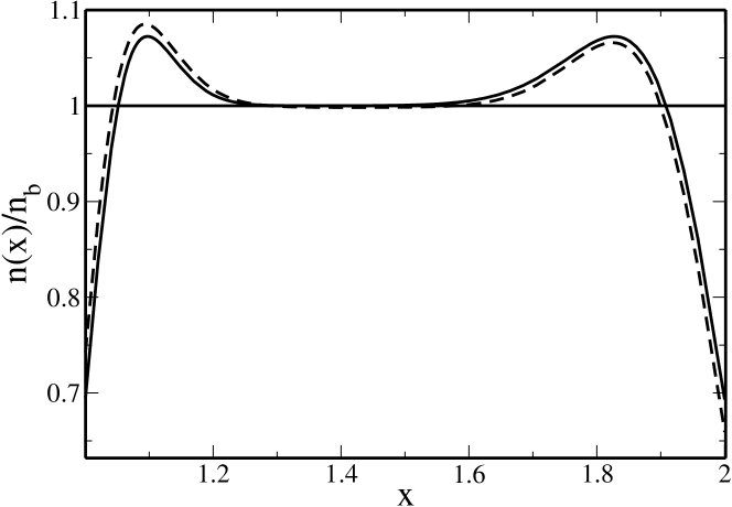
Figure 2: The normalized one-body density $n^{\text{hs}}(x)/n_{b}$, for the 2dOCP on just one universe of the surface ${\cal S}$. The dashed line corresponds to a numerical evaluation, obtained from (85), with $N=100$, $x_{m}=2$ and $\alpha=4.15493$. The full line corresponds to the asymptotic result in the fixed shape limit when $\alpha\to\infty$, and $x_{m}=2$ fixed.

Interestingly, the results (108), (109) and (110) turn out to be the same than the one for a flat space near a hard wall B. Jancovici (1982). From the metric (17), we deduce that the geodesic distance to the boundary at $x_{m}$ is $s=M(x_{m}-x)\sqrt{p^{\prime}(x_{m})/(8x_{m})}$ (when $x_{m}-x$ is of order $1/\sqrt{\alpha}$), and a similar expression for the distance to the boundary at $x=1$ replacing $x_{m}$ by 1. Then, in terms of the geodesic distance $s$ to the border, the results (109) and (110) are exactly the same as those of an OCP in a flat space close to a plane hard wall B. Jancovici (1982),

$$n(s)=\frac{2n_{b}}{\sqrt{\pi}}\int_{0}^{+\infty}\frac{\exp\left[-\left(t-s\sqrt{2\pi n_{b}}\right)^{2}\right]}{1+\mathop{\text{missing}}{erf}(t)}\,dt\,.$$ (111)

This result shows that there exists an interesting universality for the density, because, although we are considering a limit where curvature effects are important, the density turns out to be the same as the one for a flat space.

IV.2 The 2dOCP on the whole surface with potential $-\ln(|z-z^{\prime}|/\sqrt{|zz^{\prime}|})$

IV.2.1 Partition function

Until now we studied the 2dOCP on just one universe. Let us find the thermodynamic properties of the 2dOCP on the whole surface ${\cal S}$. In this case, we also work in the canonical ensemble with a global neutral system. The position $z_{k}=x_{k}e^{i\varphi_{k}}$ of each particle can be in the range $1/x_{m}<x_{k}<x_{m}$. The total number particles $N$ is now expressed in terms of the function $p$ as $N=2\alpha p(x_{m})$. Similar calculations to the ones of the previous section lead to the following expression for the partition function, when $\beta q^{2}=2$,

$$Z^{\mathrm{ws}}=\frac{1}{\lambda^{2N}}Z_{0}^{\mathrm{ws}}\exp(-\beta F_{0}^{\mathrm{ws}})$$ (112)

now, with

$$-\beta F_{0}^{\mathrm{ws}}=Nb_{0}+N\alpha h(x_{m})-\frac{N^{2}}{2}\ln x_{m}-\alpha^{2}\int_{1/x_{m}}^{x_{m}}\frac{\left[p(x)\right]^{2}}{x}\,dx$$ (113)

and

$$Z_{0}^{\mathrm{ws}}=\frac{1}{N!}\int\prod_{i=1}^{N}dS_{i}\,e^{-\alpha h(x_{i})}x_{i}^{-N+1}\prod_{1\leq i<j\leq N}|z_{i}-z_{j}|^{2}\,.$$ (114)

Expanding the Vandermonde determinant and performing the angular integrals we find

$$Z_{0}^{\mathrm{ws}}=\prod_{k=0}^{N-1}\tilde{\mathcal{B}}_{N}(k)$$ (115)

with

$$\tilde{{\cal B}}_{N}(k) = \int x^{2k-N+1}e^{-\alpha h(x)}\,dS$$ (116)

$$= \frac{\alpha}{n}\int_{1/x_{m}}^{x_{m}}x^{2k-N+1}e^{-\alpha h(x)}p^{\prime}(x)\,dx\,.$$ (117)

The function $\tilde{\mathcal{B}}_{N}(k)$ is very similar to $\mathcal{B}_{N}$, and its asymptotic behavior for large values of $N$ can be obtained by Laplace method as explained in appendix B.

IV.2.2 Thermodynamic limit $R\to\infty$, $x_{m}\to\infty$, and fixed $M$

Writing the partition function as

$$\ln Z_{0}^{\mathrm{ws}}=\sum_{k=0}^{N}\ln\tilde{\mathcal{B}}_{N}(k)-\ln\tilde{\mathcal{B}}_{N}(N)\,,$$ (118)

and using the asymptotic expansion (241) for $\tilde{\mathcal{B}}_{N}$, we have

$$\ln Z_{0}^{\mathrm{ws}} = -\ln\frac{n_{b}}{\sqrt{2\pi}}+S_{1}^{\mathrm{ws}}+S_{2}^{\mathrm{ws}}+S_{3}^{\mathrm{ws}}+S_{4}^{\mathrm{ws}}+S_{5}^{\mathrm{ws}}-\ln\left[\sqrt{\alpha}\,x_{m}\left(1+\frac{1}{x_{m}}\right)^{2}\right]$$ (119)

$$-\ln x_{m}-N\ln x_{m}+\alpha h(x_{m})$$

where

$$S_{1}^{\mathrm{ws}} = \sum_{k=0}^{N}\ln\left[\sqrt{\alpha}\,\hat{x}_{k-\frac{N}{2}}\left(1+\frac{1}{\hat{x}_{k-\frac{N}{2}}}\right)^{2}\right]$$ (120)

$$S_{2}^{\mathrm{ws}} = \sum_{k=0}^{N}2\left(k-\frac{N}{2}\right)\ln\hat{x}_{k-\frac{N}{2}}-\alpha h(\hat{x}_{k-\frac{N}{2}})$$ (121)

$$S_{3}^{\mathrm{ws}} = \sum_{k=0}^{N}\ln\frac{\mathop{\text{missing}}{erf}(\epsilon_{k,\min})+\mathop{\text{missing}}{erf}(\epsilon_{k,\max})}{2}$$ (122)

$$S_{4}^{\mathrm{ws}} = \sum_{k=0}^{N}\ln\hat{x}_{k-\frac{N}{2}}$$ (123)

$$S_{5}^{\mathrm{ws}} = \sum_{k^{\prime}=1}^{N/2}\left(\frac{1}{12}+\frac{3}{8}\right)\frac{1}{|k^{\prime}|}+\sum_{k^{\prime}=-N/2}^{-1}\left(\frac{1}{12}-\frac{1}{8}\right)\frac{1}{|k^{\prime}|}=\frac{5}{6}\ln x_{m}+O(1)$$ (124)

and $\epsilon_{k,\min}$ and $\epsilon_{k,\max}$ are defined in equation (243). Notice that $S_{4}^{\text{ws}}=0$ due to the symmetry relation $\hat{x}_{-\ell}=1/\hat{x}_{\ell}$, therefore only the sums $S_{1}^{\text{ws}}$, $S_{2}^{\text{ws}}$, $S_{3}^{\text{ws}}$ and $S_{5}^{\text{ws}}$ contribute to the result. These sums are similar to the ones defined for the half surface case, with the difference that the running index $k^{\prime}=k-N/2$ varies from $-N/2$ to $N/2$ instead of $0$ to $N$ as in the half surface case. This difference is important when considering the remainder terms in the Euler-McLaurin expansion, because now both terms for $k^{\prime}=-N/2$ and $k^{\prime}=N/2$ are important in the thermodynamic limit. In the half surface case only the contribution for $k=N$ was important in the thermodynamic limit.

The asymptotic expansion of each sum, for $x_{m}\to\infty$, is now

$$S_{1}^{\mathrm{ws}} = \frac{N}{2}\ln\alpha+x_{m}^{2}(2\ln x_{m}-1)+2x_{m}(8\ln x_{m}-4)+(28\alpha+1)\ln x_{m}+12\alpha(\ln x_{m})^{2}+O(1)$$

$$S_{2}^{\mathrm{ws}} = \frac{N^{2}}{2}\ln x_{m}+\alpha^{2}\int_{1/x_{m}}^{x_{m}}\frac{\left[p(x)\right]^{2}}{x}\,dx-\alpha Nh(x_{m})+N\ln x_{m}-\alpha h(x_{m})+\frac{1}{3}\ln x_{m}+O(1)$$

$$S_{3}^{\mathrm{ws}} = -2x_{m}\sqrt{\frac{4\pi\alpha}{n_{b}}}\,\beta\gamma_{\text{hard}}+O(1)$$ (127)

where $\gamma$ is defined in equation (72). The free energy is given by $\beta F^{\mathrm{ws}}=-\ln Z^{\mathrm{ws}}$, with

$$\ln Z^{\mathrm{ws}} = 2\alpha x_{m}^{2}\ln x_{m}+N\left(b_{0}+\ln\frac{\sqrt{2\pi\alpha}}{\lambda^{2}n_{b}}\right)-\alpha x_{m}^{2}+8\alpha x_{m}(2\ln x_{m}-1)-2\mathcal{C}_{R}\,\beta\gamma_{\text{hard}}$$ (128)

$$+12\alpha(\ln x_{m})^{2}+28\alpha\ln x_{m}+\frac{1}{6}\ln x_{m}+O(1)\,.$$

We notice that the free energy for this system turns out to be nonextensive with a term $2x_{m}^{2}\ln x_{m}$. This is probably due to the special form of the potential $-\ln(|z-z^{\prime}|/\sqrt{|zz^{\prime}|})$: the contribution from the denominator in the logarithm can be written as a one-body term $[(N-1)/2]\ln x$, which is not intensive but extensive. However, this nonextensivity of the final result is mild, and can be cured by choosing the arbitrary additive constant $b_{0}$ of the Coulomb potential as $b_{0}=-\ln(Mx_{m})+\text{constant}$.

IV.2.3 Thermodynamic limit at fixed shape: $\alpha\to\infty$ and $x_{m}$ fixed

For this situation, we use the asymptotic behavior (244) of $\tilde{\mathcal{B}}_{N}$

$$\ln Z_{0}^{\mathrm{ws}}=N\ln\frac{\sqrt{\pi\alpha}}{n_{b}}+S_{1}^{\mathrm{ws,fixed}}+S_{2}^{\mathrm{ws,fixed}}+S_{3}^{\mathrm{ws,fixed}}+S_{4}^{\mathrm{ws,fixed}}$$ (129)

where, now

$$S_{1}^{\mathrm{ws,fixed}} = \frac{1}{2}\sum_{k=0}^{N-1}\ln[\hat{x}_{k-\frac{N}{2}}p^{\prime}(\hat{x}_{k-\frac{N}{2}})]$$ (130)

$$S_{2}^{\mathrm{ws,fixed}} = -\alpha\sum_{k=0}^{N-1}[h(\hat{x}_{k-\frac{N}{2}})-2p(\hat{x}_{k-\frac{N}{2}})\ln\hat{x}_{k-\frac{N}{2}}]$$ (131)

$$S_{3}^{\mathrm{ws,fixed}} = \sum_{k=0}^{N-1}\ln\frac{\mathop{\text{missing}}{erf}(\epsilon_{k,\min})+\mathop{\text{missing}}{erf}(\epsilon_{k,\max})}{2}$$ (132)

$$S_{4}^{\mathrm{ws,fixed}} = \sum_{k=0}^{N-1}\ln\hat{x}_{k-\frac{N}{2}}$$ (133)

These sums can be computed as earlier using Euler-McLaurin summation formula. We notice that

$$S_{4}^{\mathrm{ws,fixed}}=\alpha\int_{1/x_{m}}^{x_{m}}\ln x\,p^{\prime}(x)\,dx+O(1)=0+O(1)$$ (134)

because of the symmetry properties $\ln(1/x)=-\ln x$ and $p^{\prime}(1/x)d(1/x)=-p^{\prime}(x)dx$. In the computation of $S_{2}^{\mathrm{ws,fixed}}$ there is an important difference with the case of the half surface section, due to the contribution when $k=0$, since $\hat{x}_{-N/2}=1/\hat{x}_{N/2}=1/x_{m}$

$$S_{2}^{\mathrm{ws,fixed}}=-\alpha Nh(x_{m})-\frac{N^{2}}{2}\ln x_{m}+\alpha^{2}\int_{1/x_{m}}^{x_{m}}\frac{\left[p(x)\right]^{2}}{x}\,dx+O(1)\,.$$ (135)

There is no $O(\alpha)$ contribution from $S_{2}^{\mathrm{ws,fixed}}$. Finally, the free energy $\beta F^{\mathrm{ws}}=-\ln Z^{\mathrm{ws}}$ is given by

$$\ln Z^{\mathrm{ws}} = \alpha\left[-2p(x_{m})\left(\ln\frac{\sqrt{2\pi\alpha}}{\lambda^{2}n_{b}}+b_{0}\right)+\int_{1/x_{m}}^{x_{m}}\frac{(1+x)^{4}}{x^{3}}\,\ln\frac{(x+1)^{4}}{x^{2}}\,dx\right]$$ (136)

$$-2\sqrt{\frac{4\pi\alpha}{n_{b}}}\,x_{m}\left(1+\frac{1}{x_{m}}\right)^{2}\beta\gamma_{\text{hard}}+O(1)$$

We notice that the free energy has again a nonextensive term proportional to $\alpha\ln{\alpha}$, but, once again, it can be cured by choosing the constant $b_{0}$ as $b_{0}=-\ln(Mx_{m})+\text{constant}$. The perimeter correction, $2\mathcal{C}_{R}\beta\gamma_{\text{hard}}$, proportional to $\sqrt{\alpha}$, has the same form as for the half surface case, with equal contributions from each boundary at $x=1/x_{m}$ and $x=x_{m}$. Once again, there is no $\ln\alpha$ correction in agreement with the general theory of Ref. B. Jancovici, G. Manificat, and C. Pisani (1994); B. Jancovici and G. Téllez (1996) and the fact that the Euler characteristic of this manifold is $\chi=0$.

IV.2.4 Density

The density is now given by

$$n^{\mathrm{ws}}(x)=\sum_{k=0}^{N-1}\frac{x^{2k-N+1}\,e^{-\alpha h(x)}}{\tilde{\mathcal{B}}_{N}(k)}$$ (137)

Due to the fact that the asymptotic behavior of $\tilde{\mathcal{B}}_{N}(k)$ is almost the same as the one of $\mathcal{B}_{N}(k^{\prime})$ with $k^{\prime}=|k-\frac{N}{2}|$, the behavior of the density turn out to be the same as for the half surface case, in the thermodynamic limit $\alpha\to\infty$, $x_{m}$ fixed,

$$n(x)=n_{b}\,,\qquad\text{in the bulk, ie., when $x-x_{m}$ and $x-\frac{1}{x_{m}}$ are of order 1.}$$ (138)

And, close to the boundaries, $x\to x_{b}$ with $x_{b}=x_{m}$ or $x_{b}=1/x_{m}$,

$$n(x)=\frac{2n_{b}}{\sqrt{\pi}}\int_{0}^{+\infty}\frac{\exp\left[-\left(t-\sqrt{\frac{\alpha p^{\prime}(x_{b})}{x_{b}}}|x-x_{b}|)\right)^{2}\right]}{1+\mathop{\text{missing}}{erf}(t)}\,dt\,,\quad\text{for $x_{b}-x$ of order }\frac{1}{\sqrt{\alpha}}\,.$$ (139)

If the result is expressed in terms of the geodesic distance $s$ to the border, we recover, once again, the result of the OCP in a flat space near a hard wall (111).

IV.3 The 2dOCP on the half surface with potential $-\ln(|z-z^{\prime}|/\sqrt{|zz^{\prime}|})$

IV.3.1 Partition function

In this case, we have $N=\alpha p(x_{m})$. Following similar calculations to the ones of the previous cases, we find that the partition function, at $\beta q^{2}=2$, is

$$Z^{\overline{\mathrm{hs}}}=Z_{0}^{\overline{\mathrm{hs}}}e^{-\beta F_{0}^{\overline{\mathrm{hs}}}}$$ (140)

with

$$-\beta F_{0}^{\overline{\mathrm{hs}}}=\alpha^{2}p(x_{m})h(x_{m})-p(x_{m})^{2}\ln x_{m}+\int_{1}^{x_{m}}\frac{\left[p(x)\right]^{2}}{x}\,dx-Nb_{0}$$ (141)

and

$$Z_{0}^{\overline{\mathrm{hs}}}=\prod_{k=0}^{N-1}\hat{\mathcal{B}}_{N}(k)$$ (142)

with

$$\hat{\mathcal{B}}_{N}(k)=\frac{\alpha}{n_{b}}\int_{1}^{x_{m}}x^{2k+1}e^{-\alpha h(x)}\,dx$$ (143)

IV.3.2 Thermodynamic limit $R\to\infty$, $x_{m}\to\infty$, and fixed $M$

The asymptotic expansion of $\hat{\mathcal{B}}_{N}(k)$ is obtained from equation (241) replacing $k^{\prime}$ by $k$ and considering only the case $k>0$. As explained in appendix B, the main difference with the other half surface case (section IV.1), is an additional term $\hat{x}_{k}$ in each factor of the partition function and the additional term $(3/(8k))$ in the expansion (241). Therefore, the partition function can be obtained from the one of the half surface with potential $-\ln|z-z^{\prime}|$ by adding the terms

$$S_{4}^{\overline{\mathrm{hs}}} = \sum_{k=0}^{N-1}\ln\hat{x}_{k}\,,$$ (144)

$$S_{5}^{\overline{\mathrm{hs}}} = \sum_{k=1}^{N-1}\frac{3}{8k}=\frac{3}{8}\ln N+O(1)=\frac{3}{4}\ln x_{m}+O(1)\,.$$ (145)

Using Euler-McLaurin expansion, we have

$$S_{4}^{\overline{\mathrm{hs}}} = \sum_{k=0}^{N}\ln\hat{x}_{k}-\ln x_{m}$$ (146)

$$= \int_{1}^{x_{m}}\alpha p^{\prime}(x)\ln x\,dx+\frac{1}{2}\ln x_{m}-\ln x_{m}+O(1)$$

$$= \alpha p(x_{m})\ln x_{m}-\alpha\int_{1}^{x_{m}}\frac{p(x)}{x}\,dx-\frac{1}{2}\ln x_{m}+O(1)$$

$$= \alpha p(x_{m})\ln x_{m}-\frac{1}{2}\alpha h(x_{m})-\frac{1}{2}\ln x_{m}+O(1)\,,$$

where we used the property (41). Finally,

$$\ln Z^{\overline{\mathrm{hs}}} = \alpha x_{m}^{2}\ln x_{m}+N\left(b_{0}+\ln\frac{\sqrt{2\pi\alpha}}{\lambda^{2}n_{b}}\right)-\frac{\alpha}{2}x_{m}^{2}+4\alpha x_{m}(2\ln x_{m}-1)$$ (147)

$$-\mathcal{C}_{R}\,\beta\gamma_{\text{hard}}+6\alpha(\ln x_{m})^{2}+14\alpha\ln x_{m}+\frac{1}{12}\ln x_{m}+O(1)\,.$$

The result is one-half of the one for the full surface, $\ln Z^{\mathrm{ws}}$, as it might be expected.

IV.3.3 Thermodynamic limit at fixed shape: $\alpha\to\infty$ and $x_{m}$ fixed

For this case, the asymptotics of $\hat{\mathcal{B}}_{N}$ are very similar to those of $\mathcal{B}_{N}$ from equation (228)

$$\hat{\mathcal{B}}_{N}(k)\sim\hat{x}_{k}\mathcal{B}_{N}(k)\,.$$ (148)

Therefore, the only difference from the calculations of the half surface case with potential $-\ln|z-z^{\prime}|+\text{constant}$, and this case, is the sum

$$S_{4}^{\overline{\mathrm{hs}},\mathrm{fixed}}=\sum_{k=0}^{N-1}\ln\hat{x}_{k}\,.$$ (149)

We have

$$S_{4}^{\overline{\mathrm{hs}},\mathrm{fixed}} = \int_{1}^{x_{m}}\alpha p^{\prime}(x)\ln x\,dx+O(1)$$ (150)

$$= \alpha p(x_{m})\ln x_{m}-\frac{1}{2}\alpha h(x_{m})+O(1)\,.$$

Here, the term $k=N$ and the remainder of the Euler-McLaurin expansion give corrections of order $O(\alpha^{0})=O(1)$, as opposed to the previous section where they gave contributions of order $O(\ln x_{m})$.

Finally, we find

$$\ln Z^{\overline{\mathrm{hs}}} = \alpha\left[p(x_{m})\left(\frac{1}{2}\ln\frac{\sqrt{2\alpha\pi}}{n_{b}}+b_{0}\right)+\int_{1}^{\infty}\frac{(1+x)^{4}}{x^{3}}\ln\frac{(1+x)^{4}}{x^{2}}\,dx\right]$$ (151)

$$-\sqrt{\frac{4\pi\alpha}{n_{b}}}\left[x_{m}\left(1+\frac{1}{x_{m}}\right)+4\right]\beta\gamma_{\text{hard}}+O(1)\,.$$

The bulk free energy, proportional to $\alpha$, plus the nonextensive term proportional $\alpha\ln\alpha$, are one-half the ones from equation (136) for the full surface case, as expected. The perimeter contribution, proportional to $\sqrt{\alpha}$ is again the same as in all the previous cases of thermodynamic limit at fixed shape, i.e. a contribution $\beta\gamma_{\text{hard}}\mathcal{C}_{b}$ for each boundary at $x_{b}=x_{m}$ and at $x_{b}=1$ with perimeter $\mathcal{C}_{b}$ (82). Once again, there is no $\ln\alpha$ correction in agreement with the fact that the Euler characteristic of this manifold is $\chi=0$.

IV.4 The grounded horizon case

IV.4.1 Grand canonical partition function

In order to find the partition function for the system in the half space, with a metallic grounded boundary at $x=1$, when the charges interacting through the pair potential of Eq. (33) it is convenient to work in the grand canonical ensemble instead, and use the techniques developed in Refs. P. J. Forrester (1985); B. Jancovici and G. Téllez (1996). We consider a system with a fixed background density $\rho_{b}$. The fugacity $\tilde{\zeta}=e^{\beta\mu}/\lambda^{2}$, where $\mu$ is the chemical potential, controls the average number of particles $\langle N\rangle$, and in general the system is nonneutral $\langle N\rangle\neq N_{b}$, where $N_{b}=\alpha p(x_{m})$. The excess charge is expected to be found near the boundaries at $x=1$ and $x=x_{m}$, while in the bulk the system is expected to be locally neutral. In order to avoid the collapse of a particle into the metallic boundary, due to its attraction to the image charges, we confine the particles to be in a “disk” domain $\tilde{\Omega}_{R}$, where $x\in[1+w,x_{m}]$. We introduced a small gap $w$ between the metallic boundary and the domain containing the particles, the geodesic width of this gap is $W=\sqrt{\alpha p^{\prime}(1)/(2\pi n_{b})}\,w$. On the other hand, for simplicity, we consider that the fixed background extends up to the metallic boundary.

In the potential energy of the system (45) we should add the self energy of each particle, that is due to the fact that each particle polarizes the metallic boundary, creating an induced surface charge density. This self energy is $\frac{q^{2}}{2}\ln[|x^{2}-1|M/2L]$, where the constant $\ln(M/2L)$ has been added to recover, in the limit $M\to 0$, the self energy of a charged particle near a plane grounded wall in flat space.

The grand partition function, when $\beta q^{2}=2$, is

$$\Xi=e^{-\beta F_{0}^{\text{gh}}}\left[1+\sum_{N=1}^{\infty}\frac{\zeta^{N}}{N!}\int\prod_{i=1}^{N}dS_{i}\prod_{i<j}\left|\frac{z_{i}-z_{j}}{1-z_{i}\bar{z}_{j}}\right|^{2}\prod_{i=1}^{N}\left||z_{i}|^{2}-1\right|^{-1}\prod_{i=1}^{N}e^{-\alpha[h(x_{i})-2N_{b}\ln x_{i}]}\right]$$ (152)

where for $N=1$ the product $\prod_{i<j}$ must be replaced by 1. The domain of integration for each particle is $\tilde{\Omega}_{R}$. We have defined a rescaled fugacity $\zeta=2L\tilde{\zeta}/M$ and

$$-\beta F_{0}^{\text{gh}}=\alpha N_{b}h(x_{m})-N_{b}^{2}\ln x_{m}-\alpha^{2}\int_{1}^{x_{m}}\frac{[p(x)]^{2}}{x}\,dx$$ (153)

which is very similar to $F_{0}^{\text{hs}}$, except that here $N_{b}=\alpha p(x_{m})$ is not equal to $N$ the number of particles.

Let us define a set of reduced complex coordinates $u_{i}=z_{i}$ and its corresponding images $u_{i}^{*}=1/\bar{z}_{i}$. By using Cauchy identity

$$\det\left(\frac{1}{u_{i}-u_{j}^{*}}\right)_{(i,j)\in\{1,\cdots,N\}^{2}}=(-1)^{N(N-1)/2}\>\frac{\prod_{i<j}(u_{i}-u_{j})(u^{*}_{i}-u^{*}_{j})}{\prod_{i,j}(u_{i}-u_{j}^{*})}$$ (154)

the particle-particle interaction and self energy terms can be cast into the form

$$\prod_{i<j}\left|\frac{z_{i}-z_{j}}{1-z_{i}\bar{z}_{j}}\right|^{2}\prod_{i=1}^{N}\left(|z_{i}|^{2}-1\right)^{-1}=(-1)^{N}\det\left(\frac{1}{1-z_{i}\bar{z}_{j}}\right)_{(i,j)\in\{1,\cdots,N\}^{2}}\,.$$ (155)

The grand canonical partition function is then

$$\Xi=e^{-\beta F_{0}^{\text{gh}}}\left[1+\sum_{N=1}^{\infty}\frac{1}{N!}\int\prod_{i=1}^{N}dS_{i}\prod_{i=1}^{N}\left[-\zeta(x_{i})\right]\,\det\left(\frac{1}{1-z_{i}\bar{z}_{j}}\right)\right]\,,$$ (156)

with $\zeta(x)=\zeta e^{-\alpha[h(x)-2N_{b}\ln x]}$. We shall now recall how this expression can be reduced to a Fredholm determinant P. J. Forrester (1985). Let us consider the Gaussian partition function

$$Z_{0}=\int{\cal D}\psi{\cal D}\bar{\psi}\,\exp\left[\int\bar{\psi}({\bf q})A^{-1}(z,\bar{z}^{\prime})\psi({\bf q}^{\prime})\,dS\,dS^{\prime}\right]\,.$$ (157)

The fields $\psi$ and $\bar{\psi}$ are anticommuting Grassmann variables. The Gaussian measure in (157) is chosen such that its covariance is equal to

$$\left<\bar{\psi}({\bf q}_{i})\psi({\bf q}_{j})\right>=A(z_{i},\bar{z}_{j})=\frac{1}{1-z_{i}\bar{z}_{j}}$$ (158)

where $\langle\ldots\rangle$ denotes an average taken with the Gaussian weight of (157). By construction we have

$$Z_{0}=\det(A^{-1})$$ (159)

Let us now consider the following partition function

$$Z=\int{\cal D}\psi{\cal D}\bar{\psi}\exp\left[\int\bar{\psi}({\bf q})A^{-1}(z,\bar{z}^{\prime})\psi({\bf q}^{\prime})dSdS^{\prime}-\int\zeta(x)\bar{\psi}({\bf q})\psi({\bf q})\,dS\right]$$ (160)

which is equal to

$$Z=\det(A^{-1}-\zeta)$$ (161)

and then

$$\frac{Z}{Z_{0}}=\det[A(A^{-1}-\zeta)]=\det(1+K)$$ (162)

where $K$ is an integral operator (with integration measure $dS$) with kernel

$$K({\bf q},{\bf q}^{\prime})=-\zeta(x^{\prime})\,A(z,\bar{z}^{\prime})=-\frac{\zeta(x^{\prime})}{1-z\bar{z}^{\prime}}\,.$$ (163)

Expanding the ratio $Z/Z_{0}$ in powers of $\zeta$ we have

$$\frac{Z}{Z_{0}}=1+\sum_{N=1}^{\infty}\frac{1}{N!}\int\prod_{i=1}^{N}dS_{i}(-1)^{N}\prod_{i=1}^{N}\zeta(x_{i})\left<\bar{\psi}({\bf q}_{1})\psi({\bf q}_{1})\cdots\bar{\psi}({\bf q}_{N})\psi({\bf q}_{N})\right>$$ (164)

Now, using Wick theorem for anticommuting variables Zinn-Justin (1993), we find that

$$\left<\bar{\psi}({\bf q}_{1})\psi({\bf q}_{1})\cdots\bar{\psi}({\bf q}_{N})\psi({\bf q}_{N})\right>=\det A(z_{i},\bar{z}_{j})=\det\left(\frac{1}{1-z_{i}\bar{z}_{j}}\right)$$ (165)

Comparing equations (164) and (156) with the help of equation (165) we conclude that

$$\Xi=e^{-\beta F_{0}^{\text{gh}}}\,\frac{Z}{Z_{0}}=e^{-\beta F_{0}^{\text{gh}}}\det(1+K)$$ (166)

The problem of computing the grand canonical partition function has been reduced to finding the eigenvalues $\lambda$ of the operator $K$. The eigenvalue problem for $K$ reads

$$-\int_{\tilde{\Omega}_{R}}\frac{\zeta(x^{\prime})}{1-z\bar{z}^{\prime}}\,\Phi(x^{\prime},\varphi^{\prime})dS^{\prime}=\lambda\Phi(x,\varphi)$$ (167)

For $\lambda\neq 0$ we notice from equation (167) that $\Phi(x,\varphi)=\Phi(z)$ is an analytical function of $z=xe^{i\varphi}$ in the region $|z|>1$. Because of the circular symmetry, it is natural to try $\Phi(z)=\Phi_{\ell}(z)=z^{-\ell}$ with $\ell\geq 1$ a positive integer. Expanding

$$\frac{1}{1-z\bar{z}^{\prime}}=-\sum_{n=1}^{\infty}\left(z\bar{z}^{\prime}\right)^{-n}$$ (168)

and replacing $\Phi_{\ell}(z)=z^{-\ell}$ in equation (167), we show that $\Phi_{\ell}$ is indeed an eigenfunction of $K$ with eigenvalue

$$\lambda_{\ell}=\zeta\mathcal{B}_{N_{b}}^{\text{gh}}(N_{b}-\ell)$$ (169)

where

$$\mathcal{B}_{N_{b}}^{\text{gh}}(k)=\frac{\alpha}{n_{b}}\int_{1+w}^{x_{m}}x^{2k}e^{-\alpha h(x)}\,p^{\prime}(x)\,dx$$ (170)

which is very similar to $\mathcal{B}_{N}$ defined in Eq. (55), except for the small gap $w$ in the lower limit of integration. So, we arrive to the result for the grand potential

$$\beta\Omega=-\ln\Xi=\beta F_{0}^{\text{gh}}-\sum_{\ell=1}^{\infty}\ln\left[1+\zeta{\cal B}_{N_{b}}^{\text{gh}}(N_{b}-\ell)\right]\,.$$ (171)

IV.4.2 Thermodynamic limit at fixed shape: $\alpha\to\infty$ and $x_{m}$ fixed

Let us define $k=N_{b}-\ell$ for $\ell\in\mathbb{N}^{*}$, thus $k$ is positive, then negative when $\ell$ increases. Therefore, it is convenient to split the sum (171) in $\ln\Xi$ into two parts

$$S_{6}^{\text{gh,fixed}} = \sum_{k=-\infty}^{-1}\ln[1+\zeta\mathcal{B}_{N_{b}}^{\text{gh}}(k)]$$ (172)

$$S_{7}^{\text{gh,fixed}} = \sum_{k=0}^{N_{b}-1}\ln[1+\zeta\mathcal{B}_{N_{b}}^{\text{gh}}(k)]\,.$$ (173)

The asymptotic behavior of $\mathcal{B}_{N_{b}}^{\text{gh}}(k)$ when $\alpha\to\infty$ can be directly deduced from the one of $\mathcal{B}_{N}$ found in appendix B, Eq. (228), taking into account the small gap $w$ near the boundary at $x=1+w$. When $k<0$, we have $\hat{x}_{k}<1$, then we notice that $\epsilon_{k,1}$ defined in (230) is negative, and that the relevant contributions to the sum $S_{6}^{\text{gh,fixed}}$ are obtained when $k$ is close to 0, more precisely $k$ of order $O(\sqrt{N_{b}})$. So, we expand $\hat{x}_{k}$ around $\hat{x}_{k}=1$ up to order $(\hat{x}_{k}-1)^{2}$ in the exponential term $e^{-\alpha[h(\hat{x}_{k})-2p(\hat{x}_{k})\ln\hat{x}_{k}]}$ from Eq. (228). Then, we have, for $k<0$ of order $O(\sqrt{N_{b}})$,

$$\mathcal{B}_{N_{b}}^{\text{gh}}(k)=\frac{\sqrt{\alpha\pi p^{\prime}(1)}}{2n_{b}}e^{\alpha p^{\prime}(1)\,(1-\hat{x}_{k})^{2}}\mathop{\text{missing}}{erfc}[\sqrt{\alpha p^{\prime}(1)}\,(1+w-\hat{x}_{k})]$$ (174)

where $\mathop{\text{missing}}{erfc}(u)=1-\mathop{\text{missing}}{erf}(u)$ is the complementary error function. Then, up to corrections of order $O(1)$, the sum $S_{6}^{\text{gh,fixed}}$ can be transformed into an integral over the variable $t=\sqrt{\alpha p^{\prime}(1)}\,(1-\hat{x}_{k})$, to find

$$S_{6}^{\text{gh,fixed}}=\sqrt{\alpha p^{\prime}(1)}\int_{0}^{\infty}\ln\left[1+\frac{\zeta\sqrt{\alpha\pi p^{\prime}(1)}}{2n_{b}}e^{t^{2}}\,\mathop{\text{missing}}{erfc}\left(t+\sqrt{2\pi n_{b}}W\right)\right]\,dt+O(1)\,.$$ (175)

Let $\mathcal{C}_{1}=\sqrt{2\pi\alpha p^{\prime}(1)/n_{b}}$, be total length of the boundary at $x=1$. We notice that

$$\zeta\frac{\sqrt{\alpha\pi p^{\prime}(1)}}{2n_{b}}=\frac{\zeta\mathcal{C}_{1}}{\sqrt{2n_{b}}}=\frac{2\tilde{\zeta}L}{\sqrt{2n_{b}}}\frac{\mathcal{C}_{1}}{M}$$ (176)

is fixed and of order $O(1)$ in the limit $M\to\infty$, since in the fixed shape limit $\mathcal{C}_{1}/M$ is fixed. Therefore $S_{6}^{\text{gh,fixed}}$ gives a contribution proportional to the perimeter $\mathcal{C}_{1}$.

For $S_{7}^{\text{gh,fixed}}$, we define

$$\tilde{\epsilon}_{k,1}=\sqrt{\alpha p^{\prime}(1)}\,(1+w-\hat{x}_{k})\,,$$ (177)

and we write

$$S_{7}^{\text{gh,fixed}} = \sum_{k=0}^{N_{b}-1}\ln\left[1+\frac{\zeta\sqrt{\alpha\pi\hat{x}_{k}p^{\prime}(\hat{x}_{k})}}{2n_{b}}e^{-\alpha[h(\hat{x}_{k})-2p(\hat{x}_{k})\ln\hat{x}_{k}]}\left[\mathop{\text{missing}}{erf}(\tilde{\epsilon}_{k,1})+\mathop{\text{missing}}{erf}({\epsilon}_{k,m})\right]\right]$$ (178)

$$= S_{8}^{\text{gh,fixed}}+S_{1}^{\text{hs,fixed}}+S_{2}^{\text{hs,fixed}}+N_{b}\ln\frac{\zeta\sqrt{\alpha\pi}}{n_{b}}$$

where

$$S_{8}^{\text{gh,fixed}}=\sum_{k=0}^{N_{b}-1}\ln\left[\frac{n_{b}e^{\alpha[h(\hat{x}_{k})-2p(\hat{x}_{k})\ln\hat{x}_{k}]}}{\zeta\sqrt{\alpha\pi\hat{x}_{k}p^{\prime}(\hat{x}_{k})}}+\frac{1}{2}\left[\mathop{\text{missing}}{erf}(\tilde{\epsilon}_{k,1})+\mathop{\text{missing}}{erf}(\epsilon_{k,m})\right]\right]$$ (179)

and we see that the sums $S_{1}^{\text{hs,fixed}}$ and $S_{2}^{\text{hs,fixed}}$ reappear. These are defined in equations (75) and (76) and computed in (78) and (79). In a similar way to $S_{6}^{\text{gh,fixed}}$, $S_{8}^{\text{gh,fixed}}$ gives only boundary contributions when $k$ is close to 0, of order $\sqrt{N_{b}}$ (grounded boundary at $x=1$) and when $k$ is close to $N_{b}$ with $N_{b}-k$ of order $\sqrt{N_{b}}$ (boundary at $x=x_{m}$). We have,

$$S_{8}^{\text{gh,fixed}} = \sqrt{\alpha p^{\prime}(1)}\int_{0}^{\infty}\ln\left[\frac{n_{b}e^{-t^{2}}}{\zeta\sqrt{\alpha\pi p^{\prime}(1)}}+\frac{1}{2}\left[\mathop{\text{missing}}{erf}(t-\sqrt{2\pi n_{b}}W)+1\right]\right]\,dt$$ (180)

$$+\sqrt{\alpha x_{m}p^{\prime}(x_{m})}\int_{0}^{\infty}\ln\left[\frac{\mathop{\text{missing}}{erf}(t)+1}{2}\right]\,dt$$

Let us introduce again the perimeter of the outer boundary at $x=x_{m}$, $\mathcal{C}_{R}=\sqrt{2\pi\alpha x_{m}p^{\prime}(x_{m})/n_{b}}$. Putting together all terms, we finally have

$$\ln\Xi = -N_{b}\beta\omega_{B}+\frac{\alpha}{2}\left[h(x_{m})-2p(x_{m})\ln x_{m}\right]+\alpha\int_{1}^{x_{m}}\frac{(1+x)^{4}}{x^{3}}\ln\frac{(1+x)^{4}}{x^{2}}\,dx$$ (181)

$$-\mathcal{C}_{1}\beta\gamma_{\text{metal}}-\mathcal{C}_{R}\beta\gamma_{\text{hard}}+O(1)$$

where

$$\beta\omega_{B}=-\ln\frac{2\pi\tilde{\zeta}L}{\sqrt{2n_{b}}}$$ (182)

is the bulk grand potential per particle of the OCP near a plane metallic wall in the flat space. The surface (perimeter) tensions $\gamma_{\text{metal}}$ and $\gamma_{\text{hard}}$ associated to each boundary (metallic at $x_{b}=1$, and hard wall at $x_{b}=x_{m}$) are given by

$$\beta\gamma_{\text{metal}} = -\sqrt{\frac{n_{b}}{2\pi}}\int_{0}^{\infty}\ln\left[1+\frac{\zeta\sqrt{\alpha\pi x_{b}p^{\prime}(x_{b})}}{2n_{b}}e^{t^{2}}\,\mathop{\text{missing}}{erfc}\left(t+\sqrt{2\pi n_{b}}W\right)\right]\,dt$$ (183)

$$-\sqrt{\frac{n_{b}}{2\pi}}\int_{0}^{\infty}\ln\left[\frac{n_{b}e^{-t^{2}}}{\zeta\sqrt{\alpha\pi p^{\prime}(x_{b})x_{b}}}+\frac{1}{2}\left[\mathop{\text{missing}}{erf}(t-\sqrt{2\pi n_{b}}W)+1\right]\right]\,dt$$

with $x_{b}=1$, and (72) for $\beta\gamma_{\text{hard}}$.

Notice, once again, that the combination

$$\frac{\zeta\sqrt{\alpha\pi x_{b}p^{\prime}(x_{b})}}{2n_{b}}=\frac{2\tilde{\zeta}L}{\sqrt{2n_{b}}}\frac{\mathcal{C}_{b}}{M}$$ (184)

is finite in this fixed shape limit, since the perimeter $\mathcal{C}_{b}$ of the boundary at $x_{b}$ scales as $M$. Up to a rescaling of the fugacity $\tilde{\zeta}$ to absorb the factor $\mathcal{C}_{b}/M$, the surface tension near the metallic boundary $\gamma_{\text{metal}}$ is the same as the one found in Ref. B. Jancovici and G. Téllez (1996) in flat space. It is also similar to the one found in Ref. P. J. Forrester (1985) with a small difference due to the fact that in that reference the background does not extend up to the metallic boundary, but has also a small gap near the boundary.

There is no $\ln\alpha$ correction in the grand potential in agreement with the fact that the Euler characteristic of the manifold is $\chi=0$.

Let us decompose $\ln\Xi$ into its bulk and perimeter parts,

$$\ln\Xi=-\beta\Omega_{b}^{\text{gh}}-\mathcal{C}_{1}\beta\gamma_{\text{metal}}-\mathcal{C}_{R}\beta\gamma_{\text{hard}}+O(1)$$ (185)

with the bulk grand potential $\Omega_{b}^{\text{gh}}$ given by

$$-\beta\Omega_{b}^{\text{gh}}=-N_{b}\beta\omega_{B}+\frac{\alpha}{2}\left[h(x_{m})-2p(x_{m})\ln x_{m}\right]+\alpha\int_{1}^{x_{m}}\frac{(1+x)^{4}}{x^{3}}\ln\frac{(1+x)^{4}}{x^{2}}\,dx\,.$$ (186)

The average number of particles is given by the usual thermodynamic relation $\langle N\rangle=\zeta\partial(\ln\Xi)/\partial\zeta$. Following (185), it can be decomposed into bulk and perimeter contributions,

$$\langle N\rangle=N_{b}-\mathcal{C}_{1}\zeta\frac{\partial\beta\gamma_{\text{metal}}}{\partial\zeta}\,.$$ (187)

The boundary at $x=x_{m}$ does not contribute because $\gamma_{\text{hard}}$ does not depend on the fugacity. From this equation, we can deduce the perimeter linear charge density $\sigma$ which accumulates near the metallic boundary

$$\sigma=-\zeta\frac{\partial\beta\gamma_{\text{metal}}}{\partial\zeta}\,.$$ (188)

We can also notice that the bulk Helmoltz free energy $F_{b}^{\text{gh}}=\Omega_{b}^{\text{gh}}+\mu N_{b}$ is the same as for the half surface, with Coulomb potential $G^{\text{hs}}$, given in (81).

IV.4.3 Thermodynamic limit $R\to\infty$, $x_{m}\to\infty$, and fixed $M$

This limit is of restricted interest, since the metallic boundary perimeter remains of order $O(1)$, we expect to find the same thermodynamic quantities as in the half surface case with hard wall “horizon” boundary up to order $O(\ln x_{m})$. This is indeed the case: let us split $\ln\Xi$ into two sums $S_{6}^{\text{gh}}$ and $S_{7}^{\text{gh}}$ as in (172) and (173). For $k<0$, the asymptotic expansion of $\mathcal{B}_{N_{b}}(k)$ derived in appendix B should be revised, because the absolute maximum of the integrand is obtained for values of the variable of integration outside the domain of integration. Within the domain of integration the maximum value of the integrand in (170) is obtained when $x=1+w$. Expanding the integrand around that value, we obtain to first order, for large $|k|$,

$$\mathcal{B}_{N_{b}}^{\text{gh}}(k)\sim\frac{\alpha p^{\prime}(1+w)}{2n_{b}|k|}e^{-2w|k|}\,.$$ (189)

Then

$$S_{6}^{\text{gh}} = \sum_{k=-\infty}^{0}\ln\left[1+\zeta\mathcal{B}_{N_{b}}^{\text{gh}}(k)\right]$$ (190)

$$= \int_{0}^{\infty}dk\ln\left[1+\zeta\frac{\alpha p^{\prime}(1+w)}{2n_{b}|k|}e^{-2w|k|}\right]+O(1)$$

$$= O(1)\,,$$

does not contribute to the result at orders greater than $O(1)$. For the other sum, we have

$$S_{7}^{\text{gh}} = \sum_{k=0}^{N_{b}}\ln\left[\zeta\mathcal{B}_{N_{b}}^{\text{gh}}(k)\right]+\sum_{k=0}^{N_{b}}\ln\left[1+\frac{1}{\zeta\mathcal{B}_{N_{b}}^{\text{gh}}(k)}\right]$$ (191)

$$= \sum_{k=0}^{N_{b}}\ln\left[\zeta\mathcal{B}_{N_{b}}^{\text{gh}}(k)\right]+O(1)\,.$$

The second sum is indeed $O(1)$, because $1/[\zeta\mathcal{B}_{N_{b}}^{\text{gh}}(k)]$ has a fast exponential decay for large $k$, therefore the sum can be converted into an finite [order $O(1)$] integral over the variable $k$.

Now, since the asymptotic behavior of $\mathcal{B}_{N_{b}}^{\text{gh}}(k)$, for $k>0$ and large, is essentially the same as the one for $\mathcal{B}_{N_{b}}(k)$, we immediately find, up to $O(1)$ corrections,

$$\ln\Xi=\beta\mu N_{b}+\ln Z^{\text{hs}}+O(1)$$ (192)

where $\ln Z^{\text{hs}}$ is minus the free energy in the half surface case with hard wall boundary, given by (70).

IV.4.4 The one-body density

As usual one can compute the density by doing a functional derivative of the grand potential with respect to a position-dependent fugacity $\zeta({\bf q})$

$$n^{\text{gh}}({\bf q})=\zeta({\bf q})\frac{\delta\ln\Xi}{\delta\zeta({\bf q})}\,.$$ (193)

For the present case of a curved space, we shall understand the functional derivative with the rule $\frac{\delta\zeta({\bf q}^{\prime})}{\delta\zeta({\bf q})}=\delta({\bf q},{\bf q}^{\prime})$ where $\delta({\bf q},{\bf q}^{\prime})=\delta(x-x^{\prime})\delta(\varphi-\varphi^{\prime})/\sqrt{g}$ is the Dirac distribution on the curved surface.

Using a Dirac-like notation, one can formally write

$$\ln\Xi=\mbox{Tr}\ln(1+K)-\beta F_{0}^{\text{gh}}=\int\left<{\bf q}\left|\ln(1-\zeta({\bf q})A)\right|{\bf q}\right>\,dS-\beta F_{0}^{\text{gh}}$$ (194)

Then, doing the functional derivative (193), one obtains

$$n^{\text{gh}}({\bf q})=\zeta\left<{\bf q}\left|(1+K)^{-1}(-A)\right|{\bf q}\right>=\zeta G({\bf q},{\bf q})$$ (195)

where we have defined $G({\bf q},{\bf q}^{\prime})$ by $G=(1+K)^{-1}(-A)$. More explicitly, $G$ is the solution of $(1+K)G=-A$, that is

$$G({\bf q},{\bf q}^{\prime})-\int_{\tilde{\Omega}_{R}}\zeta(x^{\prime\prime})\frac{G({\bf q}^{\prime\prime},{\bf q}^{\prime})}{1-z\bar{z}^{\prime\prime}}\,dS^{\prime\prime}=-\frac{1}{1-z\bar{z}^{\prime}}\,.$$ (196)

From this integral equation, one can see that ${G}({\bf q},{\bf q}^{\prime})$ is an analytical function of $z$ in the region $|z|>1$. Then, we look for a solution in the form of a Laurent series

$${G}({\bf q},{\bf q}^{\prime})=\sum_{\ell=1}^{\infty}a_{\ell}({\bf r}^{\prime})z^{-\ell}$$ (197)

into equation (196) yields

$${G}({\bf q},{\bf q}^{\prime})=\sum_{\ell=1}^{\infty}\frac{\left(z\bar{z}^{\prime}\right)^{-\ell}}{1+\lambda_{\ell}}\,.$$ (198)

Recalling that $\lambda_{\ell}=\zeta\mathcal{B}_{N}^{\text{gh}}(N_{b}-\ell)$, the density is given by

$$n^{\text{gh}}(x)=\zeta\sum_{k=-\infty}^{N_{b}-1}\frac{x^{2k}e^{-\alpha h(x)}}{1+\zeta\mathcal{B}_{N}^{\text{gh}}(k)}$$ (199)

IV.4.5 Density in the thermodynamic limit at fixed shape $\alpha\to\infty$ and $x_{m}$ fixed.

Using the asymptotic behavior (228) of $\mathcal{B}_{N}^{\text{gh}}$, we have

$$n^{\text{gh}}(x)=\zeta\sum_{k=-\infty}^{N_{b}}\frac{\exp\left(-\alpha[h(x)-2p(\hat{x}_{k})\ln x-h(\hat{x}_{k})+2p(\hat{x}_{k})\ln\hat{x}_{k}]\right)}{e^{\alpha[h(\hat{x}_{k})-2p(\hat{x}_{k})\ln\hat{x}_{k}]}+\frac{\zeta\sqrt{\alpha\pi\hat{x}_{k}p^{\prime}(\hat{x}_{k})}}{2n_{b}}\left[\mathop{\text{missing}}{erf}(\tilde{\epsilon}_{k,1})+\mathop{\text{missing}}{erf}(\epsilon_{k,m})\right]}\,.$$ (200)

Once again, this sum can be evaluated using Laplace method. The exponential in the numerator presents a peaked maximum for $k$ such that $\hat{x}_{k}=x$. Expanding the argument of the exponential around its maximum, we have

$$n^{\text{gh}}(x)=\zeta\sum_{k=-\infty}^{N_{b}}\frac{e^{-\alpha p^{\prime}(x)(x-\hat{x}_{k})^{2}/x}}{e^{\alpha[h(\hat{x}_{k})-2p(\hat{x}_{k})\ln\hat{x}_{k}]}+\frac{\zeta\sqrt{\alpha\pi\hat{x}_{k}p^{\prime}(\hat{x}_{k})}}{2n_{b}}\left[\mathop{\text{missing}}{erf}(\tilde{\epsilon}_{k,1})+\mathop{\text{missing}}{erf}(\epsilon_{k,m})\right]}\,.$$ (201)

Now, three cases has to be considered, depending on the value of $x$.

If $x$ is in the bulk, i.e. $x-1$ and $x_{m}-x$ of order 1, the exponential term in denominator vanishes in the limit $\alpha\to\infty$, and we end up with an expression which is essentially the same as in the canonical case (106) [the difference in the lower limit of summation is irrelevant in this case since the summand vanishes very fast when $\hat{x}_{k}$ differs from $x$]. Therefore, in the bulk, $n^{\text{gh}}(x)=n_{b}$ as expected.

When $x_{m}-x$ is of order $O(1/\sqrt{\alpha})$, once again the exponential term in the denominator vanishes in the limit $\alpha\to\infty$. The resulting expression is transformed into an integral over the variable $\epsilon_{k,m}$, and following identical calculations as the ones from subsection IV.1.9, we find that, $n^{\text{gh}}(x)=n^{\text{hs}}(x)$, that is the same result (109) as for the hard wall boundary. This is somehow expected since, the boundary at $x=x_{m}$ is of the hard wall type. Notice that the density profile near this boundary does not depend on the fugacity $\zeta$.

The last case is for the density profile close to the metallic boundary, when $x-1$ is of order $O(1/\sqrt{\alpha})$. In this case, contrary to the previous ones, the exponential term in the denominator does not vanish. Expanding it around $\hat{x}_{k}=1$, we have

$$n^{\text{gh}}(x)=\zeta\sum_{k=-\infty}^{N_{b}}\frac{e^{-\alpha p^{\prime}(x)(x-\hat{x}_{k})^{2}/x}}{e^{-\epsilon_{k,1}^{2}}+\frac{\zeta\sqrt{\alpha\pi\hat{x}_{k}p^{\prime}(\hat{x}_{k})}}{2n_{b}}\left[\mathop{\text{missing}}{erf}(\tilde{\epsilon}_{k,1})+1\right]}\,.$$ (202)

Transforming the summation into an integral over the variable $t=-\epsilon_{k,1}$, we find

$$n^{\text{gh}}(x)=\zeta\sqrt{\alpha p^{\prime}(1)}\int_{-\infty}^{+\infty}\frac{e^{-[t+\sqrt{\alpha p^{\prime}(1)}(x-1)]^{2}}\ dt}{e^{-t^{2}}+\frac{\zeta\sqrt{\alpha\pi p^{\prime}(1)}}{2n_{b}}\mathop{\text{missing}}{erfc}(t+\sqrt{2\pi n_{b}}W)}\,.$$ (203)

For purposes of comparison with Ref. P. J. Forrester (1985), this can be rewritten as

$$n^{\text{gh}}(x)=\zeta\sqrt{\alpha p^{\prime}(1)}e^{-\alpha p^{\prime}(1)[(x-1-w)^{2}-w^{2}]}\int_{-\infty}^{+\infty}\frac{e^{-2\sqrt{\alpha p^{\prime}(1)}(x-1)t}\ dt}{1+\frac{\zeta\sqrt{\alpha\pi p^{\prime}(1)}}{2n_{b}}\mathop{\text{missing}}{erfc}(t)e^{(t-\sqrt{2\pi n_{b}}W)^{2}}}\,.$$ (204)

Which is very similar to the density profile near a plane metallic wall in flat space found in Ref. P. J. Forrester (1985) [there is a small difference, due to the fact that in P. J. Forrester (1985) the background did not extend up to the metallic wall, but also had a gap, contrary to our present model]. Fig. 3 shows the density profile for two different values of the fugacity, and compares the asymptotic results with a direct numerical evaluation of the density.

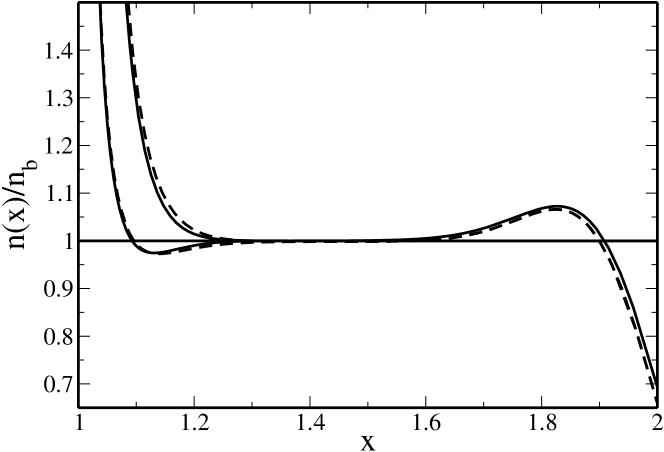
Figure 3: The normalized one-body density $n^{\text{gh}}(x)/n_{b}$, in the grounded horizon case. The dashed lines correspond to a numerical evaluation, obtained from (199), with $N=100$, $x_{m}=2$ and $\alpha=4.15493$ and truncating the sum to 301 terms (the lower value of $k$ is $-200$). The gap close to the metallic boundary has been chosen equal to $w=0.01$. The full lines correspond to the asymptotic result in the fixed shape limit when $\alpha\to\infty$, and $x_{m}=2$ fixed. The two upper curves correspond to a fugacity given by $\zeta\sqrt{\alpha}/(2n_{b})=\tilde{\zeta}L\sqrt{\pi/n_{b}}=1$, while the two lower ones correspond to $\tilde{\zeta}L\sqrt{\pi/n_{b}}=0.1$. Notice how the value of the fugacity only affects the density profile close to the metallic boundary $x=1$.

Interestingly, one again, the density profile shows a universality feature, in the sense that it is essentially the same as for a flat space. As in the flat space, the fugacity controls the excess charge which accumulates near the metallic wall. Only the density profile close to the metallic wall depends on the fugacity. In the bulk, the density is constant, equal to the background density. Close to the other boundary (the hard wall one), the density profile is the same as in the other models from previous sections, and it does not depend on the fugacity.

V Conclusions

The two-dimensional one-component classical plasma has been studied on Flamm’s paraboloid (the Riemannian surface obtained from the spatial part of the Schwarzchild metric). The one-component classical plasma had long been used as the simplest microscopic model to describe many Coulomb fluids such as electrolytes, plasmas, molten salts N. H. March, and M. P. Tosi (1984). Recently it has also been studied on curved surfaces as the cylinder, the sphere, and the pseudosphere. From this point of view, this work presents new results as it describes the properties of the plasma on a surface that had never been considered before in this context.

The Coulomb potential on this surface has been carefully determined. When we limit ourselves to study only the upper or lower half parts ($\mathcal{S}_{\pm}$) of the surface (see Fig. 1) the Coulomb potential is $G^{\text{hs}}({\bf q},{\bf q}^{\prime})=-\ln|z-z^{\prime}|+\text{constant}$, with the appropriate set of coordinates $(x,\varphi)$ defined in section II.0.2, and $z=xe^{i\varphi}$. When charges from the upper part are allowed to interact with particles from the lower part then the Coulomb potential turns out to be $G^{\text{ws}}({\bf q},{\bf q}^{\prime})=-\ln(|z-z^{\prime}|/\sqrt{|zz^{\prime}|})+\text{constant}$. When the charges live in the upper part with the horizon grounded, the Coulomb potential can be determined using the method of images form electrostatics.

Since the Coulomb potential takes a form similar to the one of a flat space, this allows to use the usual techniques Jancovici (1981); A. Alastuey and B. Jancovici (1981) to compute the thermodynamic properties when the coupling constant $\Gamma=\beta q^{2}=2$.

Two different thermodynamic limits have been considered: the one where the radius $R$ of the “disk” confining the plasma is allowed to become very big while keeping the surface hole radius $M$ constant, and the one where both $R\to\infty$ and $M\to\infty$ with the ratio $R/M$ kept constant (fixed shape limit). In both limits we computed the free energy up to corrections of order $O(1)$.

The plasma on half surface is found to be thermodynamically stable, in both types of thermodynamic limit, upon choosing the arbitrary additive constant in the Coulomb potential equal to $-\ln M+\text{constant}$. The system on the full surface is found to be stable upon choosing the constant in the Coulomb potential equal to $-\ln(Mx_{m})+\text{constant}$ where $x_{m}=(\sqrt{R}+\sqrt{R-2M})^{2}/(2M)$.

In the limit $R\to\infty$ while keeping $M$ fixed, most of the surface available to the particles is almost flat, therefore the bulk free energy is the same as in flat space, but corrections from the flat case, due to the curvature effects, appear in the terms proportional to $R$ and the terms proportional to $\ln R$. These corrections are different for each case (half or whole surface).

The asymptotic expansion at fixed shape ($\alpha\to\infty$) presents a different value for the bulk free energy than in the flat space, due to the curvature corrections. On the other hand, the perimeter corrections to the free energy turn out to be the same as for a flat space. This expansion of the free energy does not exhibit the logarithmic correction, $\ln\alpha$, in agreement with the fact that the Euler characteristic of this surface vanishes.

For completeness, we also studied the system on half surface letting the particles interact through the Coulomb potential $G^{\text{ws}}$. In this mixed case the result for the free energy is simply one-half the one found for the system on the full surface.

In the case where the “horizon” is grounded (metallic boundary), the system is studied in the grand canonical ensemble. The limit $R\to\infty$ with $M$ fixed, reproduces the same results as the case of the half surface with potential $G^{\text{hs}}$ up to $O(1)$ corrections, because the effects of the size of the metallic boundary remain $O(1)$. More interesting is the thermodynamic limit at fixed shape, where we find that the bulk thermodynamics are the same as for the half surface with potential $G^{\text{hs}}$, but a perimeter correction associated to the metallic boundary appears. This turns out to be the same as for a flat space. This perimeter correction (“surface” tension) $\beta\gamma_{\text{metal}}$ depends on the value of the fugacity. In the grand canonical formalism, the system can be nonneutral, in the bulk the system is locally neutral, and the excess charge is found near the metallic boundary. In contrast, the outer hard wall boundary (at $x=x_{m}$), exhibits the same density profile as in the other cases, independent of the value of the fugacity. This reflects in a perimeter contribution $\beta\gamma_{\text{hard}}$ equal to the one of the previous cases.

The plasma on Flamm’ s paraboloid is not homogeneous due to the fact that the curvature of the surface is not constant. When the horizon shrinks to a point the upper half surface reduces to a plane and one recovers the well known result valid for the one component plasma on the plane. In the same limit the whole surface reduces to two flat planes connected by a hole at the origin.

We carefully studied the one body density for several different situations: plasma on half surface with potential $G^{\text{hs}}$ and $G^{\text{ws}}$, plasma on the whole surface with potential $G^{\text{ws}}$, and plasma on half surface with the horizon grounded. When only one-half of the surface is occupied by the plasma, if we use $G^{\text{hs}}$ as the Coulomb potential, the density shows a peak in the neighborhoods of each boundary, tends to a finite value at the boundary and to the background density far from it, in the bulk. If we use $G^{\text{ws}}$, instead, the qualitative behavior of the density remains the same. In the thermodynamic limit at fixed shape, we find that the density profile is the same as in flat space near a hard wall, regardless of the Coulomb potential used.

In the grounded horizon case the density reaches the background density far from the boundaries. In this case, the fugacity and the background density control the density profile close to the metallic boundary (horizon). In the bulk and close to the outer hard wall boundary, the density profile is independent of the fugacity. In the thermodynamic limit at fixed shape, the density profile is the same as for a flat space.

Internal and external screening sum rules have been briefly discussed. Nevertheless, we think that systems with non constant curvature should deserve a revisiting of all the common sum rules for charged fluids.

Appendix A Green function of Laplace equation

In this appendix, we illustrate the calculation of the Green function using the original system of coordinates $(r,\varphi)$. The Coulomb potential generated at ${\bf q}=(r,\varphi)$ by a unit charge placed at ${\bf q}_{0}=(r_{0},\varphi_{0})$ with $r_{0}>2M$ satisfies the Poisson equation

$$\Delta G(r,\varphi;r_{0},\varphi_{0})=-2\pi\delta(r-r_{0})\delta(\varphi-\varphi_{0})/\sqrt{g}~{},$$ (205)

where $g=\det(g_{\mu\nu})=r^{2}/(1-2M/r)$. To solve this equation, we expand the Green function $G$ and the second delta distribution in a Fourier series as follows

$$G(r,\varphi;r_{0},\varphi_{0}) = \sum_{n=-\infty}^{\infty}e^{in(\varphi-\varphi_{0})}g_{n}(r,r_{0})~{},$$ (206)

$$\delta(\varphi-\varphi_{0}) = \frac{1}{2\pi}\sum_{n=-\infty}^{\infty}e^{in(\varphi-\varphi_{0})}~{},$$ (207)

to obtain an ordinary differential equation for $g_{n}$

$$\left[\left(1-\frac{2M}{r}\right)\frac{\partial^{2}}{\partial r^{2}}+\left(\frac{1}{r}-\frac{M}{r^{2}}\right)\frac{\partial}{\partial r}-\frac{n^{2}}{r^{2}}\right]g_{n}(r,r_{0})=-\delta(r-r_{0})/\sqrt{g}~{}.$$ (208)

To solve this equation we first solve the homogeneous one for $r<r_{0}$: $g_{n,-}(r,r_{0})$ and $r>r_{0}$: $g_{n,+}(r,r_{0})$. The solution is, for $n\neq 0$,

$$g_{n,\pm}(r,r_{0})=A_{n,\pm}(\sqrt{r}+\sqrt{r-2M})^{2n}+B_{n,\pm}(\sqrt{r}+\sqrt{r-2M})^{-2n}~{},$$ (209)

and, for $n=0$, one finds

$$g_{0,\pm}(r,r_{0})=A_{0,\pm}+B_{0,\pm}\ln(\sqrt{r}+\sqrt{r-2M})~{}.$$ (210)

The form of the solution immediately suggest that it is more convenient to work with the variable $x=(\sqrt{r}+\sqrt{r-2M})^{2}/(2M)$. For this reason, we introduced this new system of coordinates $(x,\varphi)$ which is used in the main text.

Appendix B Asymptotic expansions of $\mathcal{B}_{N}(k)$, $\tilde{\mathcal{B}}_{N}(k)$ and $\hat{\mathcal{B}}_{N}(k)$

B.1 Asymptotic expansion of $\mathcal{B}_{N}(k)$

B.1.1 Limit $N\to\infty$, $x_{m}\to\infty$, and fixed $\alpha$

Doing the change of variable $s=\alpha p(x)$ in the integral (55), we have

$$\mathcal{B}_{N}(k)=\frac{1}{n_{b}}\int_{0}^{N}x^{2k}e^{-\alpha h(x)}\,ds$$ (211)

where $x$ is related to the variable of integration $s$ by $s=\alpha p(x)$. The limit $k\to\infty$ and $N\to\infty$ can be obtained using Laplace method C. M. Bender, and S.  A.  Orzag (1999). To this end, let us write $\mathcal{B}_{N}(k)$ as

$$\mathcal{B}_{N}(k)=\frac{k}{n}\int_{0}^{N/k}e^{k\phi_{k}(t)}\,dt$$ (212)

where we made the change of variable $t=s/k$ and we defined

$$\phi_{k}(t)=2\ln x-\frac{\alpha}{k}\,h(x)$$ (213)

where

$$x=p^{-1}(kt/\alpha)\,.$$ (214)

The derivative of $\phi_{k}$ is

$$\phi_{k}^{\prime}(t) = \frac{1}{x}\frac{dx}{dt}(1-t)$$ (215)

$$= \frac{2k}{\alpha xp^{\prime}(x)}(1-t)$$ (216)

where we have used the definition (214) of $x$ and the properties (41) of $h$ and $p$.

The maximum of $\phi_{k}(t)$ is obtained when $t=1$. At this point we have

$$\phi_{k}^{\prime\prime}(1) = -\frac{2k}{\alpha\hat{x}_{k}p^{\prime}(\hat{x}_{k})}=-1+O(1/\sqrt{k})$$ (217a)

$$\phi_{k}^{(3)}(1) = \frac{4k^{2}}{\alpha^{2}}\frac{p^{\prime}(\hat{x}_{k})+x_{k}p^{\prime\prime}(\hat{x}_{k})}{\hat{x}_{k}^{2}p^{\prime}(\hat{x}_{k})^{3}}=2+O(1/\sqrt{k})$$ (217b)

$$\phi_{k}^{(4)}(1) = \frac{6k^{3}}{\alpha^{3}p^{\prime}(\hat{x}_{k})}\frac{d}{dx}\left[\frac{p^{\prime}(x)+xp^{\prime\prime}(x)}{x^{2}p^{\prime}(x)^{3}}\right]_{x=\hat{x}_{k}}=-6+O(1/\sqrt{k})$$ (217c)

where

$$\hat{x}_{k}=p^{-1}(k/\alpha)\,.$$ (218)

Expanding $\phi_{k}(t)$ up to order $(t-1)^{4}$, and defining $v=\sqrt{k|\phi^{\prime\prime}_{k}(1)|}\,(t-1)$, we have

$$\mathcal{B}_{N}(k) = \frac{\sqrt{k}e^{k\phi_{k}(1)}}{n\sqrt{|\phi^{\prime\prime}_{k}(1)|}}\,\int_{-\sqrt{k|\phi^{\prime\prime}_{k}(1)|}}^{(N-k)\sqrt{|\phi^{\prime\prime}_{k}(1)|/k}}e^{-v^{2}/2}$$ (219)

$$\times\left[1+\frac{v^{3}\phi^{(3)}_{k}(1)}{3!\sqrt{k}|\phi^{\prime\prime}_{k}(1)|^{3/2}}+\frac{v^{4}\phi_{k}^{(4)}(1)}{4!k|\phi^{\prime\prime}_{k}(1)|^{2}}+\frac{v^{6}[\phi^{(3)}_{k}(1)]^{2}}{3!^{2}2k|\phi^{\prime\prime}_{k}(1)|^{3}}+o\left(\frac{1}{k}\right)\right]\,dv\,.$$

Let us define

$$\epsilon_{k}=\sqrt{|\phi^{\prime\prime}_{k}(1)|}\,\frac{N-k}{\sqrt{2k}}=\frac{N-k}{\sqrt{2N}}+O(1/\sqrt{N})$$ (220)

which is an order one parameter, since we are interested in an expansion for $N$ and $k$ large with $N-k$ of order $\sqrt{N}$. Using the integrals

$$\int_{-\infty}^{\epsilon}e^{-v^{2}/2}\,dv = \sqrt{\frac{\pi}{2}}\left[1+\mathop{\text{missing}}{erf}\left(\frac{\epsilon}{\sqrt{2}}\right)\right]$$ (221)

$$\int_{-\infty}^{\epsilon}e^{-v^{2}/2}\,v^{3}\,dv = -(2+\epsilon^{2})e^{-\epsilon^{2}/2}$$ (222)

$$\int_{-\infty}^{\epsilon}e^{-v^{2}/2}\,v^{4}\,dv = 3\sqrt{\frac{\pi}{2}}\left[1+\mathop{\text{missing}}{erf}\left(\frac{\epsilon}{\sqrt{2}}\right)\right]-e^{-\epsilon^{2}/2}\epsilon(3+\epsilon^{2})$$ (223)

$$\int_{-\infty}^{\epsilon}e^{-v^{2}/2}\,v^{6}\,dv = 15\sqrt{\frac{\pi}{2}}\left[1+\mathop{\text{missing}}{erf}\left(\frac{\epsilon}{\sqrt{2}}\right)\right]-e^{-\epsilon^{2}/2}\epsilon(15+5\epsilon^{2}+\epsilon^{4})$$ (224)

where $\mathop{\text{missing}}{erf}(z)=(2/\sqrt{\pi})\int_{0}^{z}e^{-u^{2}}\,du$ is the error function, we find in the limit $N\to\infty$, $k\to\infty$, and finite $\epsilon_{k}$,

$$\mathcal{B}_{N}(k) = \sqrt{\frac{\pi k}{2|\phi^{\prime\prime}_{k}(1)|}}\frac{e^{k\phi_{k}(1)}}{n}\left[1+\mathop{\text{missing}}{erf}\left({\epsilon_{k}}\right)\right]\left[1+\frac{1}{12k}+\frac{1}{\sqrt{k}}\,\xi_{1}(\epsilon_{k})+\frac{1}{k}\,\xi_{2}(\epsilon_{k})\right]\,.$$ (225)

The functions $\xi_{1}(\epsilon_{k})$ and $\xi_{2}(\epsilon_{k})$ contain terms proportional $e^{-\epsilon_{k}^{2}}$, from the Gaussian integrals above. However, as explained in the main text, these do not contribute to the final result for the partition function up to order $O(1)$, because the exponential term $e^{-\epsilon_{k}^{2}}$ make convergent and finite the integrals of these functions that appear in the calculations, giving terms of order $O(1)$ and $O(1/\sqrt{N})$ respectively.

B.1.2 Limit $N\to\infty$, $\alpha\to\infty$, fixed $x_{m}$

For the determination of the thermodynamic limit at fixed shape, we also need the asymptotic behavior of $\mathcal{B}_{N}(k)$ when $\alpha\to\infty$ at fixed $x_{m}$. We write $\mathcal{B}_{N}(k)$ as

$$\mathcal{B}_{N}(k)=\frac{\alpha}{n_{b}}\int_{1}^{x_{m}}e^{-\alpha[h(x)-2p(\hat{x}_{k})\ln x]}\,p^{\prime}(x)\,dx\,,$$ (226)

where we have defined once again $\hat{x}_{k}$ by $k=\alpha p(\hat{x}_{k})$. We apply Laplace method for $\alpha\to\infty$. Let

$$F(x)=h(x)-2p(\hat{x}_{k})\ln x\,.$$ (227)

$F$ has a minimum for $x=\hat{x}_{k}$ with $F^{\prime\prime}(\hat{x}_{k})=2p^{\prime}(\hat{x}_{k})/\hat{x}_{k}$. Expanding to the order $(x-\hat{x}_{k})^{2}$ the argument of the exponential and following calculations similar to the ones of the previous section, we find

$$\mathcal{B}_{N}(k) = \frac{\sqrt{\alpha\pi\hat{x}_{k}p^{\prime}(\hat{x}_{k})}}{2n_{b}}e^{-\alpha[h(\hat{x}_{k})-2p(\hat{x}_{k})\ln\hat{x}_{k}]}\left[\mathop{\text{missing}}{erf}(\epsilon_{k,1})+\mathop{\text{missing}}{erf}(\epsilon_{k,m})\right]$$ (228)

$$\times\left(1+\frac{1}{\alpha}\xi_{0}(\hat{x}_{k})+\frac{1}{\sqrt{\alpha}}\left[\xi_{1,m}(\epsilon_{k,m})+\xi_{1,1}(\epsilon_{k,1})\right]\right)$$

where

$$\epsilon_{k,m} = \sqrt{\frac{\alpha p^{\prime}(x_{m})}{x_{m}}}(x_{m}-\hat{x}_{k})\,,$$ (229)

$$\epsilon_{k,1} = \sqrt{\alpha p^{\prime}(1)}(\hat{x}_{k}-1)\,.$$ (230)

The terms with the error functions come from incomplete Gaussian integral and take into account the contribution of values of $k$ such that $x_{m}-\hat{x}_{k}$ (or $\hat{x}_{k}-1$) is of order $1/\sqrt{\alpha}$, or equivalently $N-k$ (or $k$) of order $\sqrt{N}$.

The functions $\xi_{0}(\hat{x}_{k})$, $\xi_{1,1}(\epsilon_{k,1})$, and $\xi_{1,m}(\epsilon_{k,m})$ can be computed explicitly, pushing the expansion one order further. These next order corrections are different than in the previous section, in particular $(1/\alpha)\xi_{0}(\hat{x}_{k})\neq 1/(12k)$.

However, these next order terms are not needed in the computation of the partition function at order $O(1)$, since they give contributions of order $O(1)$. Note in particular that the term $\xi_{0}(\hat{x}_{k})/\alpha$ gives contributions of order $O(1)$, contrary to the previous limit studied earlier where it gave contributions of order $\ln N$. Indeed, in the logarithm of the partition function, this term gives a contribution

$$\sum_{k=0}^{N}\frac{\xi_{0}(\hat{x}_{k})}{\alpha}=\frac{1}{\alpha}\int_{1}^{x_{m}}\alpha p^{\prime}(x)\xi_{0}(x)\,dx+o(1)=O(1)\,.$$ (231)

B.2 Asymptotic expansions of $\tilde{\mathcal{B}}_{N}(k)$ and $\hat{\mathcal{B}}_{N}(k)$

To study $\tilde{\mathcal{B}}_{N}(k)$, it is convenient to define $k^{\prime}=k-\frac{N}{2}$, then

$$\tilde{\mathcal{B}}_{N}(k)=\frac{\alpha}{n_{b}}\int_{1/x_{m}}^{x_{m}}x^{2k^{\prime}}e^{-\alpha h(x)}\,x\,p^{\prime}(x)\,dx\,,$$ (232)

which is very similar to

$$\hat{\mathcal{B}}_{N}(k)=\frac{\alpha}{n_{b}}\int_{1}^{x_{m}}x^{2k}e^{-\alpha h(x)}\,x\,p^{\prime}(x)\,dx\,.$$ (233)

changing $k^{\prime}$ by $k$, and taking into account the extended domain of integration $[1/x_{m},1]$ for $\tilde{\mathcal{B}}_{N}$. As in the previous section, the asymptotic expansions for $\tilde{\mathcal{B}}_{N}(k)$ and $\hat{\mathcal{B}}_{N}(k)$ can be obtained using Laplace method. Notice that for $\tilde{\mathcal{B}}_{N}(k)$, $k^{\prime}$ is in the range $[-\frac{N}{2},\frac{N}{2}]$. When $k^{\prime}<0$, the maximum of the integrand is in the region $[1/x_{m},1]$, and when $k^{\prime}>0$, the maximum is in the region $[1,x_{m}]$. Due to the fact that the contribution to the integral from the region $[1/x_{m},1]$ is negligible when $k^{\prime}>0$, the asymptotics for $\hat{\mathcal{B}}_{N}(k)$ will be the same as those for $\tilde{\mathcal{B}}_{N}(k)$, for $k^{\prime}>0$, doing the change $k\to k^{\prime}$. Therefore, we present only the derivation of the asymptotics of $\tilde{\mathcal{B}}_{N}$.

B.2.1 Limit $N\to\infty$, $x_{m}\to\infty$, and fixed $\alpha$

We proceed as for ${\mathcal{B}}_{N}(k)$, defining the variable of integration $t=\alpha p(x)/k^{\prime}$, then

$$\tilde{\mathcal{B}}_{N}(k)=\frac{|k^{\prime}|}{n_{b}}\int_{-\frac{N}{2|k^{\prime}|}}^{\frac{N}{2|k^{\prime}|}}x\,e^{k^{\prime}\phi_{k^{\prime}}(t)}\,dt$$ (234)

where $\phi_{k^{\prime}}(t)$ is the same function defined in equation (213). Now we apply Laplace method to compute this integral. The main difference with the calculations done for $\mathcal{B}_{N}$ are the following. First, taking into account that $k^{\prime}$ can be positive or negative, we should note that

$$\phi_{k^{\prime}}^{\prime\prime}(1) = \begin{cases}-1+O(1/\sqrt{|k^{\prime}|})&k^{\prime}>0\\ 1+O(1/\sqrt{|k^{\prime}|})&k^{\prime}<0\end{cases}$$ (235)

$$\phi_{k^{\prime}}^{(3)}(1) = \begin{cases}2+O(1/\sqrt{|k^{\prime}|})&k^{\prime}>0\\ -2+O(1/\sqrt{|k^{\prime}|})&k^{\prime}<0\end{cases}$$ (236)

$$\phi_{k^{\prime}}^{(4)}(1) = \begin{cases}-6+O(1/\sqrt{|k^{\prime}|})&k^{\prime}>0\\ 6+O(1/\sqrt{|k^{\prime}|})&k^{\prime}<0\end{cases}$$ (237)

Second, we also need to expand $x$ close to the maximum which is obtained for $t=1$,

$$x=\hat{x}_{k^{\prime}}[1+a(t-1)+b(t-1)^{2}+O((t-1)^{3})]$$ (238)

with

$$a=\frac{p(\hat{x}_{k^{\prime}})}{\hat{x}_{k^{\prime}}p^{\prime}(\hat{x}_{k^{\prime}})}=\begin{cases}\frac{1}{2}+O(1/\sqrt{|k^{\prime}|})&k^{\prime}>0\\ -\frac{1}{2}+O(1/\sqrt{|k^{\prime}|})&k^{\prime}<0\end{cases}$$ (239)

and

$$b=-\frac{p(\hat{x}_{k^{\prime}})^{2}p^{\prime\prime}(\hat{x}_{k^{\prime}})}{2\hat{x}_{k^{\prime}}p^{\prime}(\hat{x}_{k^{\prime}})^{3}}=\begin{cases}-\frac{1}{8}+O(1/\sqrt{|k^{\prime}|})&k^{\prime}>0\\ \frac{3}{8}+O(1/\sqrt{|k^{\prime}|})&k^{\prime}<0\end{cases}$$ (240)

Notice in particular that for the term $b$, the difference between positive and negative values of $k^{\prime}$ is not only a change of sign. This is to be expected since the function $x$ is not invariant under the change $x\to 1/x$.

Following very similar calculations to the ones done for $\mathcal{B}_{N}$ with the appropriate changes mentioned above, we finally find

$$\tilde{B}_{N}(k) = \frac{\hat{x}_{k^{\prime}}}{2n_{b}}\sqrt{\pi\alpha\hat{x}_{k^{\prime}}p^{\prime}(\hat{x}_{k^{\prime}})}e^{-\alpha[h(\hat{x}_{k^{\prime}})-2p(\hat{x}_{k^{\prime}})\ln\hat{x}_{k^{\prime}}]}$$ (241)

$$\times\left[\mathop{\text{missing}}{erf}\left(\epsilon_{k,\min}\right)+\mathop{\text{missing}}{erf}\left(\epsilon_{k,\max}\right)\right]\left[1+\left(\frac{1}{12}+c\right)\frac{1}{|k^{\prime}|}+\cdots\right]$$

with

$$c=\begin{cases}\frac{3}{8}&k^{\prime}>0\\ -\frac{1}{8}&k^{\prime}<0\end{cases}$$ (242)

and

$$\epsilon_{k,\max} = \sqrt{\frac{\alpha p^{\prime}(x_{m})}{x_{m}}}(x_{m}-\hat{x}_{k-\frac{N}{2}})\,,$$ (243a)

$$\epsilon_{k,\min} = \sqrt{\frac{\alpha p^{\prime}(1/x_{m})}{1/x_{m}}}\left(\hat{x}_{k-\frac{N}{2}}-\frac{1}{x_{m}}\right)\,.$$ (243b)

The dots in (241) represent contributions of lower order and of functions of $\epsilon_{k,\min}$ and $\epsilon_{k,\max}$ that give $O(1)$ contributions to the partition function. Comparing to the asymptotics of $\mathcal{B}_{N}$ we notice two differences: the factor $\hat{x}_{k^{\prime}}$ multiplying all the expressions and the correction $c/|k^{\prime}|$.

B.2.2 Limit $N\to\infty$, $\alpha\to\infty$, and fixed $x_{m}$

The asymptotic expansion of $\tilde{\mathcal{B}}_{N}$ in this fixed shape situation is simpler, since we do not need the terms of order $1/\alpha$. Doing similar calculations as the ones done for $\mathcal{B}_{N}$ taking into account the additional factor $x$ in the integral we find

$$\tilde{\mathcal{B}}_{N}(k) = \frac{\hat{x}_{k^{\prime}}\sqrt{\alpha\pi\hat{x}_{k^{\prime}}p^{\prime}(\hat{x}_{k^{\prime}})}}{2n_{b}}e^{-\alpha[h(\hat{x}_{k^{\prime}})-2p(\hat{x}_{k^{\prime}})\ln\hat{x}_{k^{\prime}}]}\left[\mathop{\text{missing}}{erf}(\epsilon_{k,\min})+\mathop{\text{missing}}{erf}(\epsilon_{k,\max})\right]\,.$$ (244)

References

• S. F. Edwards and A. Lenard (1962) S. F. Edwards and A. Lenard, J. Math. Phys. 3, 778 (1962).
• Jancovici (1981) B. Jancovici, Phys. Rev. Lett. 46, 386 (1981).
• A. Alastuey and B. Jancovici (1981) A. Alastuey and B. Jancovici, J. Phys. (France) 42, 1 (1981).
• B. Jancovici and G. Téllez (1996) B. Jancovici and G. Téllez, J. Stat. Phys. 82, 609 (1996).
• B. Jancovici, G. Manificat, and C. Pisani (1994) B. Jancovici, G. Manificat, and C. Pisani, J. Stat. Phys. 76, 307 (1994).
• M. L. Rosinberg, L. Blum (1984) M. L. Rosinberg, L. Blum, J. Chem. Phys. 81, 3700 (1984).
• Ph. Choquard (1981) Ph. Choquard, Helv. Phys. Acta 54, 332 (1981).
• Ph. Choquard, P. J. Forrester, and E. R. Smith (1983) Ph. Choquard, P. J. Forrester, and E. R. Smith, J. Stat. Phys. 33, 13 (1983).
• Caillol (1981) J. M. Caillol, J. Phys. (Paris) – Lett. 42, L (1981).
• P. J. Forrester, B. Jancovici, and J. Madore (1992) P. J. Forrester, B. Jancovici, and J. Madore, J. Stat. Phys. 69, 179 (1992).
• P. J. Forrester and B. Jancovici (1996) P. J. Forrester and B. Jancovici, J. Stat. Phys. 84, 337 (1996).
• G. Téllez and P. J. Forrester (1999) G. Téllez and P. J. Forrester, J. Stat. Phys. 97, 489 (1999).
• Jancovici (2000) B. Jancovici, J. Stat. Phys. 99, 1281 (2000).
• B. Jancovici and G. Téllez (1998) B. Jancovici and G. Téllez, J. Stat. Phys. 91, 953 (1998).
• R. Fantoni, B. Jancovici, and G. Téllez (2003) R. Fantoni, B. Jancovici, and G. Téllez, J. Stat. Phys. 112, 27 (2003).
• B. Jancovici and G. Téllez (2004) B. Jancovici and G. Téllez, J. Stat. Phys. 116, 205 (2004).
• Kaniadakis (2002) G. Kaniadakis, Phys. Rev. E 66, 056125 (2002).
• Kaniadakis (2005) G. Kaniadakis, Phys. Rev. E 72, 036108 (2005).
• Ginibre (1965) J. Ginibre, J. Math. Phys. 6, 440 (1965).
• M. L. Mehta (1991) M. L. Mehta, Random Matrices (Academic Press, 1991).
• M. Abramowitz and A. Stegun (1965) M. Abramowitz and A. Stegun, ”Handbook of mathematical functions” (Dover, New York, 1965).
• R. Wong (1989) R. Wong, Asymptotic Approximations of Integrals (Academic Press, 1989).
• B. Jancovici (1982) B. Jancovici, J. Stat. Phys. 28, 43 (1982).
• Ph. A. Martin (1988) Ph. A. Martin, Rev. Mod. Phys. 60, 1075 (1988).
• P. J. Forrester (1985) P. J. Forrester, J. Phys. A: Math. Gen. 18, 1419 (1985).
• Zinn-Justin (1993) J. Zinn-Justin, ”Quantum Field Theory and Critical Phenomena” (Clarendon Press, Oxford, 1993), 2nd ed.
• N. H. March, and M. P. Tosi (1984) N. H. March, and M. P. Tosi, ”Coulomb liquids” (Academic Press, 1984).
• C. M. Bender, and S.  A.  Orzag (1999) C. M. Bender, and S.  A.  Orzag, Advanced Mathematical Methods for Scientists and Engineers: Asymptotic Methods and Perturbation Theory (Springer, 1999).