A cellular automata model for avascular solid tumor growth under the effect of therapy
Abstract
Tumor growth has long been a target of investigation within the context of mathematical and computer modelling. The objective of this study is to propose and analyze a two-dimensional probabilistic cellular automata model to describe avascular solid tumor growth, taking into account both the competition between cancer cells and normal cells for nutrients and/or space and a time-dependent proliferation of cancer cells. Gompertzian growth, characteristic of some tumors, is described and some of the features of the time-spatial pattern of solid tumors, such as compact morphology with irregular borders, are captured. The parameter space is studied in order to analyze the occurrence of necrosis and the response to therapy. Our findings suggest that transitions exist between necrotic and non-necrotic phases (no-therapy cases), and between the states of cure and non-cure (therapy cases). To analyze cure, the control and order parameters are, respectively, the highest probability of cancer cell proliferation and the probability of the therapeutic effect on cancer cells. With respect to patterns, it is possible to observe the inner necrotic core and the effect of the therapy destroying the tumor from its outer borders inwards.
keywords:
tumor growth, cellular automata, parameter space, necrosis, therapy1 INTRODUCTION
Neoplastic diseases are the cause of 7 million deaths annually or 12of deaths worldwide [1]. Mathematical and computer modelling may lead to greater understanding of the dynamics of cancer progression in the patient [2] [3]. These techniques may also be useful in selecting better therapeutic strategies by subjecting available options to computer testing (in silico). Continuous models have been proposed to describe the stages of tumor growth since the middle of the 20th century [4]. Initially, a tumor grows exponentially (linear rate). After this transient stage, the growth rate decreases and a steady state is attained, due to several factors including a lack of nutrients and hypoxia. This nonlinear behavior characterizes avascular tumor growth when neovascularization has not yet been triggered. The decelerating avascular growth may be guided by different rules such as, for example, Gompertzian and logistic functions. Gompertzian growth has been one of the most studied decelerating tumor growth over the past 60 years [5], [6] [7]. It is found, for example, in some solid tumors such as breast carcinomas [8] [9]. It is also observed in tumors in vitro [10] [11].
Although continuous models are capable of describing the behavior of tumor growth, it would appear more reasonable to adopt a discrete approach when describing the prevascular stage. Due to the fact that the angiogenic process has not triggered early tumor growth, few cancer cells are present and growth depends predominantly on the interactions of these cells with adjacent cells and with the environment [12]. In addition, in the discrete approach, it is easier to capture the time-spatial pattern generated by the model in order to compare it with actual patterns [13]. Some cellular automata models [14] [15] and hybrid cellular automata [12] [16] [17] have been proposed to study tumor growth.
Another important topic that is analyzed in mathematical models is the response to therapy, including how tumor growth changes under the effect of a drug [18]. The focus is directed towards identifying the optimal therapy to maximize the effect on cancer cells and minimize the effect on normal cells [19] [20]. Although various continuous chemotherapy models exist [21], [22], [23], to the best of our knowledge the majority of the discrete models cited in the literature have not yet been used to investigate this topic.
The objective of this work is to propose a two-dimensional cellular automata model consisting of 4 states (empty site, normal cell, cancer cell or necrotic tumor cell) to describe avascular tumor growth. It should be emphasized that in this study the term tumor growth is used to refer to the number of cancer cells rather than the volume of the tumor; in other words, it is assumed that the tumor volume is proportional to the number of cancer cells [4]. Assuming that the angiogenic process has not yet been triggered, there is no increase in nutrients, which are uniformly distributed over the lattice. In this simple model, some relevant processes involved in the prevascular phase of tumor growth are assessed: a dynamic proliferation of cancer cells and the competition between normal cells and cancer cells for nutrients and/or space. Since necrosis is often present in the prevascular stage of tumor growth [10] [24], the possibility of necrosis in the model must also be taken into consideration. Finally, the effect of therapy is included in order to investigate whether the system evolves to a state of cure.
This paper is organized as follows. In section 2, the model is presented, together with its local rules, parameters and the scope of the algorithm. Section 3 describes the simulated time series of cell density in the presence or absence of treatment, and shows the features of the time-spatial pattern of simulated solid tumors. In section 4, the parameter related to the process of necrosis and the effect of therapy is analyzed. Finally, in section 5, our results are discussed from the point of view of the phenomenon and some concluding remarks are made.
2 THE MODEL
We propose a two-dimensional () cellular automata model [25] under periodic boundary conditions, using a Moore neighborhood with a radius of 1. At the initial condition (), there is only one cancer cell (to ensure better visualization, this was taken from the center of the lattice). Since the intention it to model a non-viral tumor, normal cells would not be transformed into cancer cells with the exception of the cancer cell that triggers tumor growth at [26]. The lattice represents a tissue sample; there is a cell in each site that may be in one of four states: normal cell (NoC), cancer cell (CC), necrotic cell (NeC) or empty site (ES). We assume that the nutrients are uniformly available over the lattice. In this respect, lack of space is identified with lack of nutrients in our model.
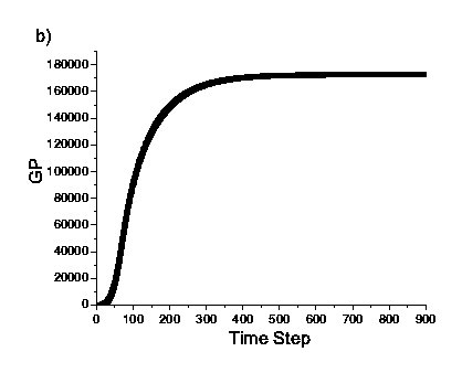
There is a growth potential value associated with each normal or cancer cell. Although the two-dimensional character of the model mimics the in vitro situation, the growth potential of cancer cells simulates the three-dimensional tumor in vivo in the sense that it represents the total number of cancer cells, i.e., in addition to the cancer cells on the lattice, the cancer cells generated by these cells.
The local rules are such that:
-
(i) The initial value of the mitotic probability of cancer cells is represented by a parameter that measures the available resources at the beginning of the tumor. After that, it decreases by a factor until reaching the null value:
(1) in which and are the number of normal and cancer cells at time , respectively. As shown, depends only on the dynamics, setting up a feedback inhibition mechanism [13]: as the tumor grows, decreases because of the combined effect of the decrease in the number of normal cells and the increase in the number of cancer cells. In order to intensify the effect of this mechanism (see [27]), an exponent 2 in equation (1) is considered. Since there is no new available source of nutrients and/or space, it decreases as the density of cancer cells increases because the available nutrients and/or space are reduced. The effect of the proliferation of cancer cells is that their growth potential increases by a unit at each time step.
-
(ii) The cancer cells compete with normal cells for the empty sites, depending on the potential growth of neighboring cells. According to the majority rule, a normal cell is displaced by a cancer cell following local battles occurring between healthy and cancerous cells [15].
-
(iii) If the growth potential of a cancer cell reaches a threshold value that is a fraction of the lattice size , it becomes necrotic and its growth potential falls to zero.
-
(iv) Both normal and cancer cells may die, with probabilities and , respectively, due to the continuous infusion of a drug that is applied after tap time steps; in this case, the site becomes empty.
-
(v) if there are no cancer cells in the neighborhood of a dead cell (empty site), regeneration of normal cells occurs; if the cancer cells in the neighborhood of a necrotic cell die as a result of the therapy, the necrotic cell is eliminated.
The algorithm was computationally implemented in FORTRAN 77 in accordance with the following steps: input data; calculate ; identify the state of the cell (choose one of the subroutines: normal cell (NoC), cancer cell(CC), necrotic cell(NeC), empty site (ES); update the cells of the lattice; after N iterations, output data.
The input data are the following cellular automata (CA) parameters:
-
1) The spatial parameters: lattice size L; necrosis threshold fraction of lattice size;
-
2) The temporal parameters: the length of the time series t final and the initial time of therapy infusion ;
-
3) The probabilities of: the initial proliferation of cancer cells ; the effect of therapy on normal cells and cancer cells ( and ).
The output data are the time series of the density of each type of cell and the final configuration of the lattice at any time step. In addition, the time-spatial configurations, controlled by a package denominated g2 [28] whose commands are inserted into the computer program in FORTRAN, are generated in ”real time”. This package may be used in C, PYTHON and PERL.
The following is a description of each subroutine based on the local rules:
-
a) Normal Cell (NoC) - a random number is compared to . If , the growth potential is confirmed: if , the cell dies and the site becomes empty; otherwise, it remains occupied by a normal cell but . If and if there is at least one neighboring cancer cell, then the normal cell is ’dislocated’, and the site becomes empty; otherwise it remains a normal cell.
-
b) Cancer Cell (CC) - if all of its neighbors are cancer cells and its growth potential reaches a fraction of lattice size , the cancer cell becomes necrotic. Otherwise, a number is randomly chosen. If and , the potential is confirmed: if , it is reduced by a unit and the cell remains a cancer cell; otherwise the cell dies and the site becomes empty. Finally, if , the cell remains a cancer cell; however, its growth potential increases by a unit.
-
c) Necrotic Cell (NeC) - if at least one of its neighbors is neither a cancer cell nor a necrotic cell, it is eliminated and the site becomes empty; otherwise, it continues necrotic.
-
d) Empty Site (ES) - if there are cancer and normal cells in its neighborhood, the local battle between cancer cells and normal cells is such that if the sum of the potential growth of its neighboring cancer cells is greater or equal to the sum of the potential growth of its normal cell neighbors, then the empty site is occupied by a cancer cell that diffuses from one of the randomly chosen neighbors; otherwise, it is occupied by one of the randomly chosen normal cells that were previously dislocated. If there are only normal cells in its neighborhood, it becomes a normal cell through a process of regeneration. Finally, if none of its neighbors are cancer cells or normal cells, it remains empty.
3 RESULTS: SIMULATED TIME SERIES AND TIME-SPATIAL PATTERNS
Computational simulations of the model were performed in order to analyze two classes of behavior: cases in which no treatment was given and treatment cases. In each subsection, the time series of the simulated tumor as well as time-spatial patterns are shown.
3.1 NO TREATMENT CASE
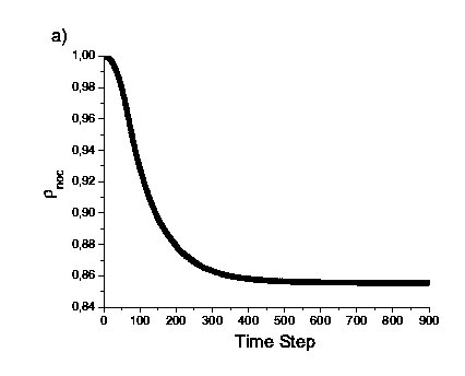
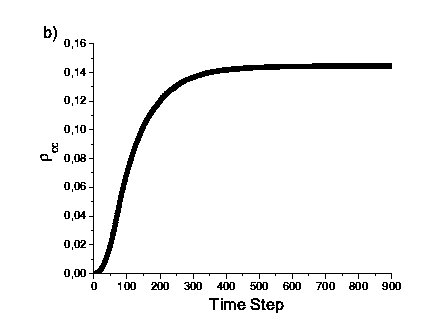
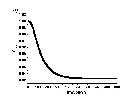
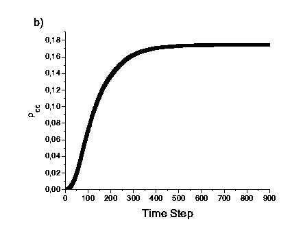
In the case of no treatment, the following parameters are considered: . For fixed values of , and , but different values of , in Figures 1 and 3, the time series of the density of cells for nonnecrotic and necrotic tumors, respectively, are shown. In both cases, the cell densities reach saturated values due to the effects of the competition between normal cells and cancer cells, and the time-dependent mitotic probability. Comparing Figures 1b and 3b, the stationary value of cancer cell density is clearly greater in necrotic tumors than in nonnecrotic ones. This is a consequence of the fact that assumes smaller values in necrotic tumors compared to nonnecrotic ones because it does not depend on the density of necrotic cells. In both cases, the average of the different samples is considered, corresponding to different seeds of random numbers.
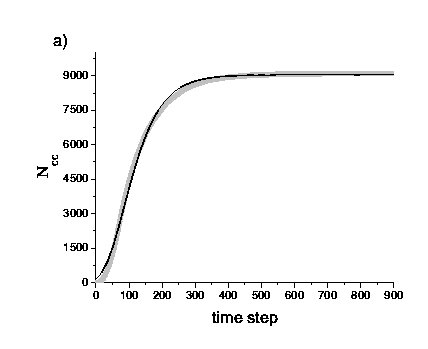
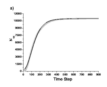
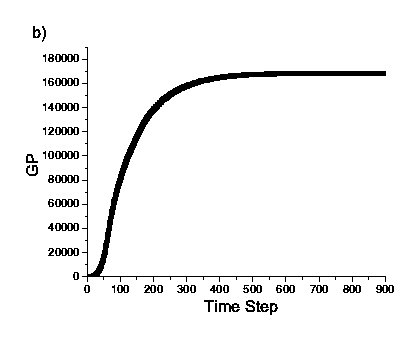
Figures 2a and 4a show that the tumor growth obeys the Gompertzian function both in nonnecrotic and necrotic cases. This behavior is observed with respect to the number of cancer cells for a range of values of . In Gompertzian growth, the specific growth rate of the number of cancer cells decreases logarithmically:
| (2) |
where
-
a) is the initial population of cancer cells;
-
b) is the specific growth rate of cells at ;
-
c) measures how rapidly the curve departs from a singular exponential and curves over, assuming its characteristic shape.
The solution of (2) is
| (3) |
It is evident that the stationary value of is . According to the Gompertzian fitting represented by equation 3, the results of the simulations shown in Figures 2 and 4 correspond respectively to the following parameters:
-
I) The nonnecrotic tumor: , and
-
II) The necrotic tumor: , and
Comparing the above parameters of (I) and (II), the behavior of nonnecrotic and necrotic tumors was found to be very similar. It was also found that the number of cancer cells obeys the Gompertzian fitting.
An important confirmation of our model is shown by comparing the Gompertzian fitting parameters of simulated tumors with the corresponding parameters of actual tumors [6] [7]. For instance, in the case of the testicular tumors shown in Table 3 of reference [6], the values are in the range of . Our simulated values are within the above range if we consider the time step of our simulations to be one day.
In relation to the parameters and , the simulated values are not comparable to the actual values, since no information on the initial size of the tumor was included in our model. Both and are strongly dependent on that information.
Finally, it would be very interesting to discover whether it is possible to relate the cellular automata no-therapy parameters , and with the Gompertzian parameters for the range of values of and to assess whether the number of cancer cells obeys a Gompertzian growth pattern. In this case, some preliminary conclusions may be drawn with respect to : it decreases in accordance with the necrotic parameter but it increases linearly as a function of lattice size and, exponentially with . Concerning the other Gompertzian parameters, the answer to this question is not so simple. Following these conclusions leads us to a much more interesting quandary if we want to make the model more realistic: to estimate realistic ranges of the CA no-therapy parameters , and based on the Gompertzian parameters of actual solid tumors.
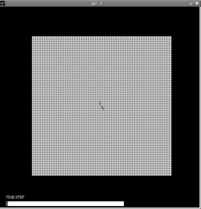
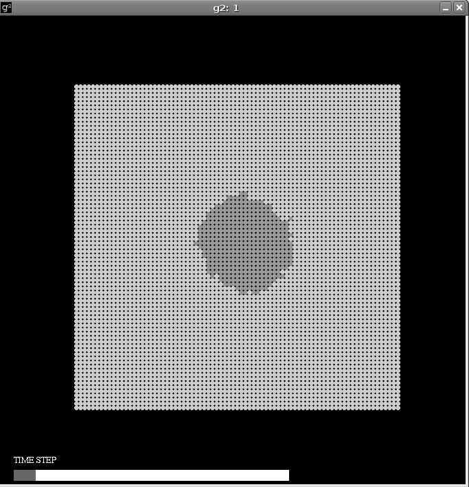
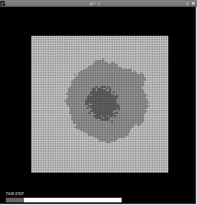
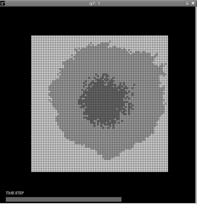
With respect to the time-spatial patterns of the simulated tumors, Figure 5 shows the lattice configuration at some time during the steady state in the necrotic (Figure 5b) cases. Using the g2 package, it was found that, although tumor growth leads to the compact shape that is characteristic of solid tumors, the growth process is such that its boundary is irregular for any time , as, for example, for the time steps represented in Figure 5. A similar type of behavior is observed for the time-spatial patterns in the nonnecrotic tumor. In relation to the process of necrosis, the necrotic region was found to be inside the tumor at any time [29] [10], as shown in Figure 5.
3.2 TREATMENT CASE
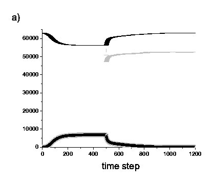
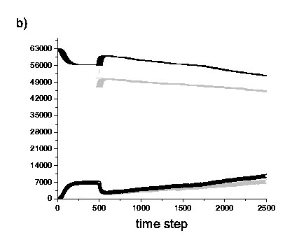
Figures 6a and 6b show the simulated time series of the number of cancer cells and normal cells for the different values of and corresponding to successful treatment (cure) and unsuccessful treatment (non-cure), respectively. In each figure, two values of are considered. It can be clearly seen that, for both values of , the success of the treatment does not change. It is also clear that the tumor size increases until tap (see figures 6a and 6b). However when , the reduction in tumor size starts, as expected, after time steps.
When treatment is successful (), it was found that, for an upper value of (; light grey), more normal cells are eliminated compared with a lower value of - as shown in Figure 6a (dark grey). Therefore, we may conclude that very small values of correspond to optimal therapy. However, in the case of unsuccessful treatment (), when is increased, both a decrease in the number of normal cells and a slower rate of increase of cancer cells is found (see fig 6b).
A systematic analysis of the parameter space presented in the next section will provide a more precise conclusion about the role of parameter.
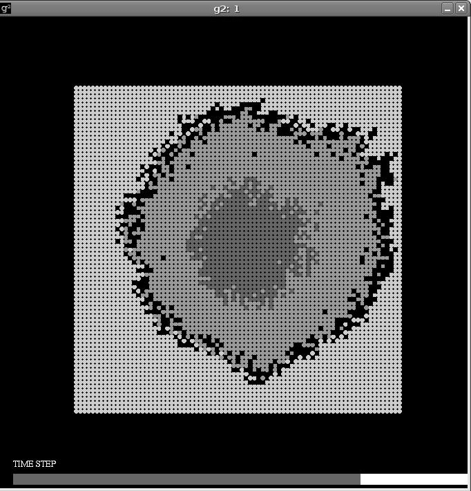
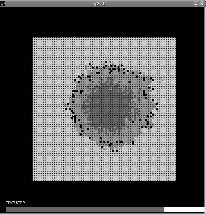
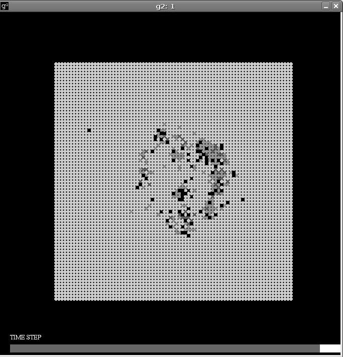
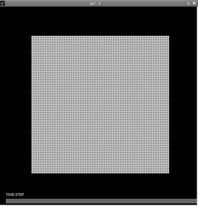
In order to analyze the effect of therapy on cancer cells, the time-spatial distribution of the simulated tumors was followed using the g2 package. Figure 7 shows the configuration of the lattice at different time steps from the beginning of therapy until the tumor is eliminated.
4 RESULTS: PARAMETER SPACE
Analysis of the parameter space is important in order to confirm the robustness of the model and to identify the most relevant parameters for the dynamics of the model.
According to the relevance of some CA parameters to the features of the phenomenon, this analysis of parameter space was divided into two parts: the occurrence of necrosis (no treatment cases) and reaching a state of cure (treatment cases).
4.1 THE OCCURRENCE OF NECROSIS
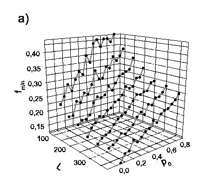
In the first part, the parameters are again established as: with the aim of evaluating the effect of necrosis, and the minimum value of f is obtained for each pair of values . The values of are presumed to range from 101 to 251, increasing the interval by . With respect to , the whole interval from 0.1 to 0.9 is taken into account, increasing . Figure 8 shows that a transition exists between the nonnecrotic (lower) and necrotic (upper) regions of parameter space.
It was found that:
| (4) |
where the linear and the angular coefficients, and are different for distinct values of the lattice size.
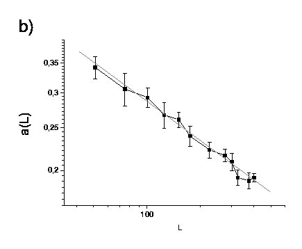
The angular coefficient where and (see figure 8b).
Since the lattice size is an intrinsic parameter of the model, that transition is such that the the maximal growth probability is the control parameter, while the necrotic parameter is the order parameter.
4.2 REACHING THE CURE STATE
If the tumor is submitted to systemic treatment represented by a probability starting at that affects normal cells with a probability , our aim is to establish the minimum value of in order to achieve a state of cure, i.e., no cancer cells.
The analysis is now more complex than the one performed in subsection 4.1 in the sense that there are 4 important parameters that control the behavior of the therapeutic effect: , , , and . The relevance of is evident in subsection 3.2. This analysis is divided into two parts.
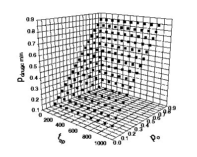
In the first part, motivated by the behavior observed in figure 6a, the parameter is defined as , assuming very small values ( to simulate optimal therapy. Lattice size is also established as and the necrotic parameter . Analogously to the method applied in subsection 4.1, the minimum value of was obtained for each pair of values . The range of values for and tap are, respectively, and . Figure 9 shows the relevant role of dividing the parameter subspace into two regions: the lower is the non-cure state while the upper corresponds to the state of cure. In this case is again the control parameter but is the order parameter.
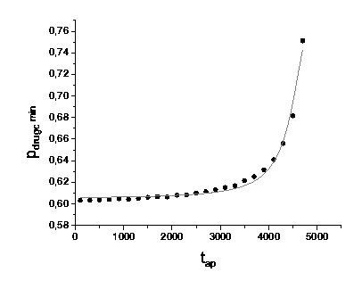
In the second part, a value of remains fixed, while the pair varies , again in order to obtain the minimum value of that would be sufficient to effectively eliminate the tumor, now related to the effect of the drug on the normal cells. The whole interval of was taken into account from very small values until . It would be necessary to extend in order to maintain the duration of application, since in this analysis the parameter varied. Since this behavior is similar for any value of , in figure 10 the minimum value of is shown to increase as a function of in accordance with a Lorentzian function:
This result means that the minimal rate of infusion of the drug to eliminate the tumor has to be greater if the treatment begins later. It emphasizes how important it is to initiate treatment as early as possible in order to reduce the infusion rate of the drug.
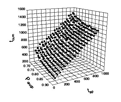
Finally in the cases in which the tumor is eliminated (), for fixed values of , , and , the cure time () is estimated in relation to the initial time application , and (see Figure 11). Note that is not a parameter but a consequence of the time evolution of the system. Figure refFigure11 shows that increases linearly with with an angular coefficient equal to 1. Figure 11 also shows that, for a fixed , decreases with . This result also shows how important it is to start treatment as early as possible to reduce the amount of time required to reach the state of cure.
5 DISCUSSION AND CONCLUDING REMARKS
The model proposed in this study is capable of capturing the Gompertzian behavior of avascular tumor growth. The competition between normal and cancer cells and the dynamic character of the mitotic probability are the relevant components of the success of this model.
The number of cancer cells simulates tumors in vitro due to the two-dimensional character of the model, and their potential growth simulates a tumor in vivo due to its three-dimensional nature. Figures 2 and 4 show that the model is able to capture the dynamics of both in vivo and in vitro avascular tumor growth. The simulated values for the most important Gompertzian parameter , which characterizes the Gompertzian shape, are compatible with the parameter values of some tumors [6] [7].
The model is also able to capture necrotic and nonnecrotic tumors depending on the values of the parameter . It is well-known that necrosis, unlike apoptosis, is a typical phenomenon found in a group of cells that is simulated in our model by the changing of the potential growth of the cells.
The time-spatial patterns reveal a tumor with a compact shape and irregular boundaries, as occurs in some solid tumors [12], [30]. Evidence was also found to confirm the three stages of avascular tumor growth [24]:
-
a) Stage I - when the tumor grows exponentially due to available resources (nutrients and oxygen) - see first stage in Figure 5;
-
b) Stage II - when the stabilization of starts but there are still enough resources to ensure that necrosis does not occur - see second stage in Figure 5b;
-
c) Stage III - when necrosis may occur depending on the value of the parameter because the resources are insufficient to provide for tumor growth - see third stage in Figure 5c in the case of necrosis.
The next stage, the angiogenic phase of the tumor [31], which has not yet been dealt with in our model, corresponds to vascular growth. To be able to evaluate this stage, the process of angiogenesis would have to be taken into account [24].
In the case of no treatment (), the minimum value of for necrosis to occur is governed by the equation (4) that was obtained from the investigation of the parameter space. This means that, for a simulated tissue of dimension , the occurrence of necrosis depends linearly on the maximum value of mitotic probability of the specific tumor.
In relation to the case in which therapy was implemented, a continuous strategy of systemic therapy, i.e. chemotherapy, was selected. Although the schedule of chemotherapy is usually periodic, in this case it was decided to simulate this less realistic situation so that the effect of the parameters and could be compared in a simple fashion. It was thus found that, with respect to avascular tumor growth, when the values of the parameter are very small and when is slightly greater than , the tumor is completely eliminated (see Figure 7). Since neovascularization has not yet been triggered, a state of cure may be expected to occur with a periodic schedule.
The time-spatial patterns of the cases in which therapy was implemented (see Figure 8) show that the drug acts from the borders of the simulated solid tumor inwards, as would be expected in the case of solid tumors.
With respect to the effect of parameters on the state of cure, for fixed values of lattice size and necrotic parameter , and for a range of values of and , the minimum value of again coincides with (see Figure 9). This reinforces the importance of the higher value of in the response of the tumor to therapy. It retains the memory of cancer cells with respect to the onset of mitosis.
Finally, Figures 10 and 11 illustrate a very relevant finding from the phenomenological point of view: the importance of initiating therapy as early as possible in order to reach the state of cure. The cure time was found to be proportional to that measures the instant when the infusion starts (see Figure 11) and the minimum value of the therapeutic infusion to eliminate the tumor increases nonlinearly as a function of the starting point of therapy.
Future studies should be carried out to generalize the model with the objective of including the angiogenic process and the periodic schedule of systemic therapy. However, the most important perspective of this line of investigation is to compare the model with the in vitro tumor growth of cells from specific tissue samples and to compare parameter values. It would then be possible to relate the Gompertzian fitting parameters with the parameters of the model.
Acknowledgements: The authors would like to thank Ramon El-Bachá for his very useful discussions on the process of tumor growth and Nelson Alves Jr. for his valuable collaboration at the beginning of this study and his help in manipulating the time spatial patterns. This work is partially supported by CNPq – Conselho Nacional de Desenvolvimento Científico e Tecnológico (Brazilian Agency).
References
- [1] The World Health Report 2006: Working Together for Health (World Health Report).
- [2] L. Preziosi (editor), Cancer Modelling and Simulation, Chapman & Hall/CRC, London, 2003.
- [3] E. Y. Rodin (editor-in-chief), A. Y. Yakovlev and S. H. Moolgavkar (guest editors), Modeling and data analysis in cancer studies, Math. Comp. Mod. 33, n. 12-13, 2001.
- [4] T. E. Wheldon, Mathematical Models in Cancer Research, Adam Hilger, Bristol, 1988.
- [5] A. K. Laird, Dynamics of tumour growth: comparison of growth rates and extrapo lation of growth curves to one cell. Br. J. Cancer 19 (1965) 278-291.
- [6] R. Demicheli, Growth of Testicular Neoplasm Lung Metastases: Tumor-Specific Relation between two Gompertzian Parameters. Eur. J. Cancer 16 (1980), 1603-1608
- [7] G. F. Brunton and T. E. Wheldon, The Gompertz equation and the construction of tumor growth curves. Cell Tissue Kinet. 13 (1980), 455-460.
- [8] S. E. Clare, F. Nakhlis, and J. C. Panetta, Molecular biology of breast cancer metastasis: The use of mathematical models to determine relapse and to predict response to chemotherapy in breast cancer. Breast Cancer Res. 2 (2000), 430 435.
- [9] J. A. Spratt, D. von Fournier, J. S. Spratt, E. E. Weber, Decelarating Growth and Human Breast Cancer. Cancer 71 (1993), 2013-2019.
- [10] N. Bellomo and L. Preziosi, Modelling and Mathematical Problems Related to Tumor Evolution and Its Interaction with the Immune System. Mathl. and Comput. Modelling 32 (2000), 413-452.
- [11] C. Guiot, P. G. Degiorgis, P. P. Delsanto, P. Gabriele, T. S. Deisboeck, Does tumor growth follow a ”universal law”?. J. Theor. Biol. 225 (2003), 147-151.
- [12] A. A. Patel, E. T. Gawlinskia, S. K. Lemieuxe, and R. A. Gatenbyb, A Cellular Automaton Model of Early Tumor Growth and Invasion*: The Effects of Native Tissue Vascularity and Increased Anaerobic Tumor Metabolism. J. theor. Biol. 213 (2001), 315-331.
- [13] M. A. A. Castro, F. Klamt, V. A. Grieneisen, I. Grivicich, and J. C. F. Moreira, umour cell phenotype Gompertzian growth pattern correlated with phenotypic organization of colon carcinoma, malignant glioma and non-small cell lung carcinoma cell lines. Cell Prolif. 36 (2003) 65 73.
- [14] S. Galam, and J. P. Radonski, Cancerous tumor: the high frequency of a rare event, Phys. Rev. E 63 (2001) 051907.
- [15] AN-S. Qi, X. Zheng, C-Y. Du, and B-S. An, A cellular automaton model of cancerous growth, J. Theor. Biol. 161 (1993) 1-12.
- [16] S. Dormann and A. Deutsch, Modeling of self-organized avascular tumor growth with a hybrid cellular automaton. In Silico Biology 2 (2002), 0035.
- [17] P. Gerlee and A.R.A. Anderson, An evolutionary hybrid cellular automaton model of solid tumour growth, J. Theor. Biol. 246 (2007) 583 603.
- [18] K. Rygaard and M Spang-Thomsen, Comparative Gompertzian Analysis of Alterations of Tumor Growth Patterns, Cancer Res. 54 (1994) 4385-4392.
- [19] R. Martin and K. L. Teo, Optimal control of drug administration in cancer chemotherapy, World Scientific, Singapore, 1994.
- [20] G. W. Swan, Role of Optimal Control Theory in Cancer Chemotherapy, Math. Biosci. 101 (1990), 237-284.
- [21] J. M. Murray, Optimal Drug Regimens in Cancer Chemotherapy for Single Drugs that Block Progression through the Cell Cycle, Math. Biosci. 123 (1994), 183-193 (1994).
- [22] M. I. S. Costa, J. L. Boldrini and R. C. Bassanezi, Chemotherapeutic Treatments Involving Drug Resistance and Level of Normal Cells as a Criterion of Toxicity, Math. Biosci. 125 (1995), 211-228.
- [23] A. S. Matveev and A. V. Savkin, Optimal chemotherapy regimens: influence of tumors on normal cells and several toxicity constraints, IMA J. Math. Appl. Med. Biol. 18 (2001), 25-40.
- [24] J. A. Adam and S. A. Maggelakis, Diffusion regulated growth characteristics of a spherical prevascular carcinoma, Bull. Math. Biol. 52 (1990) 549-582.
- [25] S. Wolfram, Cellular Automata and Complexity. Addison-Wesley Publishing Company, New York, 1994.
- [26] B. Alberts, A. Johnson, J. Lewis, M. Raff, K, Roberts, and P. Walter Molecular biology of the cell, Taylor and Francis Books, New York, 2002.
- [27] S.C. Ferreira Junior, M.L. Martins, and M.J. Vilela, Morphology transitions induced by chemotherapy in carcinomas in situ, Phys. Rev. E 67 (2003), 051914.
- [28] Milanovic Lj., Wagner, H. , g2 - graphic library (C) 1999 (http://g2.sourceforge.net)
- [29] A. R. Kansal, S. Torquato, E. A. Chiocca, and T. S. Deisboeck, Emergence of a subpopulation in a computational model of tumor growth., J. Theor. Biol. 207 (2000), 431-441.
- [30] S.C. Ferreira Junior, M.L. Martins, and M.J. Vilela, A growth model for primary cancer. Physica A 261 (1998) 569-580.
- [31] J. Folkman, Tumor Angiogenesis: Therapeutic implications. N. Engl. J. Med. 285 (1971) 1182 1186.