]March 19, 2009

State Tomography of a Chain of Qubits Embedded in a Spin Field-Effect Transistor via Repeated Spin-Blockade Measurements on the Edge Qubit

Kazuya Yuasa Waseda Institute for Advanced Study, Waseda University, Tokyo 169-8050, Japan    Kosuke Okano Department of Physics, Waseda University, Tokyo 169-8555, Japan    Hiromichi Nakazato Department of Physics, Waseda University, Tokyo 169-8555, Japan    Saori Kashiwada Research Center for Integrated Quantum Electronics, Hokkaido University, Sapporo 060-8628, Japan    Kanji Yoh Research Center for Integrated Quantum Electronics, Hokkaido University, Sapporo 060-8628, Japan
([)
Abstract

As a possible physical realization of a quantum information processor, a system with stacked self-assembled InAs quantum dots buried in GaAs in adjacent to the channel of a spin field-effect transistor has been proposed. In this system, only one of the stacked qubits, i.e. the edge qubit (the qubit closest to the channel), is measurable via “spin-blockade measurement.” It is shown that the state tomography of the whole chain of the qubits is still possible even under such a restricted accessibility. The idea is to make use of the entangling dynamics of the qubits. A recipe for the two-qubit system is explicitly constructed and the effect of an imperfect fidelity of the measurement is clarified. A general scheme for multiple qubits based on repeated measurements is also presented.

pacs:
03.65.Wj, 85.75.Hh, 72.25.Hg, 03.67.Lx

I Introduction

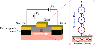
Towards realizations of quantum information processors, a variety of physical systems have been proposed and intensively investigated. In particular, solid-state devices with the quantum bits (qubits) realized by the spins of electrons confined in quantum dots in semiconductors ref:QdotTheories ; ref:Qdots ; ref:QdotsRMP are supposed to be promising in terms of its compatibility with existing semiconductor technology. Among them, vertically stacked self-assembled InAs quantum dots have advantage of strong confinement of electrons which allows high temperature operation of the order of 1K1K1\,\text{K} as opposed to mK in confined 2DEG system by Schottky electrode.ref:Qdots ; ref:QdotsRMP Thus, we have proposed and have been investigating, from both experimental and theoretical aspects, a system with vertically stacked self-assembled InAs dots buried in AlInAs barrier layer in adjacent to the channel of a spin field-effect transistor (FET) (see Fig. 1).ref:qdot-PHYE ; ref:KashiwadaYoh-JCG2007
Refer to caption
Figure 1: (Color online) Spin FET embedded with quantum dots.

For quantum information processing, one should be able to perform initialization, quantum gate operations, and readout of the qubits.ref:DiVincenzoCriteria In the proposed setup depicted in Fig. 1, the qubits evolve under the interactions with the neighboring qubits and each of them would be rotated via electric spin resonance (ESR). Furthermore, it is possible to measure repeatedly the state of the spin of the electron in the edge quantum dot, just above the channel of the FET, by making use of the “spin-blockade effect,” as will be recalled in Sec. II.ref:qdot-PHYE ; ref:KashiwadaYoh-JCG2007

Although the other qubits than the one on the edge is not directly accessible by the proposed measurement scheme, one can still perform useful operations on the chain of qubits. Multiple qubits can be initialized via repeated measurements only on the edge qubits,ref:qpfe ; ref:qdot-PHYE and an entanglement generation was discussed.ref:qdot-PHYE In the present article, we show that the state tomography (or the state reconstruction) is also available.

The determination of the quantum state is a highly nontrivial problem.ref:StateEstimationMISC A wave function, or more generally a density operator, of the state of a quantum system is not an observable and cannot be measured directly. From a practical point of view, one can see the state only through measurable quantities. In order to gain full information on the state of an N𝑁N-level system, a list of the measured values (expectation values) of N21superscript𝑁21N^{2}-1 independent observables is required, with which all the matrix elements of its density matrix are reconstructed and the tomography of the state is accomplished.

The state tomography has been carried out for a variety of physical systems to analyze experiments.ref:TomoPhoton ; ref:TomoWigner ; ref:TomoAtom ; ref:NMR ; ref:TomoElecNucl2004 ; ref:TomoSuper ; ref:TomoQdot ; ref:TomoC60 We are going to discuss the state tomography in the present setup. One can measure only the edge qubit; still, it is possible to reconstruct the state of the whole chain of the qubits.

II Spin FET Embedded with Quantum Dots

The proposed device is illustrated in Fig. 1.ref:qdot-PHYE ; ref:KashiwadaYoh-JCG2007 A series of quantum dots is embedded in the FET structure, just above the channel. A single electron is confined in each quantum dot and quantum information is encoded on its spin states, |ket|{\uparrow}\rangle and |ket|{\downarrow}\rangle. Such a situation where only a single electron is stored in each dot is realized by properly adjusting the gate voltage VGsubscript𝑉GV_{\text{G}}.ref:QdotsRMP ; ref:QdotsHoneycomb Each qubit would be rotated via ESR to perform single-qubit operations, and the qubits are entangled by the evolution under the interactions between the neighboring qubits.

The FET structure aims at measuring the spin state of the electron confined in the edge quantum dot X. Notice first that one can detect the injection of an electron from the channel into the edge dot X by looking at the channel (source-drain) current IDsubscript𝐼DI_{\text{D}} as a function of the gate voltage VGsubscript𝑉GV_{\text{G}}. As the gate voltage VGsubscript𝑉GV_{\text{G}} is increased, the channel current IDsubscript𝐼DI_{\text{D}} increases. But if an electron tunnels from the channel into the edge dot in the meanwhile, the edge dot is charged and the channel current is suppressed. As a result, the channel current IDsubscript𝐼DI_{\text{D}} drops down and exhibits a peak as a function of the gate voltage VGsubscript𝑉GV_{\text{G}} (Coulomb-blockade effect). Suppose now that the channel electrons are spin polarized in a definite spin state, say |ket|{\uparrow}\rangle. When the edge electron is in the state |ket|{\downarrow}\rangle, a channel electron in |ket|{\uparrow}\rangle can tunnel into the edge dot at a certain gate voltage VGsubscript𝑉GV_{\text{G}}, but, on the contrary, when the edge electron is in |ket|{\uparrow}\rangle, the channel electron is not allowed to enter there due to Pauli’s exclusion principle. Therefore, if the polarized channel current IDsubscript𝐼DI_{\text{D}} drops down as the gate voltage VGsubscript𝑉GV_{\text{G}} is increased, one recognizes that the edge electron is in |XsubscriptketX|{\downarrow}\rangle_{\text{X}}, while the growth of IDsubscript𝐼DI_{\text{D}} indicates that the edge electron is in |XsubscriptketX|{\uparrow}\rangle_{\text{X}}. In this way, one can measure the spin state of the edge qubit X. We call it “spin-blockade measurement.”ref:qdot-PHYE ; ref:KashiwadaYoh-JCG2007

The feasibility of the present system is discussed in Ref. ref:KashiwadaYoh-JCG2007, : (i) the selective access to each individual qubit via ESR becomes possible by slightly modifying the compound ratio x𝑥x of the In1xGaxAssubscriptIn1𝑥subscriptGa𝑥As\text{In}_{1-x}\text{Ga}_{x}\text{As} quantum dot, since the g𝑔g factor of the electron in a dot is altered in this way ref:gfactorArakawa and the ESR absorption spectra of the electrons in different dots can be separated; (ii) the strength of the exchange interaction energy between qubits and the corresponding characteristic time scale are estimated, showing the feasibility; (iii) the modulation of the channel current by single electron charging in a quantum dot adjacent to the channel has been demonstrated in a trial structure with a single layer of quantum dot, with unpolarized channel current. Spin-polarized channel will be available by replacing the normal metal electrode with a ferromagnet, candidate materials for which are being intensively investigated: see Ref. ref:YohFerhat, . Spin decoherence time has been reported to be 2ns2ns2\,\text{ns} for InAs self-assembled quantum dots,ref:DecoInAs while the spin-flipping time is estimated to be 50ps50ps50\,\text{ps}.ref:KashiwadaYoh-JCG2007

One of the remarkable features of the spin-blockade measurement is that one can measure |XsubscriptketX|{\uparrow}\rangle_{\text{X}} repeatedly. Although one is allowed to measure only the edge qubit X, this feature enables one to perform useful operations on the chain of qubits. The initialization of multiple qubits via repeated measurements on the edge qubit and an entanglement generation are discussed in Refs. ref:qdot-PHYE, and ref:qpfe, . Furthermore, the present article clarifies that the tomography of the state of the whole qubits X+A+B+\cdots is also possible via the spin-blockade measurements only on the edge qubit X.

III The Idea

In the proposed setup, it is possible to measure the state |XsubscriptketX|{\uparrow}\rangle_{\text{X}} of the edge qubit X. But at the same time, the measurement of |XsubscriptketX|{\downarrow}\rangle_{\text{X}} implies that a channel electron in |ket|{\uparrow}\rangle has been injected into the edge dot and the edge qubit X has been destroyed. Furthermore, other qubits than X are out of the reach of the spin-blockade measurement. Still, there is a way to get the full information about the state of the whole chain of the qubits.

To measure different states of X from |XsubscriptketX|{\uparrow}\rangle_{\text{X}} without loosing it by the injection of a channel electron, we apply a spin rotation just before a spin-blockade measurement. For instance, finding X in |XsubscriptketX|{\uparrow}\rangle_{\text{X}} just after rotating X by the angle π/2𝜋2\pi/2 around the y𝑦y axis is essentially the measurement of the spin X oriented in the x𝑥x direction [a superposed state (|X+|X)/2subscriptketXsubscriptketX2(|{\uparrow}\rangle_{\text{X}}+|{\downarrow}\rangle_{\text{X}})/\sqrt{2}] before the rotation. In this way, it is possible to measure any state of X.

The idea for getting information about the states of other qubits than X is to make use of the entangling dynamics of the chain of the qubits and the collapse of the state by the measurement on X. Although we are allowed to measure only X, such measurement would reflect the state of the other qubits due to the entanglement between X and the rest.

The strategy for the state tomography of the whole chain of the qubits is therefore the following. The qubits X+A+B+\cdots evolve, from a given state ϱitalic-ϱ\varrho to be reconstructed, under the action of the Hamiltonian

H=gXA𝝈(X)𝝈(A)+gAB𝝈(A)𝝈(B)+,𝐻subscript𝑔XAsuperscript𝝈(X)superscript𝝈(A)subscript𝑔ABsuperscript𝝈(A)superscript𝝈(B)H=g_{\text{XA}}\bm{\sigma}^{\text{(X)}}\cdot\bm{\sigma}^{\text{(A)}}+g_{\text{AB}}\bm{\sigma}^{\text{(A)}}\cdot\bm{\sigma}^{\text{(B)}}+\cdots, (1)

where 𝝈(Q)superscript𝝈(Q)\bm{\sigma}^{\text{(Q)}} represents the spin operator of qubit Q(=X,A,B,)\text{Q}\,(=\text{X},\text{A},\text{B},\ldots). During the evolution, we rotate some qubits and measure |XsubscriptketX|{\uparrow}\rangle_{\text{X}} a few times at definite timings according to a certain recipe. We prepare the same initial state ϱitalic-ϱ\varrho and perform such a fixed sequence of operations many times to obtain the probability for every measurement in the sequence to find X in the state |XsubscriptketX|{\uparrow}\rangle_{\text{X}}. (Notice that the measurement at the end of a sequence can be |XsubscriptketX|{\downarrow}\rangle_{\text{X}}, since we do not need to proceed further.)

Consider, for instance, the following series of operations: (rotation of X by an angle θ𝜃\theta around the x𝑥x axis) \to (wait for time τ𝜏\tau) \to (measurement of |XsubscriptketX|{\uparrow}\rangle_{\text{X}}) \to \cdots \to (measurement of |XsubscriptketX|{\downarrow}\rangle_{\text{X}}). The probability of getting the relevant result at every measurement implemented in the series is given by

p𝑝\displaystyle p =Tr{PPU(τ)Rx(X)(θ)ϱRx(X)†(θ)U(τ)PP}absentTrsubscript𝑃subscript𝑃𝑈𝜏superscriptsubscript𝑅𝑥(X)𝜃italic-ϱsuperscriptsubscript𝑅𝑥(X)†𝜃superscript𝑈𝜏subscript𝑃subscript𝑃\displaystyle=\mathop{\text{Tr}}\nolimits\{P_{\downarrow}\cdots P_{\uparrow}U(\tau)R_{x}^{\text{(X)}}(\theta)\varrho R_{x}^{\text{(X)\textdagger}}(\theta)U^{\dagger}(\tau)P_{\uparrow}\cdots P_{\downarrow}\}
=Tr{ϱ[Rx(X)†(θ)U(τ)PPPU(τ)Rx(X)(θ)]},absentTritalic-ϱdelimited-[]superscriptsubscript𝑅𝑥(X)†𝜃superscript𝑈𝜏subscript𝑃subscript𝑃subscript𝑃𝑈𝜏superscriptsubscript𝑅𝑥(X)𝜃\displaystyle=\mathop{\text{Tr}}\nolimits\{\varrho[R_{x}^{\text{(X)\textdagger}}(\theta)U^{\dagger}(\tau)P_{\uparrow}\cdots P_{\downarrow}\cdots P_{\uparrow}U(\tau)R_{x}^{\text{(X)}}(\theta)]\}, (2)

where Ri(Q)(θ)=ei2θσi(Q)superscriptsubscript𝑅𝑖(Q)𝜃superscript𝑒𝑖2𝜃superscriptsubscript𝜎𝑖(Q)R_{i}^{\text{(Q)}}(\theta)=e^{-\frac{i}{2}\theta\sigma_{i}^{\text{(Q)}}} is the operator that rotates qubit Q(=X,A,B,)\text{Q}\,(=\text{X},\text{A},\text{B},\ldots) by an angle θ𝜃\theta around the i(=x,y)i\,(=x,y) axis, P()=|()X()|P_{{\uparrow}({\downarrow})}=|{{\uparrow}({\downarrow})}\rangle_{\text{X}}\langle{{\uparrow}({\downarrow})}| is the projection operator that represents the measurement of |()X|{{\uparrow}({\downarrow})}\rangle_{\text{X}}, and U(τ)=eiHτ𝑈𝜏superscript𝑒𝑖𝐻𝜏U(\tau)=e^{-iH\tau} is the time-evolution operator between two operations and entangles the chain of the qubits.

This is the quantity that we can measure in the present system. It can be viewed as the expectation value p=Tr{ϱ𝒪}𝑝Tritalic-ϱ𝒪p=\mathop{\text{Tr}}\nolimits\{\varrho\mathcal{O}\} of a Hermitian operator 𝒪𝒪\mathcal{O} in the relevant state ϱitalic-ϱ\varrho, where 𝒪𝒪\mathcal{O} consists of Psubscript𝑃P_{\uparrow}, U(τ)𝑈𝜏U(\tau), Rx(X)(θ)superscriptsubscript𝑅𝑥X𝜃R_{x}^{(\text{X})}(\theta), and so on. Therefore, by suitably arranging the sequences of the operations, we can collect the sufficient number (4M1superscript4𝑀14^{M}-1 for an M𝑀M-qubit system) of expectation values of linearly independent operators that allow us to reconstruct the given state ϱitalic-ϱ\varrho.

Table 1: Fifteen linearly independent sequences of operations sufficient to reconstruct a state of two qubits. g=gXA𝑔subscript𝑔XAg=g_{\text{XA}} is the coupling constant between the two qubits.
Probs. Sequences of Operations
p()(1)subscriptsuperscript𝑝1absentp^{(1)}_{{\uparrow}({\downarrow})} PU(π4g)P()subscript𝑃𝑈𝜋4𝑔subscript𝑃absentP_{\uparrow}\to U(\frac{\pi}{4g})\to P_{{\uparrow}({\downarrow})}
p(2)subscriptsuperscript𝑝2p^{(2)}_{\downarrow} U(π4g)PU(π4g)P𝑈𝜋4𝑔subscript𝑃𝑈𝜋4𝑔subscript𝑃U(\frac{\pi}{4g})\to P_{\uparrow}\to U(\frac{\pi}{4g})\to P_{\downarrow}
p(3)subscriptsuperscript𝑝3p^{(3)}_{\uparrow} Ry(π)PU(π4g)Psubscript𝑅𝑦𝜋subscript𝑃𝑈𝜋4𝑔subscript𝑃R_{y}(\pi)\to P_{\uparrow}\to U(\frac{\pi}{4g})\to P_{\uparrow}
p()(4)subscriptsuperscript𝑝4absentp^{(4)}_{{\uparrow}({\downarrow})} PU(π4g)Ry(π2)P()subscript𝑃𝑈𝜋4𝑔subscript𝑅𝑦𝜋2subscript𝑃absentP_{\uparrow}\to U(\frac{\pi}{4g})\to R_{y}(\frac{\pi}{2})\to P_{{\uparrow}({\downarrow})}
p()(5)subscriptsuperscript𝑝5absentp^{(5)}_{{\uparrow}({\downarrow})} PU(π4g)Rx(π2)P()subscript𝑃𝑈𝜋4𝑔subscript𝑅𝑥𝜋2subscript𝑃absentP_{\uparrow}\to U(\frac{\pi}{4g})\to R_{x}(\frac{\pi}{2})\to P_{{\uparrow}({\downarrow})}
p()(6)subscriptsuperscript𝑝6absentp^{(6)}_{{\uparrow}({\downarrow})} U(π4g)PU(π4g)Ry(π2)P()𝑈𝜋4𝑔subscript𝑃𝑈𝜋4𝑔subscript𝑅𝑦𝜋2subscript𝑃absentU(\frac{\pi}{4g})\to P_{\uparrow}\to U(\frac{\pi}{4g})\to R_{y}(\frac{\pi}{2})\to P_{{\uparrow}({\downarrow})}
p()(7)subscriptsuperscript𝑝7absentp^{(7)}_{{\uparrow}({\downarrow})} U(π4g)PU(π4g)Rx(π2)P()𝑈𝜋4𝑔subscript𝑃𝑈𝜋4𝑔subscript𝑅𝑥𝜋2subscript𝑃absentU(\frac{\pi}{4g})\to P_{\uparrow}\to U(\frac{\pi}{4g})\to R_{x}(\frac{\pi}{2})\to P_{{\uparrow}({\downarrow})}
p()(8)subscriptsuperscript𝑝8absentp^{(8)}_{{\uparrow}({\downarrow})} Ry(π)U(π4g)PU(π4g)Ry(π2)P()subscript𝑅𝑦𝜋𝑈𝜋4𝑔subscript𝑃𝑈𝜋4𝑔subscript𝑅𝑦𝜋2subscript𝑃absentR_{y}(\pi)\to U(\frac{\pi}{4g})\to P_{\uparrow}\to U(\frac{\pi}{4g})\to R_{y}(\frac{\pi}{2})\to P_{{\uparrow}({\downarrow})}
p()(9)subscriptsuperscript𝑝9absentp^{(9)}_{{\uparrow}({\downarrow})} Ry(π)U(π4g)PU(π4g)Rx(π2)P()subscript𝑅𝑦𝜋𝑈𝜋4𝑔subscript𝑃𝑈𝜋4𝑔subscript𝑅𝑥𝜋2subscript𝑃absentR_{y}(\pi)\to U(\frac{\pi}{4g})\to P_{\uparrow}\to U(\frac{\pi}{4g})\to R_{x}(\frac{\pi}{2})\to P_{{\uparrow}({\downarrow})}
p()(10)subscriptsuperscript𝑝10absentp^{(10)}_{{\uparrow}({\downarrow})} Ry(π)PU(π4g)Ry(π2)P()subscript𝑅𝑦𝜋subscript𝑃𝑈𝜋4𝑔subscript𝑅𝑦𝜋2subscript𝑃absentR_{y}(\pi)\to P_{\uparrow}\to U(\frac{\pi}{4g})\to R_{y}(\frac{\pi}{2})\to P_{{\uparrow}({\downarrow})}
p()(11)subscriptsuperscript𝑝11absentp^{(11)}_{{\uparrow}({\downarrow})} Ry(π)PU(π4g)Rx(π2)P()subscript𝑅𝑦𝜋subscript𝑃𝑈𝜋4𝑔subscript𝑅𝑥𝜋2subscript𝑃absentR_{y}(\pi)\to P_{\uparrow}\to U(\frac{\pi}{4g})\to R_{x}(\frac{\pi}{2})\to P_{{\uparrow}({\downarrow})}
p()(12)subscriptsuperscript𝑝12absentp^{(12)}_{{\uparrow}({\downarrow})} Ry(π2)PU(π4g)P()subscript𝑅𝑦𝜋2subscript𝑃𝑈𝜋4𝑔subscript𝑃absentR_{y}(\frac{\pi}{2})\to P_{\uparrow}\to U(\frac{\pi}{4g})\to P_{{\uparrow}({\downarrow})}
p()(13)subscriptsuperscript𝑝13absentp^{(13)}_{{\uparrow}({\downarrow})} Rx(π2)PU(π4g)P()subscript𝑅𝑥𝜋2subscript𝑃𝑈𝜋4𝑔subscript𝑃absentR_{x}(\frac{\pi}{2})\to P_{\uparrow}\to U(\frac{\pi}{4g})\to P_{{\uparrow}({\downarrow})}
p()(14)subscriptsuperscript𝑝14absentp^{(14)}_{{\uparrow}({\downarrow})} Ry(π2)PU(π4g)Rx(π2)P()subscript𝑅𝑦𝜋2subscript𝑃𝑈𝜋4𝑔subscript𝑅𝑥𝜋2subscript𝑃absentR_{y}(\frac{\pi}{2})\to P_{\uparrow}\to U(\frac{\pi}{4g})\to R_{x}(\frac{\pi}{2})\to P_{{\uparrow}({\downarrow})}
p()(15)subscriptsuperscript𝑝15absentp^{(15)}_{{\uparrow}({\downarrow})} Rx(π2)PU(π4g)Ry(π2)P()subscript𝑅𝑥𝜋2subscript𝑃𝑈𝜋4𝑔subscript𝑅𝑦𝜋2subscript𝑃absentR_{x}(\frac{\pi}{2})\to P_{\uparrow}\to U(\frac{\pi}{4g})\to R_{y}(\frac{\pi}{2})\to P_{{\uparrow}({\downarrow})}
Table 2: Reconstruction of the two-qubit state ϱitalic-ϱ\varrho from the probabilities p()(n)subscriptsuperscript𝑝𝑛absentp^{(n)}_{{\uparrow}({\downarrow})} obtained by the sequences of operations listed in Table 1. Here, |=|X|A|{\uparrow\downarrow}\rangle=|{\uparrow}\rangle_{\text{X}}|{\downarrow}\rangle_{\text{A}}, etc.
|ϱ|=\langle{\uparrow\uparrow}|\varrho|{\uparrow\uparrow}\rangle={} p(1)subscriptsuperscript𝑝1p^{(1)}_{\uparrow},   |ϱ|=p(3)\langle{\downarrow\downarrow}|\varrho|{\downarrow\downarrow}\rangle=p^{(3)}_{\uparrow}
|ϱ|=\langle{\uparrow\downarrow}|\varrho|{\uparrow\downarrow}\rangle={} p(1)subscriptsuperscript𝑝1p^{(1)}_{\downarrow},   |ϱ|=p(2)\langle{\downarrow\uparrow}|\varrho|{\downarrow\uparrow}\rangle=p^{(2)}_{\downarrow}
|ϱ|=\langle{\uparrow\uparrow}|\varrho|{\uparrow\downarrow}\rangle={} 12(-\frac{1}{2}\,\Bigl{(} p(4)p(4))i2(p(5)p(5))p^{(4)}_{\uparrow}-p^{(4)}_{\downarrow}\Bigr{)}-\frac{i}{2}\,\Bigl{(}p^{(5)}_{\uparrow}-p^{(5)}_{\downarrow}\Bigr{)}
|ϱ|=\langle{\uparrow\downarrow}|\varrho|{\uparrow\uparrow}\rangle={} 12(-\frac{1}{2}\,\Bigl{(} p(4)p(4))+i2(p(5)p(5))p^{(4)}_{\uparrow}-p^{(4)}_{\downarrow}\Bigr{)}+\frac{i}{2}\,\Bigl{(}p^{(5)}_{\uparrow}-p^{(5)}_{\downarrow}\Bigr{)}
|ϱ|=\langle{\uparrow\uparrow}|\varrho|{\downarrow\uparrow}\rangle={} 12(-\frac{1}{2}\,\Bigl{(} p(6)p(6))i2(p(7)p(7))p^{(6)}_{\uparrow}-p^{(6)}_{\downarrow}\Bigr{)}-\frac{i}{2}\,\Bigl{(}p^{(7)}_{\uparrow}-p^{(7)}_{\downarrow}\Bigr{)}
|ϱ|=\langle{\downarrow\uparrow}|\varrho|{\uparrow\uparrow}\rangle={} 12(-\frac{1}{2}\,\Bigl{(} p(6)p(6))+i2(p(7)p(7))p^{(6)}_{\uparrow}-p^{(6)}_{\downarrow}\Bigr{)}+\frac{i}{2}\,\Bigl{(}p^{(7)}_{\uparrow}-p^{(7)}_{\downarrow}\Bigr{)}
|ϱ|=\langle{\downarrow\downarrow}|\varrho|{\uparrow\downarrow}\rangle={} 12(\frac{1}{2}\,\Bigl{(} p(8)p(8))+i2(p(9)p(9))p^{(8)}_{\uparrow}-p^{(8)}_{\downarrow}\Bigr{)}+\frac{i}{2}\,\Bigl{(}p^{(9)}_{\uparrow}-p^{(9)}_{\downarrow}\Bigr{)}
|ϱ|=\langle{\uparrow\downarrow}|\varrho|{\downarrow\downarrow}\rangle={} 12(\frac{1}{2}\,\Bigl{(} p(8)p(8))i2(p(9)p(9))p^{(8)}_{\uparrow}-p^{(8)}_{\downarrow}\Bigr{)}-\frac{i}{2}\,\Bigl{(}p^{(9)}_{\uparrow}-p^{(9)}_{\downarrow}\Bigr{)}
|ϱ|=\langle{\downarrow\downarrow}|\varrho|{\downarrow\uparrow}\rangle={} 12(\frac{1}{2}\,\Bigl{(} p(10)p(10))+i2(p(11)p(11))p^{(10)}_{\uparrow}-p^{(10)}_{\downarrow}\Bigr{)}+\frac{i}{2}\,\Bigl{(}p^{(11)}_{\uparrow}-p^{(11)}_{\downarrow}\Bigr{)}
|ϱ|=\langle{\downarrow\uparrow}|\varrho|{\downarrow\downarrow}\rangle={} 12(\frac{1}{2}\,\Bigl{(} p(10)p(10))i2(p(11)p(11))p^{(10)}_{\uparrow}-p^{(10)}_{\downarrow}\Bigr{)}-\frac{i}{2}\,\Bigl{(}p^{(11)}_{\uparrow}-p^{(11)}_{\downarrow}\Bigr{)}
|ϱ|=\langle{\uparrow\uparrow}|\varrho|{\downarrow\downarrow}\rangle={} 14(\frac{1}{4}\,\Bigl{(} σx(X)σx(A)σy(X)σy(A)delimited-⟨⟩superscriptsubscript𝜎𝑥(X)superscriptsubscript𝜎𝑥(A)delimited-⟨⟩superscriptsubscript𝜎𝑦(X)superscriptsubscript𝜎𝑦(A)\langle\sigma_{x}^{\text{(X)}}\sigma_{x}^{\text{(A)}}\rangle-\langle\sigma_{y}^{\text{(X)}}\sigma_{y}^{\text{(A)}}\rangle
iσx(X)σy(A)iσy(X)σx(A)){}-i\langle\sigma_{x}^{\text{(X)}}\sigma_{y}^{\text{(A)}}\rangle-i\langle\sigma_{y}^{\text{(X)}}\sigma_{x}^{\text{(A)}}\rangle\Bigr{)}
|ϱ|=\langle{\downarrow\downarrow}|\varrho|{\uparrow\uparrow}\rangle={} 14(\frac{1}{4}\,\Bigl{(} σx(X)σx(A)σy(X)σy(A)delimited-⟨⟩superscriptsubscript𝜎𝑥(X)superscriptsubscript𝜎𝑥(A)delimited-⟨⟩superscriptsubscript𝜎𝑦(X)superscriptsubscript𝜎𝑦(A)\langle\sigma_{x}^{\text{(X)}}\sigma_{x}^{\text{(A)}}\rangle-\langle\sigma_{y}^{\text{(X)}}\sigma_{y}^{\text{(A)}}\rangle
+iσx(X)σy(A)+iσy(X)σx(A)){}+i\langle\sigma_{x}^{\text{(X)}}\sigma_{y}^{\text{(A)}}\rangle+i\langle\sigma_{y}^{\text{(X)}}\sigma_{x}^{\text{(A)}}\rangle\Bigr{)}
|ϱ|=\langle{\uparrow\downarrow}|\varrho|{\downarrow\uparrow}\rangle={} 14(\frac{1}{4}\,\Bigl{(} σx(X)σx(A)+σy(X)σy(A)delimited-⟨⟩superscriptsubscript𝜎𝑥(X)superscriptsubscript𝜎𝑥(A)delimited-⟨⟩superscriptsubscript𝜎𝑦(X)superscriptsubscript𝜎𝑦(A)\langle\sigma_{x}^{\text{(X)}}\sigma_{x}^{\text{(A)}}\rangle+\langle\sigma_{y}^{\text{(X)}}\sigma_{y}^{\text{(A)}}\rangle
+iσx(X)σy(A)iσy(X)σx(A)){}+i\langle\sigma_{x}^{\text{(X)}}\sigma_{y}^{\text{(A)}}\rangle-i\langle\sigma_{y}^{\text{(X)}}\sigma_{x}^{\text{(A)}}\rangle\Bigr{)}
|ϱ|=\langle{\downarrow\uparrow}|\varrho|{\uparrow\downarrow}\rangle={} 14(\frac{1}{4}\,\Bigl{(} σx(X)σx(A)+σy(X)σy(A)delimited-⟨⟩superscriptsubscript𝜎𝑥(X)superscriptsubscript𝜎𝑥(A)delimited-⟨⟩superscriptsubscript𝜎𝑦(X)superscriptsubscript𝜎𝑦(A)\langle\sigma_{x}^{\text{(X)}}\sigma_{x}^{\text{(A)}}\rangle+\langle\sigma_{y}^{\text{(X)}}\sigma_{y}^{\text{(A)}}\rangle
iσx(X)σy(A)+iσy(X)σx(A)){}-i\langle\sigma_{x}^{\text{(X)}}\sigma_{y}^{\text{(A)}}\rangle+i\langle\sigma_{y}^{\text{(X)}}\sigma_{x}^{\text{(A)}}\rangle\Bigr{)}
σx(X)σx(A)=delimited-⟨⟩superscriptsubscript𝜎𝑥(X)superscriptsubscript𝜎𝑥(A)absent\langle\sigma_{x}^{\text{(X)}}\sigma_{x}^{\text{(A)}}\rangle={} 2(2\,\Bigl{(} p(12)p(12))+σx(A)p^{(12)}_{\uparrow}-p^{(12)}_{\downarrow}\Bigr{)}+\langle\sigma_{x}^{\text{(A)}}\rangle
σy(X)σy(A)=delimited-⟨⟩superscriptsubscript𝜎𝑦(X)superscriptsubscript𝜎𝑦(A)absent\langle\sigma_{y}^{\text{(X)}}\sigma_{y}^{\text{(A)}}\rangle={} 2(2\,\Bigl{(} p(13)p(13))σy(A)p^{(13)}_{\uparrow}-p^{(13)}_{\downarrow}\Bigr{)}-\langle\sigma_{y}^{\text{(A)}}\rangle
σx(X)σy(A)=delimited-⟨⟩superscriptsubscript𝜎𝑥(X)superscriptsubscript𝜎𝑦(A)absent\langle\sigma_{x}^{\text{(X)}}\sigma_{y}^{\text{(A)}}\rangle={} 2(-2\,\Bigl{(} p(14)p(14))+σy(A)p^{(14)}_{\uparrow}-p^{(14)}_{\downarrow}\Bigr{)}+\langle\sigma_{y}^{\text{(A)}}\rangle
σy(X)σx(A)=delimited-⟨⟩superscriptsubscript𝜎𝑦(X)superscriptsubscript𝜎𝑥(A)absent\langle\sigma_{y}^{\text{(X)}}\sigma_{x}^{\text{(A)}}\rangle={} 2(-2\,\Bigl{(} p(15)p(15))σx(A)p^{(15)}_{\uparrow}-p^{(15)}_{\downarrow}\Bigr{)}-\langle\sigma_{x}^{\text{(A)}}\rangle
σx(A)=delimited-⟨⟩superscriptsubscript𝜎𝑥(A)absent\langle\sigma_{x}^{\text{(A)}}\rangle={} (-\Bigl{(} p(4)p(4))+(p(10)p(10))p^{(4)}_{\uparrow}-p^{(4)}_{\downarrow}\Bigr{)}+\Bigl{(}p^{(10)}_{\uparrow}-p^{(10)}_{\downarrow}\Bigr{)}
σy(A)=delimited-⟨⟩superscriptsubscript𝜎𝑦(A)absent\langle\sigma_{y}^{\text{(A)}}\rangle={} ((\Bigl{(} p(5)p(5))(p(11)p(11))p^{(5)}_{\uparrow}-p^{(5)}_{\downarrow}\Bigr{)}-\Bigl{(}p^{(11)}_{\uparrow}-p^{(11)}_{\downarrow}\Bigr{)}

Let us demonstrate how the above procedure works in the simplest case, for two qubits X+A. Fifteen linearly independent sequences of operations that are sufficient to reconstruct a two-qubit state ϱitalic-ϱ\varrho are listed in Table 1, where Ri(θ)=Ri(X)(θ)Ri(A)(θ)subscript𝑅𝑖𝜃superscriptsubscript𝑅𝑖(X)𝜃superscriptsubscript𝑅𝑖(A)𝜃R_{i}(\theta)=R_{i}^{\text{(X)}}(\theta)R_{i}^{\text{(A)}}(\theta) is a “global” rotation, which rotates both X and A at the same time (we can also construct a recipe with “local” rotations, which act separately on X or A). Note that p(n)superscriptsubscript𝑝𝑛p_{\uparrow}^{(n)} and p(n)superscriptsubscript𝑝𝑛p_{\downarrow}^{(n)} are obtained simultaneously, by a common ensemble of experimental data collected for the n𝑛nth sequence of operations. By substituting the probabilities p()(n)superscriptsubscript𝑝absent𝑛p_{{\uparrow}({\downarrow})}^{(n)} measured for the sequences of operations into the formulas listed in Table 2, all of the 161616 matrix elements of the two-qubit state ϱitalic-ϱ\varrho are disclosed and the state ϱitalic-ϱ\varrho is reconstructed.

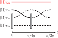
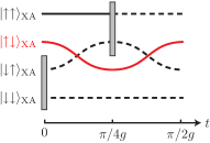
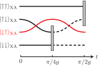
The mechanism of the tomography is understood as follows, for relatively simple cases. The curves in Fig. 2 describe the entangling dynamics according to the Hamiltonian (1). If the result of a measurement on X is “no,” two of the four components of the state of X+A are projected out. The survival through such projections corresponds to the event where every measurement in a sequence gives “yes,” and the probability of such an event rephrases how much the survived component was contained in the given initial state ϱitalic-ϱ\varrho. The sequences are designed so as to reflect all of the matrix elements of ϱitalic-ϱ\varrho, and the inversion of a linear relationship between the probabilities and the matrix elements reconstructs the given state ϱitalic-ϱ\varrho.

(a) for p(1)superscriptsubscript𝑝1p_{\uparrow}^{(1)} (b) for p(1)superscriptsubscript𝑝1p_{\downarrow}^{(1)}
Refer to caption Refer to caption
(c) for p(2)superscriptsubscript𝑝2p_{\downarrow}^{(2)}
Refer to caption
Figure 2: (Color online) Mechanism of the tomography, for the sequences of operations for (a) p(1)superscriptsubscript𝑝1p_{\uparrow}^{(1)}, (b) p(1)superscriptsubscript𝑝1p_{\downarrow}^{(1)}, and (c) p(2)superscriptsubscript𝑝2p_{\downarrow}^{(2)}. The curves describe how the components of a state evolve and entangle in time according to the Hamiltonian (1), while the “walls” represent the projective measurements on qubit X. The survived curves which are not shut off by the walls correspond to the events where every measurement gives the desired result. The probabilities of such events are nothing but the probabilities p()(n)superscriptsubscript𝑝absent𝑛p_{{\uparrow}({\downarrow})}^{(n)} for the sequences of operations and are equivalent (in the simple cases shown here) to the occupations of the survived states in the given initial state ϱitalic-ϱ\varrho, yielding its relevant matrix elements, (a) |ϱ|\langle{\uparrow\uparrow}|\varrho|{\uparrow\uparrow}\rangle, (b) |ϱ|\langle{\uparrow\downarrow}|\varrho|{\uparrow\downarrow}\rangle, and (c) |ϱ|\langle{\downarrow\uparrow}|\varrho|{\downarrow\uparrow}\rangle.

IV Partially Polarized Spin Channel

The realization of the polarized spin channel is one of the important issues to be tackled.ref:YohFerhat If the channel is only partially polarized, the fidelity of the spin-blockade measurement on X is degraded and the performance of the tomography deteriorates. Let us clarify the effect of the partially polarized spin channel on the tomographic scheme presented in the previous section.

When the spin polarization is not perfect but r𝑟r, the state of the electron in the channel would be effectively described by the density operator

ϱchsubscriptitalic-ϱch\displaystyle\varrho_{\text{ch}} =r||+1r2𝟙\displaystyle=r|{\uparrow}\rangle\langle{\uparrow}|+\frac{1-r}{2}\openone
=1+r2||+1r2||.\displaystyle=\frac{1+r}{2}|{\uparrow}\rangle\langle{\uparrow}|+\frac{1-r}{2}|{\downarrow}\rangle\langle{\downarrow}|. (3)

Due to the presence of the undesired ingredient, |||{\downarrow}\rangle\langle{\downarrow}| in (3), the confirmation of the increase in the channel current in response to the sweep of the gate voltage does not result in the pure projection ϱPϱPitalic-ϱsubscript𝑃italic-ϱsubscript𝑃\varrho\to P_{\uparrow}\varrho P_{\uparrow} but would induce

ϱ1+r2PϱP+1r2PϱP,italic-ϱ1𝑟2subscript𝑃italic-ϱsubscript𝑃1𝑟2subscript𝑃italic-ϱsubscript𝑃\varrho\to\frac{1+r}{2}P_{\uparrow}\varrho P_{\uparrow}+\frac{1-r}{2}P_{\downarrow}\varrho P_{\downarrow}, (4)

reflecting the classical mixture of the two states in (3) (with other possible non-ideal features omitted).note:Projection

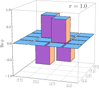
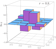
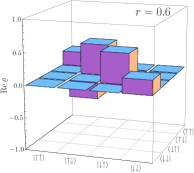
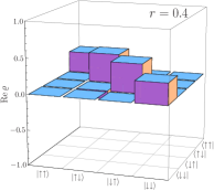
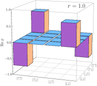
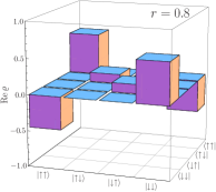
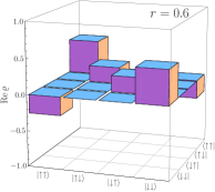
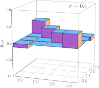
See Figs. 3 and 4, where the state reconstructions are simulated with the spin-blockade measurement with partially polarized spin channel, Eq. (4), in place of the ideal projective measurement Psubscript𝑃P_{\uparrow} in the recipe presented in Table 1.

Refer to caption Refer to caption
Figure 3: (Color online) State tomography of |Ψ=(|XA|XA)/2|{\Psi^{-}}\rangle=(|{\uparrow\downarrow}\rangle_{\text{XA}}-|{\downarrow\uparrow}\rangle_{\text{XA}})/\sqrt{2} with partially polarized spin channel. The polarization of the channel is defined by r=(NN)/(N+N)𝑟subscript𝑁subscript𝑁subscript𝑁subscript𝑁r=(N_{\uparrow}-N_{\downarrow})/(N_{\uparrow}+N_{\downarrow}) with N()subscript𝑁absentN_{{\uparrow}(\downarrow)} the number of spins in the |()|{{\uparrow}(\downarrow)}\rangle state in the channel.
Refer to caption Refer to caption
Figure 4: (Color online) State tomography of |Φ=(|XA|XA)/2|{\Phi^{-}}\rangle=(|{\uparrow\uparrow}\rangle_{\text{XA}}-|{\downarrow\downarrow}\rangle_{\text{XA}})/\sqrt{2} with partially polarized spin channel.

We have considered the imperfection of the spin-blockade measurement due to the partially polarized spin channel. The present formalism [Eq. (4)] would however be applicable to other physical origins of imperfections, including imperfect Pauli blocking.ref:DecoSemicondDot The meaning of the parameter r𝑟r is just to be reinterpreted.

V Towards Multi-Qubit Systems

Towards the tomography of multiple qubits (with M3𝑀3M\geq 3), there exists a scheme applicable for an arbitrary number of qubits M𝑀M. Here is the recipe: we consider four sequences of operations

Rθ0φ0(X)P[U(τ)Rθφ(X)P]N1R_{\theta_{0}\varphi_{0}}^{\text{(X)}}\to P_{\uparrow}\,[\to U(\tau)\to R_{\theta\varphi}^{\text{(X)}}\to P_{\uparrow}]^{N-1} (5)

with (θ0,φ0)=(0,0),(π,0),(π/2,0),(π/2,π/2)subscript𝜃0subscript𝜑000𝜋0𝜋20𝜋2𝜋2(\theta_{0},\varphi_{0})=(0,0),(\pi,0),(\pi/2,0),(\pi/2,\pi/2) and ND2/4𝑁superscript𝐷24N\leq D^{2}/4, where D=2M𝐷superscript2𝑀D=2^{M} is the dimension of the M𝑀M-qubit system and Rθφ(X)superscriptsubscript𝑅𝜃𝜑(X)R_{\theta\varphi}^{\text{(X)}} represents a rotation of X defined by

Rθφ(X)†|X=eiφ/2cosθ2|X+eiφ/2sinθ2|X.superscriptsubscript𝑅𝜃𝜑(X)†subscriptketXsuperscript𝑒𝑖𝜑2𝜃2subscriptketXsuperscript𝑒𝑖𝜑2𝜃2subscriptketXR_{\theta\varphi}^{\text{(X)\textdagger}}|{\uparrow}\rangle_{\text{X}}=e^{-i\varphi/2}\cos\frac{\theta}{2}|{\uparrow}\rangle_{\text{X}}+e^{i\varphi/2}\sin\frac{\theta}{2}|{\downarrow}\rangle_{\text{X}}. (6)

Let pθ0φ0(N)subscript𝑝subscript𝜃0subscript𝜑0𝑁p_{\theta_{0}\varphi_{0}}(N) denote the probability of finding X in |XsubscriptketX|{\uparrow}\rangle_{\text{X}} successively N𝑁N times up to the N𝑁Nth measurement, which is given by

pθ0φ0(N)subscript𝑝subscript𝜃0subscript𝜑0𝑁\displaystyle p_{\theta_{0}\varphi_{0}}(N) =Tr{[PRθφ(X)U(τ)]N1PRθ0φ0(X)ϱ\displaystyle=\mathop{\text{Tr}}\nolimits\{[P_{\uparrow}R_{\theta\varphi}^{\text{(X)}}U(\tau)]^{N-1}P_{\uparrow}R_{\theta_{0}\varphi_{0}}^{\text{(X)}}\varrho
×Rθ0φ0(X)†P[U(τ)Rθφ(X)†P]N1}\displaystyle\qquad\qquad{}\times R_{\theta_{0}\varphi_{0}}^{\text{(X)\textdagger}}P_{\uparrow}[U^{\dagger}(\tau)R_{\theta\varphi}^{\text{(X)\textdagger}}P_{\uparrow}]^{N-1}\}
=TrAB…{[Vθφ(τ)]N1ϱθ0φ0[Vθφ(τ)]N1}absentsubscriptTrAB…superscriptdelimited-[]subscript𝑉𝜃𝜑𝜏𝑁1subscriptitalic-ϱsubscript𝜃0subscript𝜑0superscriptdelimited-[]superscriptsubscript𝑉𝜃𝜑𝜏𝑁1\displaystyle=\mathop{\text{Tr}}\nolimits_{\text{AB\ldots}}\{[V_{\theta\varphi}(\tau)]^{N-1}\varrho_{\theta_{0}\varphi_{0}}[V_{\theta\varphi}^{\dagger}(\tau)]^{N-1}\} (7)

with

Vθφ(τ)=|Rθφ(X)U(τ)|XX,\displaystyle V_{\theta\varphi}(\tau)={}_{\text{X}}\langle{\uparrow}|R_{\theta\varphi}^{\text{(X)}}U(\tau)|{\uparrow}\rangle_{\text{X}}, (8a)
ϱθ0φ0=|Rθ0φ0(X)ϱRθ0φ0(X)†|XX.\displaystyle\varrho_{\theta_{0}\varphi_{0}}={}_{\text{X}}\langle{\uparrow}|R_{\theta_{0}\varphi_{0}}^{\text{(X)}}\varrho R_{\theta_{0}\varphi_{0}}^{\text{(X)\textdagger}}|{\uparrow}\rangle_{\text{X}}. (8b)

Then, such probabilities are related to the matrix elements of the given density operator ϱitalic-ϱ\varrho of X+A+B+\cdots through

(pθ0φ0(1)pθ0φ0(2)pθ0φ0(D24))=(u1|u1v1|ϱθ0φ0|v1u2|u1v1|ϱθ0φ0|v2uD2|uD2vD2|ϱθ0φ0|vD2),matrixsubscript𝑝subscript𝜃0subscript𝜑01subscript𝑝subscript𝜃0subscript𝜑02subscript𝑝subscript𝜃0subscript𝜑0superscript𝐷24matrixinner-productsubscript𝑢1subscript𝑢1quantum-operator-productsubscript𝑣1subscriptitalic-ϱsubscript𝜃0subscript𝜑0subscript𝑣1inner-productsubscript𝑢2subscript𝑢1quantum-operator-productsubscript𝑣1subscriptitalic-ϱsubscript𝜃0subscript𝜑0subscript𝑣2inner-productsubscript𝑢𝐷2subscript𝑢𝐷2quantum-operator-productsubscript𝑣𝐷2subscriptitalic-ϱsubscript𝜃0subscript𝜑0subscript𝑣𝐷2\begin{pmatrix}p_{\theta_{0}\varphi_{0}}(1)\\ p_{\theta_{0}\varphi_{0}}(2)\\ \vdots\\ p_{\theta_{0}\varphi_{0}}(\frac{D^{2}}{4})\end{pmatrix}=\mathcal{M}\begin{pmatrix}\langle u_{1}|u_{1}\rangle\langle{v_{1}}|\varrho_{\theta_{0}\varphi_{0}}|{v_{1}}\rangle\\ \langle u_{2}|u_{1}\rangle\langle{v_{1}}|\varrho_{\theta_{0}\varphi_{0}}|{v_{2}}\rangle\\ \vdots\\ \langle u_{\frac{D}{2}}|u_{\frac{D}{2}}\rangle\langle{v_{\frac{D}{2}}}|\varrho_{\theta_{0}\varphi_{0}}|{v_{\frac{D}{2}}}\rangle\end{pmatrix}, (9)

where

=(111λ1λ1λ1λ2λD2λD2(λ1λ1)2(λ1λ2)2(λD2λD2)2(λ1λ1)D241(λ1λ2)D241(λD2λD2)D241)matrix111subscript𝜆1superscriptsubscript𝜆1subscript𝜆1superscriptsubscript𝜆2subscript𝜆𝐷2superscriptsubscript𝜆𝐷2superscriptsubscript𝜆1superscriptsubscript𝜆12superscriptsubscript𝜆1superscriptsubscript𝜆22superscriptsubscript𝜆𝐷2superscriptsubscript𝜆𝐷22superscriptsubscript𝜆1superscriptsubscript𝜆1superscript𝐷241superscriptsubscript𝜆1superscriptsubscript𝜆2superscript𝐷241superscriptsubscript𝜆𝐷2superscriptsubscript𝜆𝐷2superscript𝐷241\mathcal{M}=\begin{pmatrix}1&1&\cdots&1\\ \lambda_{1}\lambda_{1}^{*}&\lambda_{1}\lambda_{2}^{*}&\cdots&\lambda_{\frac{D}{2}}\lambda_{\frac{D}{2}}^{*}\\ (\lambda_{1}\lambda_{1}^{*})^{2}&(\lambda_{1}\lambda_{2}^{*})^{2}&\cdots&(\lambda_{\frac{D}{2}}\lambda_{\frac{D}{2}}^{*})^{2}\\ \vdots&\vdots&\ddots&\vdots\\ (\lambda_{1}\lambda_{1}^{*})^{\frac{D^{2}}{4}-1}&(\lambda_{1}\lambda_{2}^{*})^{\frac{D^{2}}{4}-1}&\cdots&(\lambda_{\frac{D}{2}}\lambda_{\frac{D}{2}}^{*})^{\frac{D^{2}}{4}-1}\end{pmatrix} (10)

and

Vθφ(τ)|un=λn|un,vn|Vθφ(τ)=λnvn|.formulae-sequencesubscript𝑉𝜃𝜑𝜏ketsubscript𝑢𝑛subscript𝜆𝑛ketsubscript𝑢𝑛brasubscript𝑣𝑛subscript𝑉𝜃𝜑𝜏subscript𝜆𝑛brasubscript𝑣𝑛V_{\theta\varphi}(\tau)|{u_{n}}\rangle=\lambda_{n}|{u_{n}}\rangle,\quad\langle{v_{n}}|V_{\theta\varphi}(\tau)=\lambda_{n}\langle{v_{n}}|. (11)

The non-Hermitian operator Vθφ(τ)subscript𝑉𝜃𝜑𝜏V_{\theta\varphi}(\tau) has been assumed to be diagonalizable.ref:qpfe

The matrix \mathcal{M} in (10) is a Vandermonde matrix of order D2/4superscript𝐷24D^{2}/4, whose properties are well known.ref:IntegralTable In particular, its determinant is given by

det=(m,n)>(k,)(λmλnλkλ)subscriptproduct𝑚𝑛𝑘subscript𝜆𝑚superscriptsubscript𝜆𝑛subscript𝜆𝑘superscriptsubscript𝜆\det\mathcal{M}=\prod_{(m,n)>(k,\ell)}(\lambda_{m}\lambda_{n}^{*}-\lambda_{k}\lambda_{\ell}^{*}) (12)

and the formula for the inverse 1superscript1\mathcal{M}^{-1} is available, where (m,n)>(k,)𝑚𝑛𝑘(m,n)>(k,\ell) means Imn>Iksubscript𝐼𝑚𝑛subscript𝐼𝑘I_{mn}>I_{k\ell} with Imn=(D/2)(m1)+nsubscript𝐼𝑚𝑛𝐷2𝑚1𝑛I_{mn}=(D/2)(m-1)+n. The determinant (12) is the product of all the differences that can be formed by any pairs taken from {λmλn}subscript𝜆𝑚superscriptsubscript𝜆𝑛\{\lambda_{m}\lambda_{n}^{*}\}. It is therefore clear when it is possible to invert the relation (9) to reconstruct the density operator ϱθ0φ0subscriptitalic-ϱsubscript𝜃0subscript𝜑0\varrho_{\theta_{0}\varphi_{0}} of A+B+\cdots: the parameters τ𝜏\tau and (θ,φ)𝜃𝜑(\theta,\varphi) should be chosen so as to satisfy the conditions

{λmλnun|um0(m,n=1,,D/2),λmλnλkλfor(m,n)(k,).\begin{cases}\vskip 6.0pt plus 2.0pt minus 2.0pt\lambda_{m}\lambda_{n}^{*}\langle u_{n}|u_{m}\rangle\neq 0\ (m,n=1,\ldots,D/2),\\ \lambda_{m}\lambda_{n}^{*}\neq\lambda_{k}\lambda_{\ell}^{*}\quad\text{for}\quad(m,n)\neq(k,\ell).\end{cases} (13)

In this way, one gets a list of ϱθ0φ0subscriptitalic-ϱsubscript𝜃0subscript𝜑0\varrho_{\theta_{0}\varphi_{0}} for the four independent sets of (θ0,φ0)subscript𝜃0subscript𝜑0(\theta_{0},\varphi_{0}), which completes the tomography of the state ϱitalic-ϱ\varrho.

This scheme is quite simple and general: one simply repeats PRθφ(X)subscript𝑃superscriptsubscript𝑅𝜃𝜑(X)P_{\uparrow}R_{\theta\varphi}^{\text{(X)}} necessary times, the scheme works for an arbitrary number of qubits M𝑀M, and the conditions for the parameters are clear [Eq. (13)]. Only four independent sequences are required, irrespective of the number of qubits M𝑀M.

VI Summary

In this article, we have discussed the state tomography for a chain of qubits in the setup (Fig. 1) proposed as a possible physical realization of a quantum information processor. In this setup, only the state of the edge qubit of the chain is measurable via the spin-blockade measurement. However, the present analysis explicitly demonstrates that it is still possible to reconstruct the state of the whole chain of qubits. The idea is to make use of the entangling dynamics of the qubits, which enables one to gain information on the whole chain through the edge qubit.

Such an idea is not restricted to the current setup: there would be various physical systems in which only limited degrees of freedom are accessible in practice and similar strategies are required. The present idea would find many valuable applications.

In Sec. III, we have explicitly constructed a recipe for two qubits. We have also presented a general scheme based on repeated measurements that can be applied to an arbitrary number of qubits (Sec. V). There are, however, many other possibilities. For instance, the latter scheme requires 22(M1)superscript22𝑀12^{2(M-1)} measurements for M𝑀M qubits, i.e. 4 measurements for 2 qubits, while each sequence in Table 1 involves only 2 measurements. As mentioned in Sec. IV, the accuracy of the spin-blockade measurement relies on the polarization of the channel spins. For a partially polarized spin channel, it would be better to seek a scheme with fewer measurements. Shorter sequences of operations would be preferable also to minimize other possible errors, originating for instance from imperfect qubit rotations by ESR and decoherence during the processes.

There would exist recipes that involve only one measurement (and therefore with fewer rotations and a shorter execution time) for each sequence, but no general prescription for generating such sequences of operations is known (at least to the present authors). A possible strategy would be to generate sequences according to a certain rule anyway, to select necessary number of sequences (since too many sequences might be generated for the reconstruction of a density operator with 4M1superscript4𝑀14^{M}-1 independent matrix elements), and to check the invertibility of the relevant matrix relating the matrix elements of the target density operator to the observable data. It is desirable to clarify how to generate the optimal sequences efficiently, which remains a future subject.

Acknowledgements.
This work is partly supported by the bilateral Italian-Japanese Projects II04C1AF4E on “Quantum Information, Computation and Communication” of the Italian Ministry of Education, University and Research, and the Joint Italian-Japanese Laboratory on “Quantum Information and Computation” of the Italian Ministry for Foreign Affairs, by a Special Coordination Fund for Promoting Science and Technology from the Ministry of Education, Culture, Sports, Science and Technology, Japan, and by the Grants-in-Aid for Scientific Research (A) and (C) from the Japan Society for the Promotion of Science. Support by Japan Science and Technology Agency is also gratefully acknowledged.

References

  • (1) D. Loss and D. P. DiVincenzo, Phys. Rev. A 57, 120 (1998); B. E. Kane, Nature (London) 393, 133 (1998).
  • (2) T. Fujisawa, D. G. Austing, Y. Tokura, Y. Hirayama, and S. Tarucha, Nature (London) 419, 278 (2002); J. R. Petta, A. C. Johnson, J. M. Taylor, E. A. Laird, A. Yacoby, M. D. Lukin, C. M. Marcus, M. P. Hanson, and A. C. Gossard, Science 309, 2180 (2005); F. H. L. Koppens, C. Buizert, K. J. Tielrooij, I. T. Vink, K. C. Nowack, T. Meunier, L. P. Kouwenhoven and L. M. K. Vandersypen, Nature (London) 442, 766 (2006).
  • (3) R. Hanson, L. P. Kouwenhoven, J. R. Petta, S. Tarucha, and L. M. K. Vandersypen, Rev. Mod. Phys. 79, 1217 (2007).
  • (4) K. Yoh, K. Yuasa, and H. Nakazato, Physica E 29, 674 (2005).
  • (5) S. Kashiwada, T. Matsuda, and K. Yoh, J. Cryst. Growth 301-302, 785 (2007).
  • (6) D. P. DiVincenzo, Fortschr. Phys. 48, 771 (2000).
  • (7) H. Nakazato, M. Unoki, and K. Yuasa, Phys. Rev. A 70, 012303 (2004).
  • (8) Quantum State Estimation, edited by M. G. A. Paris and J. Řeháček (Springer, Berlin, 2004).
  • (9) P. Kok, W. J. Munro, K. Nemoto, T. C. Ralph, J. P. Dowling, and G. J. Milburn, Rev. Mod. Phys. 79, 135 (2007), and references therein.
  • (10) A. I. Lvovsky and M. G. Raymer, Rev. Mod. Phys. 81, 299 (2009), and references therein.
  • (11) H. Häffner, W. Hänsel, C. F. Roos, J. Benhelm, D. Chek-al-kar, M. Chwalla, T. Körber, U. D. Rapol, M. Riebe, P. O. Schmidt, C. Becher, O. Gühne, W. Dür, and R. Blatt, Nature (London) 438, 643 (2005).
  • (12) I. L. Chuang, N. Gershenfeld, M. G. Kubinec, and D. W. Leung, Proc. Roy. Soc. (London) A 454, 447 (1998).
  • (13) F. Jelezko, T. Gaebel, I. Popa, M. Domhan, A. Gruber, and J. Wrachtrup, Phys. Rev. Lett. 93, 130501 (2004).
  • (14) N. Katz, M. Ansmann, R. C. Bialczak, E. Lucero, R. McDermott, M. Neeley, M. Steffen, E. M. Weig, A. N. Cleland, J. M. Martinis, and A. N. Korotkov, Science 312, 1498 (2006).
  • (15) Y. Wu, X. Li, L. M. Duan, D. G. Steel, and D. Gammon, Phys. Rev. Lett. 96, 087402 (2006).
  • (16) M. Mehring, W. Scherer, and A. Weidinger, Phys. Rev. Lett. 93, 206603 (2004).
  • (17) J. M. Elzerman, R. Hanson, J. S. Greidanus, L. H. Willems van Beveren, S. De Franceschi, L. M. K. Vandersypen, S. Tarucha, and L. P. Kouwenhoven, Phys. Rev. B 67, 161308(R) (2003).
  • (18) T. Nakaoka, T. Saito, J. Tatebayashi, and Y. Arakawa, Phys. Rev. B 70, 235337 (2004).
  • (19) H. Ohno, K. Yoh, K. Sueoka, K. Mukasa, A. Kawaharazuka, and M. E. Ramsteiner, Jpn. J. Appl. Phys. 42, L87 (2003); M. Ferhat and K. Yoh, Appl. Phys. Lett. 90, 112501 (2007).
  • (20) W. Langbein, P. Borri, U. Woggon, V. Stavarache, D. Reuter, and A. D. Wieck, Phys. Rev. B 70, 033301 (2004).
  • (21) Roughly speaking, the increase in the channel current with the |||{\uparrow}\rangle\langle{\uparrow}| component in (3) projects X onto |X||{\uparrow}\rangle_{\text{X}}\langle{\uparrow}| while that with |||{\downarrow}\rangle\langle{\downarrow}| onto |X||{\downarrow}\rangle_{\text{X}}\langle{\downarrow}|, with these two cases summed up classically in accordance with the classical mixture in (3). A more rigorous derivation of (4) would be possible by formulating the spin-blockade measurement process as a projection on the state of the “current” degree of freedom, not on the spin degree of freedom of the channel electron. See, for instance, K. Koshino and A. Shimizu, Phys. Rep. 412, 191 (2005).
  • (22) L. Jacak, J. Krasnyj, W. Jacak, R. Gonczarek, and P. Machnikowski, Phys. Rev. B 72, 245309 (2005).
  • (23) I. S. Gradshteyn and I. M. Ryzhik, Table of Integrals, Series, and Products, 7th ed., edited by A. Jeffrey and D. Zwillinger (Academic Press, Orlando, 2007).