Spontaneous traveling waves in oscillatory systems with cross diffusion

Abstract

We identify a new type of pattern formation in spatially distributed active systems. We simulate one-dimensional two-component systems with predator-prey local interaction and pursuit-evasion taxis between the components. In a sufficiently large domain, spatially uniform oscillations in such systems are unstable with respect to small perturbations. This instability, through a transient regime appearing as spontanous focal sources, leads to establishment of periodic traveling waves. The traveling waves regime is established even if boundary conditions do not favor such solutions. The stable wavelength are within a range bounded both from above and from below, and this range does not coincide with instability bands of the spatially uniform oscillations.

I Introduction

Dissipative structures, i.e. patterns in spatially extended systems away from equilibrium have been intensively studied for many decades. A very comprehensive review can be found in Cross and Hohenberg (1993); results obtained since then would probably require an even more extensive review. A very popular class of mathematical models is the reaction-diffusion systems with diagonal diffusion matrices. There have been numerous indications that non-diagonal elements in diffusion matrices, i.e. cross-diffusion, can lead to new nontrivial effects not observed in classical reaction-diffusion systems, e.g. quasi-solitons in systems with excitable reaction part Tsyganov et al. (2003, 2004); Biktashev et al. (2004); Tsyganov and Biktashev (2004); Biktashev and Tsyganov (2005). However oscillatory systems are more prevalent than excitable and nontrivial effects of cross-diffusion in oscillatory systems have not been studied yet. Here we consider an example where the reaction part of the system is dissipative while the diffusion part is not. We describe spontaneously generated periodic waves, and identify the features of these waves that indicate that we are dealing here with a phenomenon not seen before.

A general formulation of a reaction-diffusion system with nonlinear diffusion is

$$\frac{\partial\mathbf{u}}{\partial t}=\mathbf{f}(\mathbf{u})+\nabla(\mathbf{D}(\mathbf{u})\nabla\mathbf{u}),\qquad\mathbf{u},\mathbf{f}\in\mathbb{R}^{N},\;\mathbf{D}\in\mathbb{R}^{N\times N}.$$ (1)

Both the reaction term $\mathbf{f}(\mathbf{u})$ and the diffusion term $\nabla(\mathbf{D}(\mathbf{u})\nabla\mathbf{u})$ in the right-hand side represent dissipative processes, which for diffusion implies that matrix $\mathbf{D}\in\mathbb{R}^{N\times N}$ is positive (semi-)definite, typically diagonal with non-negative elements. A huge amount of results have been obtained about pattern formation described by such models. However, many physical situations lead to non-diagonal elements in $\mathbf{D}$, i.e. cross-diffusion (see e.g. discussions in Tsyganov et al. (2007); Vanag and Epstein (2009)). Some such situations may be adequately described by $\mathbf{D}$ whose eigenvalues have zero real part, e.g. when the self-diffusion of components is negligible. In such cases reaction part is dissipative and the “diffusion” part is not. Physical consequences of such ambivalence are little understood yet.

Cross diffusion has been seen to produce interesting phenomena, such as fronts, pulses and stationary periodic structures (see e.g. del Castillo Negrete et al. (2002); Chung and Peacock-López (2007) among many other works), however phenomenologically similar regimes are known in reaction-diffusion systems, too.

In a recent series of works we have described unusual phenomena, such as quasi-solitons and their variations, in excitable systems in which linear or nonlinear cross-diffusion was added to or replaced self-diffusion (see e.g. Tsyganov et al. (2003, 2004); Biktashev et al. (2004); Tsyganov and Biktashev (2004); Biktashev and Tsyganov (2005)). The ability of a medium to conduct solitary waves is stipulated by its excitable kinetics described by the reaction term $\mathbf{f}(\mathbf{u})$, whereas specifics of their interaction are also due to the cross-diffusion terms. However, excitability is a relatively exotic, albeit very important, type of behaviour compared to oscillations. For instance, in population dynamics, plausible excitable predator-prey models have been proposed Truscott and Brindley (1994) but we are not aware of reliable observations of natural systems described by such models. On the other hand, oscillatory behaviour in predator-prey systems is textbook material Murray (2002); Britton (2003) and there are plentiful observational data on traveling waves in cyclic populations Sherratt and Smith (2008).

Solitary waves in oscillatory systems are not feasible, and it is not clear what new features cross-diffusion may impose.

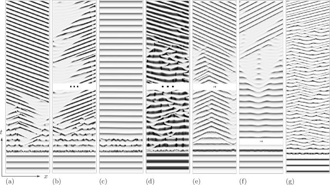
Figure 1: Different regimes resulting from random perturbaton of uniform oscillations. Shown are density plots: space $x$ is horizontal, time $t$ is vertical increasing upwards, $u=1$ corresponds to black and $u=0$ corresponds to white. (a) TB model, $L=15$, taxis ($h_{-}=1$, $h_{+}=0$, $D_{u}=D_{v}=0$), periodic boundary conditions, $t\in[0,2500]$. (b) Same, no-flux boundary conditions, $t\in[0,1200]\cup[43800,45000]$. (c) Same as (a) except $D_{u}=D_{v}=0.05$, $h_{+}=h_{-}=0$. (d) Same as (a) except $w=0.07$, $L=10$, $t\in[0,1200]\cup[36300,37500]$. (e) Same as (a) except $h_{+}=0.1$, $L=50$, $t\in[0,1200]\cup[5000,6200]$. (f) Same as (a) except $h_{+}=0.1$, $D_{u}=D_{v}=0.02$, $L=50$, $t\in[0,400]\cup[1900,3900]$. (g) RM model, $h_{-}=1$, $h_{+}=D_{u}=D_{v}=0$, $L=25$, $t\in[0,2500]$.

The purpose of this communication is to describe new phenomena we have observed in oscillatory systems with “pursuit-evasion” nonlinear cross-diffusion interaction between the components.

II The models

We consider two predator-prey models with cross-diffusion terms of “pursuit-evasion” mutual taxis,

$$\frac{\partial u}{\partial t} = f(u,v)+D_{u}\frac{\partial^{2}u}{\partial x^{2}}+h_{-}\frac{\partial}{\partial x}\left(u\frac{\partial v}{\partial x}\right),$$

$$\frac{\partial v}{\partial t} = g(u,v)+D_{v}\frac{\partial^{2}v}{\partial x^{2}}-h_{+}\frac{\partial}{\partial x}\left(v\frac{\partial u}{\partial x}\right),$$ (2)

for $(x,t)\in[0,L]\times[0,t_{\max}]$ for two reaction kinetics, the Truscott-Brindley (TB) model Truscott and Brindley (1994)

$$f(u,v) = \beta u(1-u)-vu^{2}/(u^{2}+\nu^{2}),$$

$$g(u,v) = \gamma vu^{2}/(u^{2}+\nu^{2})-wv,$$ (3)

where $\beta=0.43$, $\nu=0.053$, $\gamma=0.1$ and $w=0.055$ unless stated otherwise, and the Rosenzweig-MacArthur (MA) model Rosenzweig and MacArthur (1963); Britton (2003); Sherratt and Smith (2008)

$$f(u,v) = \beta u(1-u)-vu/(u+\nu),$$

$$g(u,v) = \gamma vu/(u+\nu)-wv,$$ (4)

where $\beta=1$, $\nu=0.3$, $\gamma=0.15$ and $w=0.03$ unless stated otherwise. Here $u$ represents prey, $v$ predators, the term with $h_{+}$ describes pursuit of prey by predators and the term with $h_{-}$ describes evasion of predators by prey. The simulation were done on an interval $x\in[0,L]$ with periodic or Neumann boundary conditions for both components, using forward Euler stepping in time, center differences for the diffusion terms and upwind difference for the taxis terms, see Tsyganov et al. (2004) for details and justification. Except where stated otherwise, we used discretization steps $\Delta x=0.1$ and $\Delta t=4\cdot 10^{-4}$.

III Numerical observations

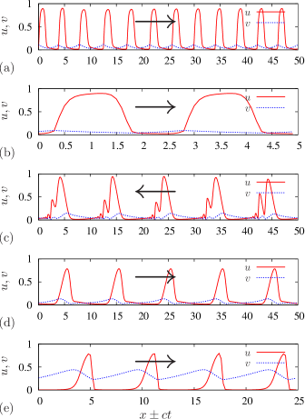
Figure 2: (color online) Examples of profiles of spontaneously established periodic waves. Shown are dependencies of $u$ and $v$ on $x$ at fixed $t$, and direction of propagation by arrows. Parameters are the same as in fig. 1 except interval lentgh $L$, specifically, (a) as in fig. 1(a), (b) as in fig. 1(d), (c) as in fig. 1(e), (d) as in fig. 1(f) and (e) as in fig. 1(g).

Figs. 1 and 2 illustrate the phenomenon of the spontaneous onset of periodic waves. Starting from arbitrary spatially-uniform intial conditions at $t=0$, after a transient allowed to establish uniform oscillations, perturbations were introduced and subsequent evolution observed. The perturbation was introduced at half of the grid points chosen randomly, where at $t=300$ the values of $u$ were replaced by randomly chosen numbers in the interval between $0.15$ and $0.45$. Fig. 1 shows space-time density plots and fig. 2 illustrate selected profiles of the emerging wavetrains.

In the TB model with periodic boundary conditions (fig. 1(a)), after a “random” transient lasting two or three bulk oscillation periods, patterns start to emerge: waves start “from nowhere” and annihilate upon collision with other such waves. After a few periods of such collisions, the waves propagating leftwards win over and a periodic wavetrain establishes which then persists. Different seeds in the random number generator produce solutions differing in details but always leading to periodic trains, leftward and rightward propagating with equal probability (compare density plots and wave profiles in fig. 1 and fig. 2, which corresponded to different simulations with the same parameter sets).

Impenetrable boundaries do not allow periodic wavetrain solutions; however the tendency to establish periodic wavetrains is observed even then. In fig. 1(b) rightward propagating waves win over. Their impact with the right boundary $x=L$ is with partial reflection, when the reflected wave is weak and soon decays; note that this behaviour is typical for collision of solitary excitation waves in such systems Tsyganov et al. (2004). The left boundary has a quenching effect, but at a distance from it waves emerge spontaneously. This distance varies irregularly, indicating that spontaneous generation of waves is associated with an instability, thus sensitive dependence on initial conditions and probably chaotic dynamics. This irregular pattern persists for a long time.

This behaviour is in a contrast with a system with the same kinetics but pure diffusional spatial terms: in fig. 1(c), similar initial random perturbations lead very quickly to re-establishment of spatially uniform oscillations.

The parameters used in fig. 1(a) are close to the boundary of the oscillatory regime in the TB model (achieved e.g. at $w\approx 0.053$ with other parameters fixed). When parameters are further into the oscillatory region, spontaneous generation of periodic wavetrains is still observed, although the transient period of spontaneous wavelet generations and collisions lasts longer, see fig. 1(d).

We have also found that prevalence of the “evasion” taxis ($h_{-}$ coefficient) helps generation of periodic trains, but $h_{+}=0$ is not necessary, and such generation can be observed with the “pursuit” taxis present as well, see fig. 1(e).

Spontaneous generation of periodic trains is observed in the RM model as well, see fig. 1(f).

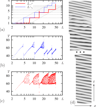
Figure 3: (color online) Variability of the wavetrains at changing $L$. (a) Number of waves in the interval $[0,L]$ as $L$ gradually increases (by $0.2$ every 2000 time units, solid red line) and decreases (by $0.2$ every 1000 time units, dashed blue line). Oblique dashed lines: $n=L/2.5$ and $n=L/8$ to guide the eye. (b) Wave periods measured at a point, as function of $L$ as it decreases. (c) Same, as $L$ increases. (d) Density plots of two episodes of simulation of 1200 time units duration each, with $L$ increasing by $0.2$ every 1000 time units. Lower episode: soft transition from steady 1-wave solution to modulated 1-wave solution ($L:4.8\to 5.6$). Upper episode: subsequent sudden transition from modulated 1-wave solution to a steady 2-wave solution ($L:7.2\to 7.6$).

The spontaneously emerging periodic wavetrains typically had wavelengths in a limited range. To check whether this is dictated by initial conditions or is due to limitations of the system, we performed simulations in a circle, i.e. an interval with periodic boundary conditions, of a slowly changing length $L$. We started from an established propagating wave in a circle. Then we changed the length $L$ of the circle in small steps, allowing sufficient time between the steps for the waves to adjust. During the simulation we monitored the number of waves $n$, determined via the number of points where $u$ crossed the level $u=u_{*}=0.2$, and the periods $T$ defined as intervals between $u$ crossing the level $u=u_{*}$ in the positive direction. Results of one such simulation are shown in fig. 3.

The number of waves $n$ in the interval did not remain constant (fig. 3(a)), but spontaneously adjusted so as to keep the average wavelength within certain limits: between approximately 2.5 and 8 in the simulation shown. This number was not a unique function of the interval length: changing $L$ upwards and downwards produced different dependencies $n(L)$, i.e. we have hysteresis. Simulations at slower rate of change of $L$ slightly changed the $n(L)$ dependencies but the hysteresis stayed. Near the transition points where $n$ changed the value, the propagation of the waves was non-stationary, and was always for $L$ just below the transitional value, whether it was decreasing (fig. 3(b)) or increasing (fig. 3(c)). Increasing $L$ had a noticeably more destabilizing effect than decreasing.

The nature of the non-stationary solutions is illustrated by the density plots shown in fig. 3(d). Starting from an $n=1$ solution, an increase of $L$ above the value of $L\approx 5$ leads to an instability of the steady propagating wave solution. This is a soft, Eckhaus-type instability and leads to a mild modulation of the wave, producing a seemingly two-periodic motion. The amplitude of the modulations grows as $L$ increases, until at $L=7.6$ a qualitative transformation occurs. A gap between the wave and its own copy around the circle grows so big that at a certain moment it is sufficient to allow spontaneous generation of another wave, leading to an $n=2$ solution. This solution is steady, i.e. propagates without modulations, until $L$ grows so big it in turn becomes unstable etc.

IV Preliminary theoretical considerations

Substantial theoretical analysis of the phenomenon of the spontaneous traveling periodic waves is beyond the scope of this communication. Here we consider one naive approach and then some known pattern formation mechanisms, which a priori might look relevant to this phenomenon, only to eliminate them, as not providing a satisfactory explanation. We will refer to the historical review by Cross and Hohenberg (1993, p. 870) (CH for brevity), and to a recent symmetry based classification of instabilities and bifurcations of periodic dissipative waves and structures given by Rademacher and Scheel (2007, p. 2680) (RS for brevity).

It is not captured by lambda-omega approach

The simple class of two-component reaction-diffusion systems introduced by Kopell and Howard (1973) and called “lambda-omega systems”, and closely related to the complex Ginzburg-Landau equation, allows exact solutions in the form of periodic waves. It has offered qualitative insight in many nonlinear wave phenomena, including periodic waves in cyclic populations Sherratt and Smith (2008). However, it does not seem to be helpful in our present case. The modification of the lambda-omega system, corresponding to the choice of signs of taxis terms in (2) is

$$\frac{\partial z}{\partial t}=(\Lambda(|z|)+i\Omega(|z|))z-i\nabla^{2}z$$ (5)

where $z$ is a complex dynamic variable representing $u+iv$, and the purely imaginary diffusivity here corresponds to the absence of self-diffusion, $D_{u}=D_{v}=0$. Then the periodic traveling wave ansatz $z=a\,\exp[i(\omega t-kx)]$, $a,\omega,k\in\mathbb{R}$, gives the finite system

$$\Lambda(a)=0,\qquad\omega=\Omega(a)-k^{2},$$

i.e. all waves have the same amplitude which is a root of $\Lambda()$, and exist for all wavelengths $k$ rather than in a finite interval. Stability analysis and consideration of nonzero self-diffusion do not help either.

It does not emerge via Turing mechanism.

The instability of spatially-uniform solutions in favour of non-oscillatory, spatially-periodic solutions with periods in a finite range is, of course, a defining feature of the Turing patterns, called just so by RS and classified as type $I_{s}$ in CH nomenclature. Cross-diffusion can provide an alternative to the original Turing’s short range inhibition - long range activation condition. Indeed Turing-type instabilities and spontaneously occurring, self-supporting time-stationary spatially periodic patterns have been observed in locally multistable systems with cross-diffusion del Castillo Negrete et al. (2002). Our present observations are different in that here we are dealing with time-oscillating phenomena not just space-oscillating.

It does not emerge via Turing-Hopf mechanism.

A Hopf bifurcation of the spatially uniform equilibrium at a nonzero wavelength, is called “Hopf”, “oscillatory Turing” and “Turing Hopf” instability by RS, classifed as type $I_{o}$ in CH nomenclature, and also known as short-wave instability or finite-wavelength instability. It can lead to stable periodic propagating waves, in lasers, fluid convection and reaction-diffusion models Swift and Hohenberg (1977); Haken (1983); Livshits (1983); Lega et al. (1994). In reaction-diffusion context, such waves have been observed experimentally and in simulations in populations and BZ reaction Mendelson and Lega (1998); Vanag and Epstein (2002). However, the standard way such instability occurs in systems (1) implies existence of an equilibrium that is stable with respect to spatially uniform perturbations, which we do not have here, and it only can occur if $N\geq 3$ whereas we have only two components, $u$ and $v$.

Specifically, for $\mathbf{u}(x,t)=\mathbf{u}_{r}+\mathbf{v}\,e^{\lambda t+ikx}$ where $\mathbf{u}_{r}=(u_{r},v_{r})$ is the spatially uniform equilibrium and $|\mathbf{v}|\ll 1$, we have the characteristic equation

$$\det\left(\mathbf{F}_{r}-\mathbf{D}_{r}k^{2}-\lambda\mathbf{I}\right)=0,$$

where $\mathbf{F}_{r}=\mathbf{F}(\mathbf{u}_{r})=\left(\partial\mathbf{f}/\partial\mathbf{u}\right)_{\mathbf{u}=\mathbf{u}_{r}}=\left[\begin{array}[]{cc}f_{11}&f_{12}\\ f_{21}&f_{22}\end{array}\right]$ is the Jacobian matrix of the reaction terms and $\mathbf{D}_{r}=\mathbf{D}(\mathbf{u}_{r})$ is the diffusion matrix, both evaluated at the equilibrium. Considering for simplicity the cases of fig. 1(a,b,d,f) where $\mathbf{D}_{r}=\left[\begin{array}[]{cc}0&h_{-}u_{r}\\ 0&0\end{array}\right]$, we have

$$\lambda=\frac{1}{2}\left(f_{11}+f_{22}\pm\sqrt{(f_{11}-f_{22})^{2}+4f_{12}f_{21}-f_{21}h_{-}u_{r}k^{2}}\right)$$

which for $k^{2}>\max\left(((f_{11}-f_{22})^{2}+4f_{12}f_{21})/(h_{-}u_{r})\,,\,0\right)$ gives oscillatory behaviour of perturbations, but then $\mathrm{Re}(\lambda)=(f_{11}+f_{22})/2=\mathrm{const}$ whereas it has to have a maximum at a positive $k^{2}$ for this mechanism to be relevant.

It does not emerge via Turing-Hopf instability of spatially uniform oscillations

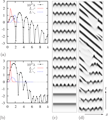
Figure 4: (color online) Emergence of spontaneous periodic waves through instabilities. (a) Spectrum $\lambda(k)$ of harmonic perturbations of the spatially uniform oscillations (black lines with points), and the histograms of the wavenumbers of spontaneous wavetrains in the simulations shown in fig. 3 for increasing $L$ (red solid line) and decreasing $L$ (blue dashed line). (b) Same, for the RM model, parameters as in fig. 1(f), histograms obtained by increasing $L$ by 0.2 every 2000 time units from 5 to 50 and decreasing it back to 2 by 0.2 every 1000 time units. (c) Emergence of standing periodic waves via an instability of the spatially uniform oscillations. Parameters as in fig. 1(a) and fig. 3, $L=12.26$, $\Delta x=L/63$, $\Delta t=5\cdot 10^{-5}$, $t\in[0,1000]$. (d) Emergence of spontaneous periodic wavetrains via an instability of periodic standing waves. Continuation of (c), $t\in[44460,45460]$.

The next possible candidate is the instability of spatially uniform oscillations with respect to perturbations which nonzero freqency and nonzero wavenumber. This case is not considered in the CH nomenclature, and is called “Hopf” instability of spatially homogeneous oscillations, with the same variants as in the previous case, by RS. This instability looks plausible as spatially homogeneous (spatially uniform) oscillations in our systems are indeed possible and even stable in small spatial domains, so we have investigated this possibility with particular care. As limit cycles in the point systems of (3) and (4) can not be described analytically, the investigation of stability has to be done numerically. We have considered solutions of the form $\mathbf{u}(x,t)=\mathbf{u}_{o}(t)+\mathrm{Re}\left(\mathbf{v}(t)e^{ikx}\right)$ with $|\mathbf{v}|\ll 1$, which gives a coupled system of ordinary differential equations

$$\displaystyle{\frac{\mathrm{d}\mathbf{u}_{o}}{\mathrm{d}t}} =\mathbf{f}(\mathbf{u}_{o}),$$ (6a)

$$\displaystyle{\frac{\mathrm{d}\mathbf{v}}{\mathrm{d}t}} =\left(\mathbf{F}(\mathbf{u}_{o})-\mathbf{D}(\mathbf{u}_{o})k^{2}\right)\mathbf{v},$$ (6b)

with parameter $k$. We solved system (6) forward in time with initial conditions for bulk oscillations $\mathbf{u}_{o}$ in the basin of attraction of the limit cycle, and arbitrary nonzero initial conditions for the perturbation $\mathbf{v}$. Then we estimated the Lyapunov exponent for the $\mathbf{v}$-subsystem, $\lambda(k)=\lim_{t\to\infty}t^{-1}\ln(||\mathbf{v}(t)||)$. The estimation was done by finding maxima of the first component of $\mathbf{v}(t)$ and linearly fitting their logarithms against $t$, for an interval of large enough values of $t$. For selected values of $k$ we used two linear independent sets of initial conditions for $\mathbf{v}$, to eliminate the theoretical possibility of accidentally chosing initial conditions that did not lead to the maximal exponent.

The resulting graph $\lambda(k)$ for the TB model at the same parameters as in fig. 1(a) and 3 is shown on fig. 4(a). For comparison, we also show histograms of the empirical wavenumbers observed in simulations shown in fig. 3, calculated as $k=2\pi n/L$, separately for the growing and decreasing $L$. Fig. 4(b) shows similar graphs made for the RM model at the same parameters as in fig. 1(f). It is clear that, although there are finite bands of wavenumbers producing growing perturbations, the actually selected wavenumbers are not the same as those of the fastest growing perturbations, and for the TB model they even partly fall in the interval of decaying perturbations.

Moreover, the growing perturbations of the spatially uniform oscillations in fact do not represent propagating periodic waves, but standing waves. This is illustrated in fig. 4(c) where we show a density plot of a simulation of the full model, similar to fig. 1(a) but with different initial conditions. Here we chose initial conditions as spatially uniform oscillations plus a very small perturbation sinusoidal in space. Note that for the limit of infinitely small perturbation amplitudes this exactly corresponds to system (6).

We conclude that although the cross-diffusion driven instability does indeed take place in the considered examples, the waves that emerge are in fact quite different from the spontaneous periodic traveling waves.

Spontaneous sources as a precursor of spontaneous periodic waves

The periodic standing waves emerging via the cross-diffusion driven instability described above, are in turn unstable themselves. Fig. 4(d) shows a continuation of simulation of fig. 4(c). The standing waves are observed for a long time, as they are stable within the space of functions with spatial period $2\pi/k=L/6$, and the numerical initial conditions are almost exactly periodic with that period, up to small errors resulting from finite precision arithmetics. The small symmetry-breaking numerical errors allow for an instability of the periodic standing waves to develop, during which some of the standing waves occur later than others. When this instability sufficiently develops, there is a sudden, “hard” transition to propagating waves. The spatial period of the propagating waves is twice longer than the spatial period of preceding standing waves. We stress that the traveling waves do not appear via anything like “bifurcation” from standing waves, at least in the examples we considered.

Notice that the long transient solution shown in fig. 4(c,d) is a periodic standing wave by its symmetry, but it also looks like a periodic set of focal sources, synchronously sending out solitary waves which then annihilate each other. As can be seen in fig. 1, apart from the symmetry, this sort of transient before the onset of periodic waves is typical, and only its duration varies in different simulations. That is, the special initial conditions in fig. 4(c,d) only affect the symmetry and the duration of the transient, but not its qualitative character. A similar route to traveling waves via unstable periodic set of “focal sources” standing waves is obseved in the RM model.

V Conclusion

The considered examples demonstrate an unusual type of behaviour. The systems are oscillatory, but the spatially uniform oscillations are unstable. The systems can also demonstrate standing periodic waves, which are also unstable. These instabilities lead to periodic propagating waves, which seems to be the only stable regime. This regime emerges spontaneously even when boundary conditions disallow propagating waves. The periods of the waves can be in a certain interval with strict boundaries, both upper and lower. Nearer the upper end of the interval, i.e. at longer wavelengths, the periodic waves do not propagate steadily but are modulated. Transition from steady to modulated propagation is soft and has empirical features of a supercritical Hopf bifurcation (of a relative equilibrium), i.e. possibly an Eckhaus mechanism.

The defining features described above are sufficiently generic, and the phenomenon of spontaneous periodic traveling waves does not disappear as the parameters are varied, nor it is restricted just to one model. This behaviour does not fall into existing classification of pattern formation scenarios. The detailed mechanisms of spontaneous generation and maintenance of periodic traveling waves require further investigation. However, it is clear that cross-diffusion is an essential factor, since its replacement with, or adding of significant amount of, self diffusion eliminates the effect. Cross-diffusion phenomena are known in a in a variety of physical situations. For example, spontaneous periodic waves have been observed in a Burridge-Knopoff mathematical model of earthquakes Cartwright et al. (1997, 1999). That model belongs to the class (1), with only one nonzero element of matrix $\mathbf{D}$, as in our simulations shown in fig. 1(a) and (g) but constant, and excitable FitzHugh-Nagumo local kinetics. It is not known whether the spontaneous waves in the Burridge-Knopoff model have a finite interval of allowed wavenumbers, as illustrated by fig. 3 for our case, however other described features of those waves are similar to those described here and are likely to have a similar nature. Further investigation of the mechanism of generation of such waves is a subject for further study which is of broad physical interest as a new pattern forming mechanism in dissipative spatially distributed systems.

Returning to the application that originally motivated this study, attempts to explain waves observed in cyclic biological populations, using reaction-diffusion models, had to involve spatially-nonuniform external factors, e.g. sites of increased mortality due to environmental conditions Sherratt et al. (2002); Sherratt and Smith (2008). Such factors are needed to disallow uniform oscillations. Our present results imply that such factors may not be necessary if cross-diffusion interaction are taken into account as the uniform oscillations may be unstable and waves form spontaneously.

Acknowledgments We are grateful to O. Piro for helpful advice. The study was supported in part by RFBR grant 07-04-00363 (Russia) and by a grant from the Research Centre for Mathematics and Modelling of Liverpool University (UK).

References

- Cross and Hohenberg (1993) M. C. Cross and P. C. Hohenberg, Rev. Mod. Phys. 65, 851 (1993).
- Tsyganov et al. (2003) M. A. Tsyganov, J. Brindley, A. V. Holden, and V. N. Biktashev, Phys. Rev. Lett. 91, 218102 (2003).
- Tsyganov et al. (2004) M. A. Tsyganov, J. Brindley, A. V. Holden, and V. N. Biktashev, Physica D 197, 18 (2004).
- Biktashev et al. (2004) V. N. Biktashev, J. Brindley, A. V. Holden, and M. A. Tsyganov, Chaos 14, 988 (2004).
- Tsyganov and Biktashev (2004) M. A. Tsyganov and V. N. Biktashev, Phys. Rev. E 70, 031901 (2004).
- Biktashev and Tsyganov (2005) V. N. Biktashev and M. A. Tsyganov, Proc. Roy. Soc. Lond. A 461, 3711 (2005).
- Tsyganov et al. (2007) M. A. Tsyganov, V. N. Biktashev, J. Brindley, A. V. Holden, and G. R. Ivanitsky, Physics-Uspekhi 50, 275 (2007).
- Vanag and Epstein (2009) V. K. Vanag and I. R. Epstein, Phys. Chem. Chem. Phys. 11, 897 (2009).
- del Castillo Negrete et al. (2002) D. del Castillo Negrete, B. A. Carreras, and V. Lynch, Physica D 168–169, 45 (2002).
- Chung and Peacock-López (2007) J. M. Chung and E. Peacock-López, Phys. Lett. A 371, 41 (2007).
- Truscott and Brindley (1994) J. E. Truscott and J. Brindley, Phil. Trans. Roy. Soc. Lond. ser. A 347, 703 (1994).
- Murray (2002) J. D. Murray, Mathematical Biology I: An Introduction (Springer, New York, NY, 2002).
- Britton (2003) N. F. Britton, Essential mathematical biology (Springer, New York, NY, 2003).
- Sherratt and Smith (2008) J. A. Sherratt and M. J. Smith, Journal of the Royal Society Interface 5, 483 (2008).
- Rosenzweig and MacArthur (1963) M. L. Rosenzweig and R. H. MacArthur, American Naturalist 97, 209 (1963).
- Rademacher and Scheel (2007) J. D. N. Rademacher and A. Scheel, Int. J. of Bifurcation and Chaos 17, 2679 (2007).
- Kopell and Howard (1973) N. Kopell and L. Howard, Stud. Appl. Math. 52, 291 (1973).
- Swift and Hohenberg (1977) J. Swift and P. C. Hohenberg, Phys. Rev. A 15, 319 (1977).
- Haken (1983) H. Haken, Synergetics (Springer, Berlin, Heidelberg, New York, Tokyo, 1983).
- Livshits (1983) M. A. Livshits, Z. Phys. B 53, 83 (1983).
- Lega et al. (1994) J. Lega, J. V. Moloney, and A. C. Newell, Phys. Rev. Lett. 73, 2978 (1994).
- Mendelson and Lega (1998) N. H. Mendelson and J. Lega, Journal of Bacteriology 180, 3285 (1998).
- Vanag and Epstein (2002) V. K. Vanag and I. R. Epstein, Phys. Rev. Lett. 88, 088303 (2002).
- Cartwright et al. (1997) J. H. E. Cartwright, E. Hernandez-Garcia, and O. Piro, Phys. Rev. Lett. 79, 527 (1997).
- Cartwright et al. (1999) J. H. E. Cartwright, V. M. Eguiliz, E. Hernandez-Garcia, and O. Piro, Int. J. of Bifurcation and Chaos 9, 2197 (1999).
- Sherratt et al. (2002) J. A. Sherratt, X. Lambin, C. J. Thomas, and T. N. Sherratt, Proc. Roy. Soc. Lond. ser. B 269, 327 (2002).