Dissipative dynamics of a two - level system resonantly coupled to a harmonic mode

Abstract

We propose an approximation scheme to describe the dynamics of the spin-boson model when the spectral density of the environment shows a peak at a characteristic frequency $\Omega$ which can be very close (or even equal) to the spin Zeeman frequency $\Delta$. Mapping the problem onto a two-state system (TSS) coupled to a harmonic oscillator (HO) with frequency $\omega_{0}$ we show that the representation of displaced HO states provides an appropriate basis to truncate the Hilbert space of the TSS-HO system and therefore a better picture of the system dynamics. We derive an effective Hamiltonian for the TSS-HO system, and show it furnishes a very good approximation for the system dynamics even when its two subsystems are moderately coupled. Finally, assuming the regime of weak HO-bath coupling and low temperatures, we are able to analytically evaluate the dissipative TSS dynamics.

1 Introduction

As new experimental physics techniques allow us to reach minute length scales, and milestones in control and precision of the performed experiments are achieved, the study of open quantum systems has become one of the most prominent areas of modern physics. Moreover, both fundamental and practical aspects of the systems under current investigation help to foment a very broad interest in the area. On the fundamental side, the possibility of having a better comprehension of how classical physics emerges from a quantum system or the realization of very peculiar quantum mechanical states have attracted the interest of many researchers towards the area. From the practical point of view, understanding the main mechanisms leading to the loss of quantum coherence in such systems constitutes a key feature, and one of the major challenges for the physical implementation of, for example, a quantum computer.

A very successful open quantum system which has been investigated to date is a two-state system (TSS) coupled to a dissipative environment. Despite its simplicity, the TSS dissipative dynamics is the paradigm of a wide variety of physical systems. Superconducting devices containing Josephson junctions [1], few-electron semiconductor quantum dots [2] and two-level atoms in optical cavities [3] are just few examples of systems whose low-energy level dynamics can be, in general, captured by a dissipative TSS.

The most studied model of a dissipative TSS is the well-known spin-boson model [4], where the TSS is linearly coupled to the coordinates of a bath of non-interacting oscillators. The dissipative effects of the TSS phenomenological environment are determined by the spectral density of the bath of oscillators [5], which, in general, is assumed to have a power-law behavior at low frequencies. Since it seems that no general analytical solution can be obtained for such a model, several approaches have been proposed to determine the time evolution of the dissipative TSS . Those approaches basically belong to two distinct approximation schemes: one considers a weak TSS-bath coupling in the low-temperature regime, and the other consists in performing an expansion in the tunnelling amplitude $\Delta$ of the TSS states. The first approach is commonly implemented by either using path-integral methods [6] or the Born-Markov approximation (also known as Bloch-Redfield formalism) [7, 8, 9], where only the lowest order terms in the TSS-bath coupling are taken into account for the TSS dissipative dynamics. The other scheme has been shown to be a fair approximation specially in the regimes of strong damping and/or high temperatures, and also employs path-integral methods within the so-called noninteracting blip approximation (NIBA) as its main technique [4, 6].

An emerging problem in the area of dissipative TSSs is the one in which the bath effective spectral density $J_{eff}(\omega)$ presents a pronounced peak (resonance) at a characteristic frequency $\Omega$. A typical example of such a case happens when the energy scale of the device used to detect the state of the TSS is comparable to that of its own regime of operation. Since the device, or “quantum detector”, also suffers from the dissipative effects of the environment, the TSS-detector resonance constitutes an efficient channel for decoherence processes to take place. For example, as the energy scale of superconducting qubits reaches the order of several GHz, this mechanism shows up on these systems due to their coupling to the read-out dc-SQUIDs [10, 11]. In addition to the TSS-detector case, the presence of a structured bath with a sharp peak has also been discussed in other pertinent contexts, e. g., electron transfer in biological and chemical systems [12] and semiconductor quantum dots [13], to name just a few relevant problems of this growing interest subject.

Indeed, it has been shown [14, 15, 11] that the structure of the environment becomes an essential feature of the dissipative TSS dynamics when its frequency is comparable to the bath resonance frequency $\Omega$. Not only the decay rates cannot be correctly determined by a perturbative approach in the TSS-bath coupling, but such an approximation also fails to account for the presence of additional resonances in the TSS dynamics. By using an exact mapping [12] of the spin-boson problem with a structured environment onto that of a TSS coupled to a single HO system with frequency $\Omega$, which itself interacts with a bath of oscillators having an Ohmic spectral density, several techniques have been applied to the investigation of the TSS dissipative dynamics. When the single HO is strongly damped and/or coupled to a bath at high temperatures, the NIBA has been employed to both TSS-HO weak [11] and strong [16] coupling cases. On the other hand, the numerically exact method of the quasi-adiabatic propagator path-integral (QUAPI) [14, 11], as well as a three-level system (3LS) Redfield theory, have indicated the failure of the perturbative approaches in the HO-bath weak coupling and low temperatures regimes.

In this work, we present an approximation scheme to describe the dynamics of the spin-boson problem with a structured bath having a pronounced resonance at frequency $\Omega$. Following previous works [12, 14, 13], we map this problem onto a TSS coupled to a single HO with frequency $\omega_{0}$. In order to obtain an appropriate effective Hamiltonian for the lowest-lying energy states of the TSS-HO system, we show that the representation of displaced HO states whose displacement depends on the TSS state, provides a better picture of the system dynamics, and consequently the appropriate basis to truncate the Hilbert space of the TSS-HO system. We show that the derived effective Hamiltonian furnishes a very good approximation for a vast range of the physical parameters of the system even when the TSS and the HO are moderately coupled close to the resonance. In addition, assuming the regime of weak HO-bath coupling and low temperatures, we are able to analytically evaluate the dissipative TSS spin dynamics.

This paper is organized as follows. In section 2 we present the model for the system, and derive the effective Hamiltonian using the approximation scheme proposed above. By varying the physical parameters of the problem, we compare its predictions with: (1) an exact numerical calculation (for which we found to be sufficient to consider a $N=18$ dimensional TSS-HO Hilbert space); and (2) the simple truncation of the TSS-HO Hilbert space. Section 3 contains the results obtained for the TSS-HO dissipative dynamics assuming the regime of HO-bath weak-coupling and low-temperatures. Finally, in section 4, we present our concluding remarks.

2 The model

Our starting point for describing the TSS dissipative dynamics in the presence of a structured environment is the spin-boson Hamiltonian [4],

$$\hat{H}_{SB}=-\frac{\hbar}{2}\Delta\hat{\sigma}_{x}+\sum_{k}\hbar\omega_{k}\hat{b}^{\dagger}_{k}\hat{b}_{k}+\hbar\hat{\sigma}_{z}\sum_{k}c_{k}(\hat{b}^{\dagger}_{k}+\hat{b}_{k}),$$ (1)

where $\hat{\sigma}_{i}$ are the Pauli matrices and $\hbar\Delta$ represents the tunnelling amplitude between the TSS states.

The bath of oscillators, introduced by the canonical bosonic creation and annihilation operators $\hat{b}_{k}^{\dagger}$ and $\hat{b}_{k}$, is assumed to have a spectral density $J_{eff}(\omega)$ showing a Lorentzian peak at a characteristic frequency $\Omega$.

It has been shown [12, 13] that the proposed problem can be mapped onto a system comprised of a TSS coupled to a single HO of frequency $\omega_{0}$, which itself interacts with a bath of oscillators having a spectral density $J(\omega)$ presenting a power-law frequency distribution. The system Hamiltonian in this formulation is given by

$$\hat{H}=-\frac{\hbar}{2}\Delta\hat{\sigma}_{x}+\hbar\omega_{0}\hat{a}^{\dagger}\hat{a}+\hbar\hat{\sigma}_{z}(g\hat{a}^{\dagger}+g^{\ast}\hat{a}){}$$ (2)

$$\qquad\qquad+\sum_{k}\hbar\omega_{k}\hat{b}^{\dagger}_{k}\hat{b}_{k}+\hbar(\hat{a}^{\dagger}+\hat{a})\sum_{k}\lambda_{k}(\hat{b}^{\dagger}_{k}+\hat{b}_{k}),$$

where $\hat{a}^{\dagger}$ and $\hat{a}$ are the creation and annihilation operators of the single HO system, and $g$ stands for the TSS-HO coupling constant. If $g$ is a real function, the TSS-HO coupling has the form of a $``\hat{\sigma}_{z}$-coordinate” interaction. On the other hand, if $g$ is a purely imaginary function, the TSS-HO coupling becomes a $``\hat{\sigma}_{z}$-momentum” interaction.

From the system Hamiltonian (2), one can observe that the dissipative effects of the environment on the TSS dynamics occur only indirectly through the TSS-HO interaction. Thus, in this formulation, it is clear that the TSS-HO coupling works as a dissipative channel for the TSS. Such a channel can be enhanced or suppressed depending on how strongly coupled the TSS and HO systems are. This depends not only on the strength of the coupling constant $g$, but also on how far from resonance these two subsystems are. Indeed, if we assume a $``\hat{\sigma}_{z}$-coordinate” coupling, i. e., $g=g^{\ast}$, and an Ohmic spectral density $J(\omega)$,

$$J(\omega)=\frac{\pi}{2}\sum_{k}\lambda^{2}_{k}\delta(\omega-\omega_{k})=\kappa\omega e^{-\omega/\omega_{c}},$$ (3)

one can show [12] that the corresponding exact mapping between the Hamiltonians in (1) and (2) occurs when the single HO has its frequency given by the $J_{eff}(\omega)$ resonance frequency $\Omega$, i. e., $\omega_{0}=\Omega$. Consequently, the peak in the effective spectral density of the bath “seen” by the TSS, $J_{eff}(\omega)$, can be interpreted as a manifestation of a definite resonance of one of the environment degrees of freedom.

Recently, Westfahl Jr. and collaborators [13] have demonstrated that a “$\hat{\sigma}_{z}$-momentum” TSS-HO coupling, i. e., $g=-g^{\ast}$, with a power-law frequency dependence for $J(\omega)$ ($J(\omega)\propto\omega^{s}$), leads to a significant change of the effective bath spectral density $J_{eff}(\omega)$ of the system Hamiltonian (1). Although $J_{eff}(\omega)$ still shows a pronounced peak, featuring an approximated Lorentzian shape, its characteristic frequency $\Omega$ does not match the single HO frequency $\omega_{0}$, i. e. $\Omega\neq\omega_{0}$. Indeed, investigating the dissipative effects, due to the spin-orbit mechanism, on the electronic spin dynamics trapped in quantum dots, they have found that the characteristic resonance frequency $\Omega$ predicted for the effective bath spectral density $J_{eff}(\omega)$ is, in general, shifted to a value much lower than that of the single HO, $\Omega\ll\omega_{0}$. In addition, they have shown that such a resonance occurs in a frequency regime which can be, in principle, of the order of the Zeeman frequency of the spin, raising concerns about the appropriate approach to correctly describe the dissipative spin dynamics.

Thus, since the system Hamiltonian (2) is capable of describing the dissipative dynamics of a TSS coupled to a variety of structured environments, from here onwards, we shall focus on describing its features and properties. Unfortunately, despite its simplicity, the Hamiltonian (2) cannot be analytically diagonalized. However, since our final goal is to determine the TSS dissipative dynamics in the regime of low temperatures, $\hbar\Delta\gg k_{B}T$, we can concentrate on determining its low-energy level spectrum. In addition, we are going to assume that the HO dynamics is subject to weak dissipation, in such a way that its states are weakly perturbed by the HO-bath coupling.

Under these considerations, in order to find a low-dimensional effective Hamiltonian for the TSS-HO system, the natural procedure is to perform a truncation of the HO Hilbert space, thus reducing the TSS-HO Hilbert space dimensionality. The simplest method of doing that consists in considering only the ground, $|0\rangle$, and first excited, $|1\rangle$, states of the HO, leading to a four-dimensional Hilbert space of the composite TSS-HO system.

However, as depicted in Fig. 1, that approximation fails as soon as the condition of a TSS-HO weak coupling, $g\ll\Delta,\omega_{0}$ , is not satisfied. Comparing with a numerical calculation performed by taking into account a $N=18$ dimensional Hilbert space, we can see the system Bohr frequencies $\omega_{01}$ and $\omega_{02}$ such that $\hbar\omega_{01}\equiv E_{1}-E_{0}$ and $\hbar\omega_{02}\equiv E_{2}-E_{0}$, where $E_{0},E_{1}$ and $E_{2}$ respectively correspond to the eingenenergy of the ground, first and second excited states, can deviate circa $10\%$ from the correct values, even for moderate TSS-HO couplings. Since we expect a sharp resonance for the effective spectral density $J_{eff}(\omega)$, those deviations can easily lead to much larger errors when computing the TSS relaxation rates. Indeed, Thorwart and collaborators [14] report deviations for the relaxation rates of the order of $\approx 20\%$ for the weak coupling case $g=0.07$, when performing the simple truncation of the HO Hilbert space.

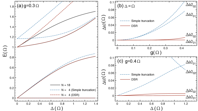
Figure 1: (a) The four lowest levels of the TSS-HO system, as a function of the tunnelling frequency $\Delta$, for the moderate coupling case $g=0.3\Omega$, obtained through: numerical calculation considering a $N=18$ dimensional Hilbert space (black solid curve); analytical solution after performing a simple truncation of the HO Hilbert space (blue dot-dashed curve); and analytical solution of the effective Hamiltonian derived, Eq. (8), in the HO displaced state representation (DSR) (red dashed curve). (The ground state is taken having $E=0$). (b) and (c) present the $\omega_{01}$ and $\omega_{02}$ frequency deviations, $\Delta\omega_{0i}=\omega_{0i}^{ST,DSR}-\omega_{0i}^{(N=18)}$, for the simple truncation approximation and the effective Hamiltonian Eq. (8), as a function of the TSS-HO coupling $g$ (for the resonance case $\Delta=\Omega$), and the tunneling amplitude $\Delta$ (assuming $g=0.4\Omega$).

The failure of the simple truncation of the HO Hilbert space for cases other than the TSS-HO weak coupling, $g\ll\Delta,\Omega$ , was already expected, since it does not correctly take into account the weight of the higher energy HO states in the spectral decomposition of the lowest energy eigenstates of the Hamiltoninan (2). As one can observe from the latter equation, the TSS-HO interaction term has the net effect of inducing displacements of the HO in its phase space $\{q,p\}$, hence leading to the mixing of the HO eigenstates of Eq.(2). So, the stronger the TSS-HO coupling is, the more important the HO higher energy states become.

Therefore, in order to obtain a better picture of the lowest energy states of Eq. (2), we have to perform the truncation of the HO Hilbert space in a representation where such an effect is taken into account. In other words, it is the displaced harmonic oscillator states which ought to be the appropriate basis where one should perform the reduction of Hilbert space of the TSS-HO system.

The change of representation can be done by introducing the unitary HO displacement operator $\hat{D}(\alpha)=e^{\alpha\hat{a}^{\dagger}-\alpha^{\ast}\hat{a}}$, which is very well-known in the context of coherent states [3]. There, among several other implications, the parameter $\alpha$ is a $c$-number, such that the transformation $\hat{D}^{\dagger}(\alpha)\hat{a}\hat{D}(\alpha)=\hat{a}+\alpha$ has the action of shifting the HO canonical position and momentum operators by amounts proportional to, ${\rm Re}(\alpha)$ and ${\rm Im}(\alpha)$, respectively. However, an important feature of the Hamiltonian (2) is the fact that the displacements of the HO states depend on the state of the TSS. Therefore, we are led to introduce the unitary transformation

$$\hat{D}(s,\hat{\sigma}_{z})\equiv e^{(s\hat{a}^{\dagger}-s^{\ast}\hat{a})\hat{\sigma}_{z}},$$ (4)

as the conditional displacement operator of Eq.(2). Here, we consider the displacement parameter $s$ as an ad hoc parameter of our model, to be properly chosen in order to obtain the best effective Hamiltonian possible.

Transformation (4) is very similar to what is known in the literature as the polaron transformation [4, 6]. Indeed, if we had followed, by analogy, the choice made for the polaron transformation, we would have obtained $s=-g/\omega_{0}$. Although it correctly diagonalizes the Hamiltonian (2) when $\Delta=0$, this choice is expected to fail, as discussed in [17], when the tunnelling amplitude becomes appreciable, since from its analytical solution one obtains $\omega_{01}\rightarrow\infty$, instead of $\omega_{01}\rightarrow\omega_{0}$, when $\Delta\rightarrow\infty$.

Thus, in order to make the best choice for the ad hoc parameter $s$, we have to carefully observe which one would reflect the kind of dynamics we should expect for our TSS-HO system. Performing the change of representation, $\tilde{H}\equiv\hat{D}^{\dagger}\hat{H}\hat{D}$, and truncating the HO Hilbert space, one finds

$$\tilde{H}_{TSS-HO}=-\frac{\hbar}{2}\tilde{\Delta}\hat{\sigma}_{x}\left(1-4|s|^{2}\hat{c}^{\dagger}\hat{c}\right)+\hbar\omega_{0}\hat{c}^{\dagger}\hat{c}$$

$$\qquad+\hbar\hat{c}^{\dagger}\left\{\hat{\sigma}_{z}(g+\omega_{0}s)+i\hat{\sigma}_{y}s\tilde{\Delta}\right\}+\hbar\hat{c}\left\{\hat{\sigma}_{z}(g^{\ast}+\omega_{0}s^{\ast})-i\hat{\sigma}_{y}s^{\ast}\tilde{\Delta}\right\},$$ (5)

where, in order to stress the fact that we are now working with a reduced Hilbert space, we have defined the operators $\hat{c}\equiv|\tilde{0}\rangle\langle\tilde{1}|$ and $\hat{c}^{\dagger}\equiv|\tilde{1}\rangle\langle\tilde{0}|$, in which $|\tilde{0}\rangle$ and $|\tilde{1}\rangle$ represent, respectively, the ground and first excited states of the displaced HO. $\tilde{\Delta}$ represents the renormalized tunnelling amplitude due to the TSS-HO coupling, which is given by

$$\tilde{\Delta}\equiv\Delta e^{-2|s|^{2}}.$$ (6)

Without dissipation, the TSS-HO system should evolve in time in such a way there would be a persistent exchange of a quantum of energy between the two subsystems. Such a dynamical behaviour has a precise analogue in the problem of absorption (emission) of a single photon by (from) an atom placed in an optical cavity. There, the fundamental tool for the study of the system dynamics is the so-called Jaynes-Cummings (JC) Hamiltonian. Inspecting Eq. (5), one can see that the choice

$$s\equiv-\frac{g}{\omega_{0}+|\tilde{\Delta}|},$$ (7)

leads us to the same form as a JC Hamiltonian. It worth noting that one could use a variational calculation to determine the value of the parameter $s$ for the polaron transformation Eq. (4). Indeed, by minimizing the free energy of the system using the Bogoliubov-Peierls bound, Silbey and Harris [18] could determine a transcendental equation for $s$. For the unbiased case and $T=0$, that leads to a very similar renormalized tunnelling amplitude to that found in Eq. (6) (cf. Eq. (103) in the review [19])

Assuming $\Delta\leq 0$, the effective Hamiltonian in the HO displaced state representation (DSR) obtained using Eq.(7) in Eq.(5) reads

$$\tilde{H}_{DSR}\equiv-\frac{\hbar}{2}\tilde{\Delta}\hat{\sigma}_{x}\left(1-\frac{4|g|^{2}}{(\omega_{0}+|\tilde{\Delta}|)^{2}}\hat{c}^{\dagger}\hat{c}\right)+\hbar\omega_{0}\hat{c}^{\dagger}\hat{c}$$

$$\qquad+\frac{2\hbar|\tilde{\Delta}|}{\omega_{0}+|\tilde{\Delta}|}(g\hat{c}^{\dagger}\hat{\sigma}^{(x)}_{-}+g^{\ast}\hat{c}~{}\hat{\sigma}^{(x)}_{+}),$$ (8)

where we have introduced the ladder operators for the spin $x-$component, $\hat{\sigma}_{\pm}^{(x)}=\frac{1}{2}(\hat{\sigma}_{z}\mp i\hat{\sigma}_{y})$. The Hamiltonian (8) can be diagonalized analytically, yielding eigenenergies given by

$$E_{0}\equiv-\frac{\hbar}{2}\tilde{|\Delta|},\qquad E_{3}\equiv\frac{\hbar}{2}|\tilde{\Delta}|\left\{1-\frac{4|g|^{2}}{(\omega_{0}+|\tilde{\Delta}|)^{2}}\right\}+\hbar\omega_{0},~{}{\rm and}$$ (9)

$$E_{1,2}\equiv\frac{\hbar}{2}\left\{2\omega_{0}-\frac{E_{3}+E_{0}}{\hbar}\mp\sqrt{\left(\frac{E_{3}-E_{0}}{\hbar}-2\omega_{0}\right)^{2}+\frac{16|g|^{2}\tilde{\Delta}^{2}}{(\omega_{0}+|\tilde{\Delta}|)^{2}}}\right\}.$$ (10)

The analysis of the obtained eigenenergies $E_{i}$, Eqs. (9) and (10), reveals that the Hamiltonian (8) provides the correct results for certain limits of the parameters of Eq. (2), namely: (1) as $\omega_{0}\rightarrow\infty$, we obtain $\omega_{01}\rightarrow|\Delta|$; (2) for $|\Delta|\rightarrow\infty$, we have $\omega_{01}\rightarrow\omega_{0}$; and for the resonant case $\Delta=\omega_{0}$, with $g\ll\Delta,\omega_{0}$, we find $\omega_{01}\approx\omega_{0}-g$ and $\omega_{02}\approx\omega_{0}+g$. Moreover, as one can see from Fig. 1, the resulting Hamiltonian (8) gives a very good approximation of our problem for a vast range of the physical parameters $\Delta$ and $g$. In fact, the largest deviations we have found considering the parameters illustrated in Fig. 1 were $\Delta\omega_{01}\approx 0.07\%$ and $\Delta\omega_{02}\approx 0.6\%$. It is worth noting that, when performing the simple truncation, this level of agreement can only be met for the ground and first excited states if we consider a $N=8$ dimensional Hilbert space. Indeed, for a $N=6$ dimensional Hilbert space we found: $\Delta\omega_{01}^{(N=6)}\approx 20\Delta\omega_{01}^{DSR}$ and $\Delta\omega_{02}^{(N=6)}\approx 3\Delta\omega_{02}^{DSR}$, while for the case $N=8$ we obtained: $\Delta\omega_{01}^{(N=8)}\approx 1.3\Delta\omega_{01}^{DSR}$ and $\Delta\omega_{02}^{(N=8)}\approx 0.34\Delta\omega_{02}^{DSR}$.

Finally, defining the states $|\pm\rangle$ as the eigenstates of $\hat{\sigma}_{x}$, $\hat{\sigma}_{x}|\pm\rangle=\pm|\pm\rangle$, the eigenstates of the Hamiltonian (8) can be written in the form

$$|e_{0}\rangle\equiv|-,\tilde{0}\rangle,\qquad|e_{3}\rangle\equiv|+,\tilde{1}\rangle,\quad|e_{1}\rangle\equiv A|+,\tilde{0}\rangle+B|-,\tilde{1}\rangle,~{}{\rm and}$$ (11)

$$|e_{2}\rangle\equiv-B|+,\tilde{0}\rangle+A|-,\tilde{1}\rangle,$$ (12)

where, $A\equiv(E_{0}+E_{2})/\sqrt{(E_{0}+E_{2})^{2}+4|g|^{2}\tilde{\Delta}^{2}\hbar^{2}/(\omega_{0}+|\tilde{\Delta}|)^{2}}$ and $B^{2}=1-A^{2}$.

The eigenstates $|e_{1,2}\rangle$, Eqs. (11) and (12), reveal the hybridization process occurring between the TSS and HO states due to their coupling. Indeed, if $g=0$, i. e., the case of a decoupled TSS-HO system, the eigenstates of Eq. (8) are simple tensor product of the TSS and HO eigenstates ($A=1$). Nevertheless, as one increases the coupling $g$, the system eigenstates become more hybridized. At the resonance condition, $\omega_{0}=\Delta$, the eigenstates $|e_{1,2}\rangle$ become nearly the maximally entangled TSS-HO states, with $A\approx\frac{1}{\sqrt{2}}(1+O(g))$.

3 Dissipative dynamics

The evaluation of the dissipative TSS dynamics can be described, for a weak HO-bath coupling and low temperatures, using the Redfield equations [6]

$$\dot{\tilde{\rho}}_{nm}(t)=-i\omega_{nm}\tilde{\rho}_{nm}(t)-\sum_{k,l}R_{nmkl}\tilde{\rho}_{kl}(t),$$ (13)

where the matrix elements $\tilde{\rho}_{nm}\equiv\langle n|\tilde{\rho}|m\rangle$ are taken using the eigenstates of Eq. (8), and the Redfield tensors are given by $R_{nmkl}=\delta_{lm}\sum_{r}\Gamma_{nrrk}^{(+)}+\delta_{nk}\sum_{r}\Gamma_{lrrm}^{(-)}-\Gamma_{lmnk}^{(+)}-\Gamma_{lmnk}^{(-)}$, with

$$\Gamma_{lmnk}^{(+)}=\hbar^{-2}\int_{0}^{\infty}dte^{-i\omega_{nk}t}\langle\tilde{\cal{H}}_{I,lm}(t)\tilde{\cal{H}}_{I,nk}(0)\rangle,$$ (14)

$$\Gamma_{lmnk}^{(-)}=\hbar^{-2}\int_{0}^{\infty}dte^{-i\omega_{lm}t}\langle\tilde{\cal{H}}_{I,lm}(0)\tilde{\cal{H}}_{I,nk}(t)\rangle,$$ (15)

where $\tilde{\cal{H}}_{I}(t)=e^{i\tilde{H}_{R}t/\hbar}\tilde{H}_{I}e^{-i\tilde{H}_{R}t/\hbar}$ is the interaction Hamiltonian in the interaction picture, and the brackets represent thermal averages over the bath degrees of freedom. Here, we denote $\tilde{H}_{R}$ and $\tilde{H}_{I}$ as the bath and HO-bath interaction Hamiltonians obtained from Eq. (2) under the transformation presented in the last section. The full Hamiltonian now reads

$$\tilde{H}=\tilde{H}_{DSR}+\sum_{k}\hbar\omega_{k}\hat{b}_{k}^{\dagger}\hat{b}_{k}+\left(\hat{c}^{\dagger}+\hat{c}-\frac{2{\rm Re}(g)}{\omega_{0}+|\tilde{\Delta}|}\hat{\sigma}_{z}\right)\sum_{k}\hbar\lambda_{k}(\hat{b}^{\dagger}+\hat{b}_{k}).$$ (16)

where the second and third terms on the RHS of this equation are, respectively, $\tilde{H}_{R}$ and $\tilde{H}_{I}$. It is worth noting that the term proportional to Re$(g)$ in $\tilde{H}_{I}$, Eq. (16), represents a correction naturally introduced by the scheme proposed, and leads to an effective interaction between the TSS and bath mediated by the TSS-HO coupling. Had we followed the simple truncation approximation, such a term would not be present in the system dynamics. We have seen that this term can represent a non-negligible correction to the system-bath interaction, since it can reach fractions of few percent of the latter, e. g., for $g=0.1,\Delta=\omega_{0}=1$, we find $||2{\rm Re}(g)/(\omega_{0}+|\tilde{\Delta}|)||/||\hat{c}^{\dagger}+\hat{c}||\approx 0.1$.

In order to be able to analyze the resonance case, $\omega_{0}=\Delta$, as pointed out in Ref. [14], we have to go beyond the two-level approximation when using the Redfield equations (13). Indeed, since a two-level approximation is not capable of taking into account the hybridization of TSS-HO states, it fails to present the additional resonances of the TSS dynamics. Thus, considering a three-level system, one can determine the expectation value of $\sigma_{z}$, $\sigma_{z}={\rm Tr}(\hat{\rho}(t)\hat{\sigma}_{z})$, as

$$\sigma_{z}(t)\approx 2{\rm Re}\left(A\langle e_{0}|\tilde{\rho}|e_{1}\rangle-B\langle e_{0}|\tilde{\rho}|e_{2}\rangle\right).$$ (17)

Performing the secular approximation [7], we can neglect the terms $R_{nmkl}$ of $\tilde{\rho}_{nm}$ for which $\omega_{nm}\neq\omega_{kl}$. This leads us to the following set of coupled differential equations

$$\dot{\tilde{\rho}}_{01}\equiv\langle e_{0}|\dot{\tilde{\rho}}|e_{1}\rangle\approx i\omega_{01}\tilde{\rho}_{01}-\gamma_{1}\tilde{\rho}_{01}-\gamma_{2}\tilde{\rho}_{02},$$ (18)

$$\dot{\tilde{\rho}}_{02}\equiv\langle e_{0}|\dot{\tilde{\rho}}|e_{2}\rangle\approx i\omega_{02}\tilde{\rho}_{02}-\gamma_{3}\tilde{\rho}_{01}-\gamma_{4}\tilde{\rho}_{02},$$ (19)

where $\gamma_{1}=R_{0101},\gamma_{2}=R_{0102},\gamma_{3}=R_{0201},~{}{\rm and}~{}\gamma_{4}=R_{0202}$. Assuming that $J(\omega)$ is a regular function in the complex plane, we can analytically evaluate the Redfield rates, obtaining

$${\rm Re}~{}\Gamma_{lmnk}^{(+)}=(\tilde{h}_{lm}\tilde{h}_{mk})J(|\omega_{nk}|)\frac{e^{-\beta\hbar\omega_{nk}/2}}{\sinh(\beta\hbar|\omega_{nk}|/2)}$$ (20)

$${\rm Im}~{}\Gamma_{lmnk}^{(+)}=-\frac{2}{\pi}(\tilde{h}_{lm}\tilde{h}_{mk}){\rm P}\int_{0}^{\infty}d\omega\frac{J(\omega)}{\omega^{2}-\omega_{nk}^{2}}\left(\omega-\omega_{nk}\coth(\frac{\beta\hbar\omega}{2})\right)$$ (21)

where $\tilde{h}_{lm}\equiv\langle l|(\hat{c}^{\dagger}+\hat{c}-\frac{2{\rm Re}(g)}{\omega_{0}+|\tilde{\Delta}|}\hat{\sigma}_{z})|m\rangle$. In addition, using the relation $\Gamma_{knml}^{(-)}=(\Gamma_{lmnk}^{(+)})^{\ast}$, we can determine the Redfield tensors $R_{nmkl}$ in terms of the rates $\Gamma_{lmnk}^{(+)}$.

From Eqs. (17-19), we find the spectral decomposition of $\sigma_{z}$ as

$$\omega_{\pm}=\frac{\omega_{01}+\omega_{02}}{2}+i\left(\frac{\gamma_{1}+\gamma_{4}}{2}\right)\pm\sqrt{\left(\frac{\omega_{01}-\omega_{02}}{2}+\frac{i}{2}(\gamma_{1}-\gamma_{4})\right)^{2}-\gamma_{2}\gamma_{3}}$$ (22)

where Re$(\omega_{\pm})$ are the main oscillation frequencies of the $\sigma_{z}$ dynamics, and Im$(\omega_{\pm})$ gives their respective damping rates.

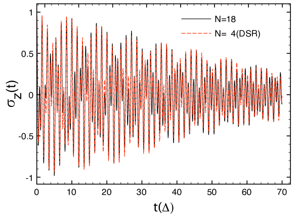
Figure 2: $\sigma_{z}(t)$ dissipative dynamics for the resonant case, $\Delta=\omega_{0}$, computed for an Ohmic spectral density, Eq. (3), with $\kappa=0.02$, $\omega_{c}=10\Delta$ and temperature $k_{B}T=0.1\hbar\Delta$. We assumed a $\sigma_{z}-$coordinate TSS-HO coupling, with constant coupling given by $g=0.3\Delta$. Two main oscillation frequencies $\omega_{\pm}$, Eq. (22), are observed in the dynamics, reflecting the hybridization of the TSS-HO states. Solid and dotted lines represent, respectively, the $N=18$ dimensional Hilbert space and our $N=4$ truncated space in the DSR.

Figure 2 presents a typical time evolution for $\sigma_{z}$ for the resonant case using Eq. (22). Once again, by comparing it to the dynamics presented by a larger Hilbert space, $N=18$, we can verify a very good agreement of the results obtained using the scheme developed in section 2 . As one can observe, the TSS dynamics presents a rich structure, with the presence of two main oscillation frequencies, which are due to the TSS-HO resonance. These results corroborated those obtained in [14, 15, 11].

4 Conclusions

In conclusion, we presented and discussed a new approximation scheme to describe the dynamics of the spin-boson model with a structured environment. We studied the proposed problem by exploring its exact mapping onto that of a TSS coupled to a single HO of frequency $\omega_{0}$, which itself interacts with a bath of oscillators. We showed that, in order to find a low-dimensional effective Hamiltonian for the TSS-HO system, the representation of displaced HO states, DSR, provides an appropriate basis to truncate its Hilbert space. For that, we defined a conditional displacement operator, where the shifting of the HO system was dependent of the state of the TSS. In so doing we needed to introduce an ad hoc displacement parameter $s$ which should be chosen in such a way that the best effective Hamiltonian could be obtained. Invoking the physics of an atom-cavity system, we chose the parameter $s$ such that the effective Hamiltonian had a Jaynes-Cummings form. By comparing our numerical results with those considering a larger Hilbert space, we showed that, in fact, the derived effective Hamiltonian gives an excellent approximation of the original problem for a vast range of its physical parameters even when the TSS and the HO are moderately coupled close to the resonance. Actually, we showed that in order to achieve the same level of precision of the low-dimensional DSR model one needs to, at least, double the dimensionality of Hilbert space of the system within the simple truncation approximation. Finally, assuming the regime of weak HO-bath coupling and low temperatures, we were able to analytically determine the dissipative TSS dynamics using a $3$LS Redfield theory.

5 Acknowledgements

AOC would like to thank the CNPq (Conselho Nacional de Desenvolvimento Científico e Tecnológico) and the Millenium Institute for Quantum Information for financial support.

References

References

- [1] Yuriy Makhlin, Gerd Schön, and Alexander Shnirman. Quantum-state engineering with josephson-junction devices. Rev. Mod. Phys., 73(2):357–400, May 2001.
- [2] R. Hanson, L. P. Kouwenhoven, J. R. Petta, S. Tarucha, and L. M. K. Vandersypen. Spins in few-electron quantum dots. Rev. Mod. Phys., 79(4):1217, 2007.
- [3] C. Tannoudji, C. Dupont-Roc, and J. Grynberg. Atom Photon Interaction: Basic Processes and Applications. Wiley, New York, 1992.
- [4] A. J. Leggett, S. Chakravarty, A. T. Dorsey, Matthew P. A. Fisher, Anupam Garg, and W. Zwerger. Dynamics of the dissipative two-state system. Rev. Mod. Phys., 59(1):1–85, Jan 1987.
- [5] A. O. Caldeira and A. J. Leggett. Quantum tunnelling in a dissipative system. Annals of Physics, 149(2):374–456, Oct 1983.
- [6] U. Weiss. Quantum Dissipative Systems. World Scientific, Singapore, 2nd edition edition, 1999.
- [7] A. G. Redfield. On the theory of relaxation processes. IBM Journal of Research and Development, 1(1):19–31, Jul 1957.
- [8] Ludwig Hartmann, Igor Goychuk, Milena Grifoni, and Peter Hänggi. Driven tunneling dynamics: Bloch-redfield theory versus path-integral approach. Phys. Rev. E, 61(5):R4687–R4690, May 2000.
- [9] David P. DiVincenzo and Daniel Loss. Rigorous Born approximation and beyond for the spin-boson model. Physical Review B (Condensed Matter and Materials Physics), 71(3):035318, 2005.
- [10] I. Chiorescu, Y. Nakamura, C. J. P. M. Harmans, and J. E. Mooij. Coherent Quantum Dynamics of a Superconducting Flux Qubit. Science, 299(5614):1869–1871, 2003.
- [11] M. C. Goorden, M. Thorwart, and M. Grifoni. Entanglement spectroscopy of a driven solid-state qubit and its detector. Phys. Rev. Lett., 93(26):267005, Dec 2004.
- [12] Anupam Garg, Jose Onuchic, and Vinay Ambegaokar. Effect of friction on electron transfer in biomolecules. J. Chem. Phys., 83(9):4491–4503, Nov 1985.
- [13] Harry Westfahl, Amir O. Caldeira, Gilberto Medeiros-Ribeiro, and Maya Cerro. Dissipative dynamics of spins in quantum dots. Phys. Rev. B, 70(19):195320, Nov 2004.
- [14] M. Thorwart, E. Paladino, and M. Grifoni. Dynamics of the spin-boson model with a structured environment. Chem. Phys., 296:333–344, 2004.
- [15] F. K. Wilhelm, S. Kleff, and J. von Delft. The spin-boson model with a structured environment: a comparison of approaches. Chem. Phys., 296:345–353, 2004.
- [16] F Nesi, M Grifoni, and E Paladino. Dynamics of a qubit coupled to a broadened harmonic mode at finite detuning. New Journal of Physics, 9(9):316, 2007.
- [17] Frederico Brito, David P DiVincenzo, Roger H Koch, and Matthias Steffen. Efficient one- and two-qubit pulsed gates for an oscillator-stabilized josephson qubit. New Journal of Physics, 10(3):033027 (33pp), 2008.
- [18] Robert Silbey and Robert A. Harris. Variational calculation of the dynamics of a two level system interacting with a bath. The Journal of Chemical Physics, 80(6):2615–2617, 1984.
- [19] Igor Goychuk and Peter Hänggi. Quantum dynamics in strong fluctuating fields. Advances in Physics, 54(6):525–584, 2005.