Finite-size errors in continuum quantum Monte Carlo calculations

Abstract

We analyze the problem of eliminating finite-size errors from quantum Monte Carlo (QMC) energy data. We demonstrate that both (i) adding a recently proposedfin_chiesa finite-size correction to the Ewald energy and (ii) using the model periodic Coulomb (MPC) interactionfin_louisa ; fin_paul ; fin_rc are good solutions to the problem of removing finite-size effects from the interaction energy in cubic systems, provided the exchange-correlation (XC) hole has converged with respect to system size. However, we find that the MPC interaction distorts the XC hole in finite systems, implying that the Ewald interaction should be used to generate the configuration distribution. The finite-size correction of Ref. fin_chiesa, is shown to be incomplete in systems of low symmetry. Beyond-leading-order corrections to the kinetic energy are found to be necessary at intermediate and high densities, and we investigate the effect of adding such corrections to QMC data for the homogeneous electron gas. We analyze finite-size errors in two-dimensional systems and show that the leading-order behavior differs from that which has hitherto been supposed. We compare the efficiency of different twist-averaging methods for reducing single-particle finite-size errors and we examine the performance of various finite-size extrapolation formulas. Finally, we investigate the system-size scaling of biases in diffusion QMC.

I Introduction

Continuum quantum Monte Carlo (QMC) techniquesfoulkes_2001 enable the total energies of many-electron systems to be calculated to very high accuracy. QMC simulations of condensed matter are usually performed using finite simulation cells subject to periodic boundary conditions. The energy per particle is calculated at several different system sizes and the results are extrapolated to infinite system size. Unfortunately, this process introduces errors into the QMC results. Indeed, for simple systems such as the homogeneous electron gas (HEG), finite-size extrapolation is believed to be the largest single source of error in QMC data.

In this paper we address a number of outstanding problems associated with finite-size extrapolation. We discuss the physics of finite-size effects in Sec. II. In Sec. III we discuss the use of twist-averaged boundary conditionslin_twist_2001 to reduce errors caused by momentum quantization in finite simulation cells. In Sec. IV we give results illustrating that recently proposed methods for correcting the Ewald energyfin_chiesa ; fin_gaudoin are essentially equivalent to the use of the model periodic Coulomb (MPC) interactionfin_louisa ; fin_paul ; fin_rc in QMC simulations. In Sec. V we discuss various complications posed by low-symmetry systems. In Sec. VI we demonstrate that the finite-size correction to the kinetic energy (KE) proposed in Ref. fin_chiesa, is incomplete and that higher-order terms cannot be neglected at typical metallic densities. We analyze finite-size errors in 2D-periodic systems in Sec. VII. In Sec. VIII we investigate the performance of different finite-size extrapolation formulas. In Sec. IX we examine the size-dependence of biases in QMC energies. Finally we draw our conclusions in Sec. X.

Hartree atomic units (a.u.) are used throughout, in which the Dirac constant, the magnitude of the electronic charge, the electronic mass, and $4\pi$ times the permittivity of free space are unity: $\hbar=|e|=m_{e}=4\pi\epsilon_{0}=1$. All our QMC calculations were carried out using the casino code.casino We have made use of the variational and diffusion quantum Monte Carlo (VMC and DMC) methods.foulkes_2001 Throughout, we specify the density of a HEG by quoting the radius $r_{s}$ of the sphere (circle in 2D) that contains one electron on average.

II Physics of finite-size effects

II.1 Components of the total energy

The total energy of a periodic many-electron system can be divided into (i) the KE, (ii) the electron-electron interaction energy, and (iii) the electron-ion interaction energy (we include the interaction of the electrons with any other external fields in this term). The electron-electron interaction energy may be subdivided into the Hartree and exchange-correlation (XC) energies. Assuming the electrostatic potential to be periodic, the former is the Coulomb energy due to the periodic charge density, and the latter is the remainder of the electron-electron interaction energy, which arises from the correlation of electron motions and the antisymmetry of the many-electron wave function. The electron-ion interaction energy and the Hartree energy depend only on the electronic charge density, which has the periodicity of the primitive cell and is rapidly convergent with respect to system size; hence the finite-size errors in these energy components are generally negligible. By contrast, the finite-size errors in the XC energy and the KE can be very substantial. We analyze the physics underlying these errors in the rest of this section.

II.2 Simulation and primitive unit cells for crystalline solids

Suppose we wish to calculate the energy per particle of a periodic solid. In one-electron theories we can often reduce the problem to the primitive unit cell and integrate over the first Brillouin zone. Reduction to the primitive cell is not possible in many-body calculations because correlation effects may be long-ranged, and hence such calculations must be performed in simulation cells consisting of several primitive cells. Periodic boundary conditions are imposed across the simulation cell.

Suppose the simulation cell contains $N$ electrons and let $\{{\bf r}_{1},\ldots,{\bf r}_{N}\}$ be the electron coordinates. The simulation-cell Hamiltonian $\hat{H}$ satisfies

$$\hat{H}({\bf r}_{1},\ldots,{\bf r}_{i}+{\bf R}_{s},\ldots,{\bf r}_{N}) = \hat{H}({\bf r}_{1},\ldots,{\bf r}_{i},\ldots,{\bf r}_{N})~{}~{}~{}~{}~{}\forall i\in\{1,\ldots,N\}$$ (1)

$$\hat{H}({\bf r}_{1}+{\bf R}_{p},\ldots,{\bf r}_{i}+{\bf R}_{p},\ldots,{\bf r}_{N}+{\bf R}_{p}) = \hat{H}({\bf r}_{1},\ldots,{\bf r}_{i},\ldots,{\bf r}_{N}),$$ (2)

where ${\bf R}_{s}$ and ${\bf R}_{p}$ are simulation-cell and primitive-cell lattice vectors. The first of these symmetries is an artifact of the periodicity imposed on the simulation cell. These translational symmetries lead to the many-body Bloch conditions

$$\Psi_{{\bf k}_{s}}({\bf r}_{1},\ldots,{\bf r}_{N}) = U_{{\bf k}_{s}}({\bf r}_{1},\ldots,{\bf r}_{N})\exp\left(i{\bf k}_{s}\cdot\sum_{i}{\bf r}_{i}\right)$$ (3)

$$\Psi_{{\bf k}_{p}}({\bf r}_{1},\ldots,{\bf r}_{N}) = W_{{\bf k}_{p}}({\bf r}_{1},\ldots,{\bf r}_{N})\exp\left(i{\bf k}_{p}\cdot\frac{1}{N}\sum_{i}{\bf r}_{i}\right),$$ (4)

where $U$ has the periodicity of the simulation cell for every electron and $W$ is invariant under the simultaneous translation of all electrons through ${\bf R}_{p}$.rajagopal_1994 ; rajagopal_1995 The use of a nonzero simulation-cell Bloch vector ${\bf k}_{s}$ is sometimes described as the application of twisted boundary conditions.lin_twist_2001 The center-of-mass Bloch momentum ${\bf k}_{p}$ may be restricted to the Brillouin zone corresponding to the primitive lattice, while the twist vector ${\bf k}_{s}$ may be restricted to the smaller Brillouin zone corresponding to the simulation-cell lattice. From now on, we use ${\bf G}_{s}$ and ${\bf G}_{p}$ to denote vectors in the simulation-cell and primitive-cell reciprocal lattices, respectively.

II.3 Single-particle finite-size errors

In a finite simulation cell subject to periodic boundary conditions, each single-particle orbital can be taken to be of Bloch form $\psi_{\bf k}({\bf r})=\exp[i{\bf k}\cdot{\bf r}]u_{\bf k}({\bf r})$, where $u_{\bf k}$ has the periodicity of the primitive cell and ${\bf k}$ lies on the grid of integer multiples of the simulation-cell reciprocal-lattice vectors within the first Brillouin zone of the primitive cell, the grid being offset from the origin by ${\bf k}_{s}$, so that ${\bf k}={\bf k}_{s}+{\bf G}_{s}$ for some ${\bf G}_{s}$. Instead of integrating over single-particle orbitals inside the Fermi surface to calculate the Hartree–Fock (HF) KE and exchange energy, one therefore sums over a discrete set of ${\bf k}$ vectors when a finite cell is used. For metallic systems, the set of occupied ground-state orbitals depends on ${\bf k}_{s}$ and hence calculated properties are nonanalytic functions of ${\bf k}_{s}$. As the system size is increased, the fineness of the grid of single-particle Bloch ${\bf k}$ vectors increases and the HF energy changes abruptly as shells of orbitals pass through the Fermi surface.

Fluctuations in the QMC KE contain large “single-particle” contributions that are roughly proportional to the corresponding fluctuations in the HF KE. Hence HF energy data can be used to extrapolate QMC energies to infinite system size, as discussed in Sec. VIII. Note that a judicious choice of ${\bf k}_{s}$ (e.g., the Baldereschi pointbaldereschi for insulators) can greatly reduce single-particle finite-size errors.rajagopal_1994 ; rajagopal_1995 The common choice of ${\bf k}_{s}={\bf 0}$ generally maximizes shell-filling effects and is usually the worst possible value for estimating the total energy, although it does ensure that the wave function of the finite simulation cell can be chosen to have the full symmetry of the Hamiltonian.

II.4 Twist averaging

Twist averaging within the canonical ensemble (CE) means taking the average of expectation values over all simulation-cell Bloch vectors ${\bf k}_{s}$ in the first Brillouin zone of the simulation cell, i.e., over all offsets to the grid of ${\bf k}$ vectors, keeping the number of electrons fixed.lin_twist_2001

At the HF level, the effect of twist averaging within the CE is to replace sums over the discrete set of single-particle orbitals by integrals over a volume of ${\bf k}$-space. Consider, for example, a simulation cell of HEG containing an even number of electrons $N$. For each twist ${\bf k}_{s}$, the $N/2$ shortest Bloch vectors of the form ${\bf k}_{s}+{\bf G}_{s}$ are doubly occupied. Integrating over twists therefore averages over the volume of ${\bf k}$-space occupied by the first $N/2$ Brillouin zones of the simulation cell. The occupied region is a convex polyhedron that tends to the Fermi surface in the limit of infinite system size and has the correct volume at all system sizes. Since the single-particle KE $k^{2}/2$ is a convex function of ${\bf k}$, the small differences between the occupied region of ${\bf k}$-space and the Fermi volume cause the CE twist-averaged HF KE to be slightly too large for finite systems. This systematic error, which exhibits visible shell-filling effects, decays with system size.

Twist averaging within the grand canonical ensemble (GCE) also means taking the average of expectation values with respect to ${\bf k}_{s}$, but this time allowing the number of electrons to vary with ${\bf k}_{s}$. For any given ${\bf k}_{s}$, only those states that lie within the Fermi surface are occupied. This allows one to integrate over the Fermi volume in simulations with a finite number of particles, so that the HF KE of a HEG is exact at all system sizes. The KE at a given ${\bf k}_{s}$ is obtained by summing the one-electron KE’s of the occupied states. Values of ${\bf k}_{s}$ with fewer occupied states therefore contribute less to the GCE average.

We compare the efficiency of grid-based and Monte Carlo methods for integrating over the simulation-cell Bloch vector ${\bf k}_{s}$ in Sec. III, where we also discuss the use of the CE and GCE in HF calculations.

II.5 Ewald interaction

When simulating infinite periodic systems or finite systems subject to periodic boundary conditions, it is not possible to use the familiar $1/r$ form of the Coulomb interaction because the sums over images of the simulation cell do not converge absolutely. The standard solution to this problem is to replace the Coulomb interaction by the Ewald interaction.ewald The 3D Ewald interaction is the periodic solution of Poisson’s equation for a periodic array of point charges embedded in a uniform neutralizing background and is therefore appropriate for an electrically unpolarized, neutral system. Using the 3D Ewald interaction corresponds to adding a neutralizing background if necessary and calculating the Coulomb energy per simulation cell of a macroscopic array of identical copies of the simulation cell embedded in a perfect metal so that surface polarization charges are always screened.fin_louisa The Ewald energy for any particular electron configuration in a 3D system is

$$\hat{V}_{\rm Ew}=\frac{1}{2}\sum_{i\neq j}v_{E}({\bf r}_{i}-{\bf r}_{j})+\frac{1}{2}Nv_{M},$$ (5)

where $v_{E}({\bf r})$ is the Ewald interaction and $v_{M}\equiv\lim_{{\bf r}\rightarrow{\bf 0}}\left[v_{E}({\bf r})-1/r\right]$ is the Madelung constant, which represents the interaction between a point charge and its own images and canceling background. These quantities may be evaluated efficiently using the Ewald formulas:

$$v_{E}({\bf r}) = \frac{1}{\Omega}\sum_{{\bf G}_{s}\neq{\bf 0}}\frac{4\pi\exp\left(-\kappa^{2}G_{s}^{2}/2+i{\bf G}_{s}\cdot{\bf r}\right)}{G_{s}^{2}}-\frac{2\pi\kappa^{2}}{\Omega}+\sum_{{\bf R}_{s}}\frac{\mbox{erfc}\left[|{\bf r}-{\bf R}_{s}|/(\sqrt{2}\kappa)\right]}{|{\bf r}-{\bf R}_{s}|},$$ (6)

$$v_{M} = \frac{1}{\Omega}\sum_{{\bf G}_{s}\neq{\bf 0}}\frac{4\pi\exp[-G_{s}^{2}/(4\kappa^{2})]}{G_{s}^{2}}-\frac{\pi}{\kappa^{2}\Omega}+\sum_{{\bf R}_{s}\neq{\bf 0}}\frac{{\rm erfc}(\kappa R_{s})}{R_{s}}-\frac{2\kappa}{\sqrt{\pi}},$$ (7)

where $\Omega$ is the volume of the simulation cell. The value of the constant $\kappa$ does not affect $v_{E}({\bf r})$ or $v_{M}$ and may be chosen to maximize computational efficiency. The zero of potential has been chosen such that $v_{E}({\bf r})$ averages to zero over the simulation cell. The periodic function $v_{E}({\bf r})$ has Fourier componentsfin_louisa ; footnote:ft_conv $v_{E}({\bf G}_{s})=4\pi/G_{s}^{2}$ for ${\bf G}_{s}\neq{\bf 0}$ and $v_{E}({\bf G}_{s})=0$ for ${\bf G}_{s}={\bf 0}$. Setting $\kappa=1/(2\sqrt{\epsilon})$, where $\epsilon$ is very small, Eq. (7) gives

$$v_{M}\approx\frac{1}{\Omega}\sum_{{\bf G}_{s}\neq{\bf 0}}\frac{4\pi\exp(-\epsilon G_{s}^{2})}{G_{s}^{2}}-\frac{1}{\sqrt{\pi\epsilon}}=\frac{1}{\Omega}\sum_{{\bf G}_{s}\neq{\bf 0}}\frac{4\pi\exp(-\epsilon G_{s}^{2})}{G_{s}^{2}}-\frac{1}{(2\pi)^{3}}\int_{k<\infty}\frac{4\pi\exp(-\epsilon k^{2})}{k^{2}}\,d{\bf k},$$ (8)

which will prove useful later on.

The analogous expression for the quasi-2D Ewald interaction is obtained by solving the 3D Poisson’s equation for a 2D-periodic lattice of point charges subject to periodic boundary conditions in the plane and symmetric boundary conditions perpendicular to the plane, and is thus appropriate for planar and slab systems.wood When evaluated in the plane of the charges, $r_{\perp}=0$, the 2D Fourier components $v_{E}({\bf G}_{s\parallel},r_{\perp})$ of the quasi-2D Ewald interaction $v_{E}({\bf r}_{\parallel},r_{\perp})$ are equal to $2\pi/G_{s\parallel}$ for ${\bf G}_{s\parallel}\neq{\bf 0}$ and to 0 for ${\bf G}_{s\parallel}={\bf 0}$.

II.6 Structure factor and XC hole

The analysis of the Coulomb and KE finite-size effects is most easily expressed in terms of the static structure factor (SF), the pair density, and the XC hole. The definitions of these quantities and relations between them are reviewed in this section.

The SF is

$$S({\bf r},{\bf r}^{\prime})=\frac{\Omega}{N}\left<[\hat{\rho}({\bf r})-\rho({\bf r})][\hat{\rho}({\bf r}^{\prime})-\rho({\bf r}^{\prime})]\right>=\frac{\Omega}{N}\left[\left<\hat{\rho}({\bf r})\hat{\rho}({\bf r}^{\prime})\right>-\rho({\bf r})\rho({\bf r}^{\prime})\right],$$ (9)

where $\hat{\rho}({\bf r})=\sum_{i}\delta({\bf r}-{\bf r}_{i})$ is the operator for the electron number density at position ${\bf r}$, and $\rho({\bf r})=\langle\hat{\rho}({\bf r})\rangle$ is its expectation value. In periodic systems, the Dirac delta functions are to be interpreted periodically: $\delta[{\bf r}-({\bf r}_{i}+{\bf R}_{s})]=\delta({\bf r}-{\bf r}_{i})$. The SF is closely related to the pair density defined by

$$\rho_{2}({\bf r},{\bf r}^{\prime})=\left<\sum_{i\neq j}\delta({\bf r}-{\bf r}_{i})\delta({\bf r}^{\prime}-{\bf r}_{j})\right>=\frac{N}{\Omega}S({\bf r},{\bf r}^{\prime})+\rho({\bf r})\rho({\bf r}^{\prime})-\delta({\bf r}-{\bf r}^{\prime})\rho({\bf r}^{\prime}).$$ (10)

Another related quantity is the XC hole, $\rho_{\rm xc}({\bf r},{\bf r}^{\prime})$, defined by

$$\rho_{\rm xc}({\bf r},{\bf r}^{\prime})\rho({\bf r}^{\prime})=\rho_{2}({\bf r},{\bf r}^{\prime})-\rho({\bf r})\rho({\bf r}^{\prime})=\frac{N}{\Omega}S({\bf r},{\bf r}^{\prime})-\delta({\bf r}-{\bf r}^{\prime})\rho({\bf r}^{\prime}).$$ (11)

Integrating Eq. (10) with respect to ${\bf r}$ yields $\int_{\Omega}\rho_{2}({\bf r},{\bf r}^{\prime})\,d{\bf r}=(N-1)\langle\sum_{j}\delta({\bf r}^{\prime}-{\bf r}_{j})\rangle=(N-1)\rho({\bf r}^{\prime})$ and hence we obtain the sum rule $\int_{\Omega}\rho_{\rm xc}({\bf r},{\bf r}^{\prime})\,d{\bf r}=-1$. The XC hole describes the suppression of the electron density at ${\bf r}$ caused by the presence of an electron at ${\bf r}^{\prime}$.

It is often more convenient to work with the translationally averaged SF

$$S({\bf r})=\frac{1}{\Omega}\int_{\Omega}S({\bf r}^{\prime}+{\bf r},{\bf r}^{\prime})\,d{\bf r}^{\prime},$$ (12)

and the analogous translationally averaged pair density $\rho_{2}({\bf r})$. These quantities have the periodicity of the simulation cell and may be expanded as Fourier series, the components of which are

$$S({\bf G}_{s}) = \frac{1}{N}\left[\left<\hat{\rho}({\bf G}_{s})\hat{\rho}^{\ast}({\bf G}_{s})\right>-\rho({\bf G}_{s})\rho^{\ast}({\bf G}_{s})\right],$$ (13)

$$\rho_{2}({\bf G}_{s}) = \frac{1}{\Omega}\left<\hat{\rho}({\bf G}_{s})\hat{\rho}^{\ast}({\bf G}_{s})\right>-\frac{N}{\Omega}=\frac{N}{\Omega}\left[S({\bf G}_{s})-1\right]+\frac{1}{\Omega}\rho({\bf G}_{s})\rho^{\ast}({\bf G}_{s}),$$ (14)

where $\hat{\rho}({\bf G}_{s})=\sum_{i}\exp(-i{\bf G}_{s}\cdot{\bf r}_{i})$ is a Fourier component of the density operator.footnote:ft_conv Finally, the system-averaged XC hole is defined as

$$\rho_{\rm xc}({\bf r})=\frac{1}{N}\int_{\Omega}\rho_{\rm xc}({\bf r}^{\prime}+{\bf r},{\bf r}^{\prime})\rho({\bf r}^{\prime})\,d{\bf r}^{\prime}=S({\bf r})-\delta({\bf r}).$$ (15)

II.7 Hartree and XC energies

The Ewald interaction energy is the expectation value of the operator in Eq. (5):

$$\left<\hat{V}_{\rm Ew}\right> = \frac{Nv_{M}}{2}+\frac{1}{2}\int_{\Omega}\int_{\Omega}\left<\sum_{i\neq j}\delta({\bf r}-{\bf r}_{i})\delta({\bf r}^{\prime}-{\bf r}_{j})\right>v_{E}({\bf r}-{\bf r}^{\prime})\,d{\bf r}\,d{\bf r}^{\prime}$$ (16)

$$= \frac{Nv_{M}}{2}+\frac{1}{2}\int_{\Omega}\int_{\Omega}\rho_{2}({\bf r},{\bf r}^{\prime})\,v_{E}({\bf r}-{\bf r}^{\prime})\,d{\bf r}\,d{\bf r}^{\prime}$$

$$= \frac{1}{2}\int_{\Omega}\int_{\Omega}\rho_{\rm xc}({\bf r},{\bf r}^{\prime})\rho({\bf r}^{\prime})\left[v_{E}({\bf r}-{\bf r}^{\prime})-v_{M}\right]\,d{\bf r}\,d{\bf r}^{\prime}+\frac{1}{2}\int_{\Omega}\int_{\Omega}\rho({\bf r})\rho({\bf r}^{\prime})v_{E}({\bf r}-{\bf r}^{\prime})\,d{\bf r}\,d{\bf r}^{\prime}$$ (17)

$$= \frac{N}{2}\left(v_{M}+\frac{1}{\Omega}\sum_{{\bf G}_{s}\neq{\bf 0}}v_{E}(G_{s})\left[S({\bf G}_{s})-1\right]\right)+\frac{1}{2\Omega}\sum_{{\bf G}_{p}\neq{\bf 0}}v_{E}(G_{p})\rho({\bf G}_{p})\rho^{\ast}({\bf G}_{p}),$$ (18)

where use has been made of the sum rules $\int_{\Omega}\rho_{\rm xc}({\bf r},{\bf r}^{\prime})\,d{\bf r}=-1$ and $\int_{\Omega}\rho({\bf r}^{\prime})\,d{\bf r}^{\prime}=N$. The first term in Eqs. (17) and (18) is the XC energy (the interaction of the electrons with their XC holes).footnote:xc_energy The second term is the Hartree energy (the interaction of the charge densities). The Hartree term in Eq. (18) has been simplified by noting that $\rho({\bf r})$ has the periodicity of the primitive lattice and hence that $\rho({\bf G}_{s})$ vanishes unless ${\bf G}_{s}\in\{{\bf G}_{p}\}$.

In practice the charge density and pair density converge rapidly with system size for interacting systems,fin_rc due to the fact that the XC hole falls off very quickly with $r$. For example, the nonoscillatory part of the XC hole falls off as $r^{-8}$ for a 3D HEG.gorigiorgi_perdew If the charge density is correct then the Hartree energy in a finite cell is exact, as can be seen from Eq. (18): the Fourier components $v_{E}(G_{p})$ are equal to $4\pi/G_{p}^{2}$ and $\rho({\bf G}_{p})$ is proportional to the number of primitive cells in $\Omega$, so the Hartree energy per electron is independent of system size. The finite-size errors in the interaction energy given by Eq. (17) must therefore be caused by the slow convergence of the Ewald interaction $v_{E}({\bf r})-v_{M}$ in the XC energy.

A power expansion of the Ewald interaction about ${\bf r}={\bf 0}$ givesfin_louisa

$$v_{E}({\bf r})-v_{M}=\frac{1}{r}+\frac{2\pi}{3\Omega}{\bf r}^{\rm T}W{\bf r}+O\left(\frac{r^{4}}{\Omega^{5/3}}\right),$$ (19)

where the tensor $W$ depends on the symmetry of the lattice. $W$ is the identity matrix for a lattice of cubic symmetry. For large simulation cells the first term in the expansion dominates in the region where the XC hole is large, but for typical cell sizes the second term can be significant. Unlike the Hartree energy, we do not want the effect of periodic images in the XC energy: the interaction between each electron and its XC hole should just be $1/r$. This is enforced in the MPC interaction.fin_louisa ; fin_paul ; fin_rc

In HF theory, unlike QMC and reality, the exchange hole is long-ranged (the nonoscillatory tail falls off as $r^{-4}$) and the pair density is slowly convergent with system size.giuliani This gives an additional source of finite-size error, even when the MPC interaction is used, as discussed in Appendix A.

II.8 MPC interaction

The MPC interaction operatorfin_louisa ; fin_paul ; fin_rc is

$$\hat{V}_{\rm MPC} = \frac{1}{2}\sum_{i\neq j}f({\bf r}_{i}-{\bf r}_{j})+\sum_{i}\int_{\Omega}\rho({\bf r})\left[v_{E}({\bf r}_{i}-{\bf r})-f({\bf r}_{i}-{\bf r})\right]\,d{\bf r}$$ (20)

$$-\frac{1}{2}\int_{\Omega}\rho({\bf r})\rho({\bf r}^{\prime})\left[v_{E}({\bf r}-{\bf r}^{\prime})-f({\bf r}-{\bf r}^{\prime})\right]\,d{\bf r}\,d{\bf r}^{\prime},$$

where $f({\bf r})$ is $1/r$ treated within the minimum-image convention in the simulation cell.allen Assuming the pair density and the charge density have converged to their infinite-system forms, the MPC electron-electron interaction energy is

$$\left<\hat{V}_{\rm MPC}\right>=\frac{1}{2}\int_{\Omega}\int_{\Omega}\rho_{\rm xc}({\bf r},{\bf r}^{\prime})\rho({\bf r}^{\prime})f({\bf r}-{\bf r}^{\prime})\,d{\bf r}\,d{\bf r}^{\prime}+\frac{1}{2}\int_{\Omega}\int_{\Omega}\rho({\bf r})\rho({\bf r}^{\prime})v_{E}({\bf r}-{\bf r}^{\prime})\,d{\bf r}\,d{\bf r}^{\prime}.$$ (21)

Hence the Hartree energy is calculated using the Ewald interaction while the XC energy is calculated using $1/r$ (within the minimum-image convention), as desired. The MPC interaction energy per electron therefore converges more rapidly with system size than the Ewald interaction energy. One can avoid the need to know $\rho$ exactly by replacing it with the approximate (but usually highly accurate) charge density $\rho_{\rm A}$ from a density-functional-theory (DFT) or HF calculation in $\hat{V}_{\rm MPC}$. The error due to this approximation is $O(\rho-\rho_{\rm A})^{2}$. Comparing Eqs. (21) and (17), we see that the difference between the Ewald and MPC XC energies involves the operator $(v_{E}-v_{M}-f)$, which vanishes as the size of the simulation cell goes to infinity. So the Ewald and MPC XC energies per particle are the same in the limit of large system size, even if an approximate charge density is used. In practice the first term of the MPC interaction is evaluated in real space, the second term is evaluated in ${\bf k}$-space, and the third term is a constant:maezono

$$\hat{V}_{\rm MPC} = \frac{1}{2}\sum_{i\neq j}f({\bf r}_{i}-{\bf r}_{j})+\frac{1}{\Omega}\sum_{i}\sum_{{\bf G}_{p}\neq{\bf 0}}\left[v_{E}(G_{p})-f({\bf G}_{p})\right]\rho_{\rm A}({\bf G}_{p})\exp(i{\bf G}_{p}\cdot{\bf r}_{i})$$ (22)

$${}+\left(-\frac{1}{\Omega}Nf_{{\bf 0}}\rho_{{\rm A}{\bf 0}}-\frac{1}{2\Omega}\sum_{{\bf G}_{p}\neq{\bf 0}}\left[v_{E}(G_{p})-f({\bf G}_{p})\right]\rho^{*}_{\rm A}({\bf G}_{p})\rho_{\rm A}({\bf G}_{p})+\frac{1}{2\Omega}f_{\bf 0}\rho^{*}_{{\rm A}{\bf 0}}\rho_{{\rm A}{\bf 0}}\right),$$

where $f_{\bf 0}$ and $\rho_{{\rm A}{\bf 0}}$ are the ${\bf G}_{s}={\bf 0}$ components of $f$ and $\rho_{\rm A}$. Although $f({\bf r})$ has the periodicity of the simulation cell, its Fourier components are only required on primitive lattice vectors ${\bf G}_{p}$. These Fourier components are evaluated numerically in advance, a procedure that requires some care because $f({\bf r})$ diverges at ${\bf r}={\bf 0}$ and is nondifferentiable at the boundary of the Wigner-Seitz cell of the simulation cell. Once the Fourier components have been obtained, the MPC interaction is much quicker to evaluate than the Ewald interaction because (i) there is no real-space sum over lattice vectors and (ii) the ${\bf k}$-space sum runs over primitive-cell ${\bf G}_{p}$ vectors only, so the number of ${\bf G}_{p}$ vectors to include in the sum does not grow with system size.

II.9 Finite-size correction to the Ewald energy in 3D

Assuming that the charge density (and hence Hartree energy) and the Fourier components of the SF converge rapidly with system size, it follows by comparing Eq. (18) with its infinite system-size limit that the finite-size correction to the 3D Ewald interaction energy is

$$\Delta V_{\rm Ew}=\frac{N}{2}\left(\frac{1}{(2\pi)^{3}}\int_{k<\infty}v_{E}(k)\left[{S}({\bf k})-1\right]\,d{\bf k}-\frac{1}{\Omega}\sum_{{\bf G}_{s}\neq{\bf 0}}v_{E}(G_{s})\left[{S}({\bf G}_{s})-1\right]-v_{M}\right),$$ (23)

where we have noted that $v_{M}\rightarrow 0$ as the system size tends to infinity. Since ${S}({\bf k})\rightarrow 1$ as $k\rightarrow\infty$, the sum and the integral converge, allowing us to include factors of $\exp(-\epsilon k^{2})$ in the summand and integrand without affecting $\Delta V_{\rm Ew}$ if $\epsilon$ is small enough. Substituting for $v_{M}$ using Eq. (8) then gives

$$\Delta V_{\rm Ew}\approx\frac{N}{2}\left(\frac{1}{(2\pi)^{3}}\int_{k<\infty}v_{E}(k){S}({\bf k})\exp\left(-\epsilon k^{2}\right)\,d{\bf k}-\frac{1}{\Omega}\sum_{{\bf G}_{s}\neq{\bf 0}}v_{E}(G_{s}){S}({\bf G}_{s})\exp\left(-\epsilon G_{s}^{2}\right)\right).$$ (24)

The convergence factors are now required to keep the summation and integration finite, even though they do not affect the value of the expression as a whole.

An obvious contribution to the finite-size correction is apparent from the form of Eq. (24). In interacting electron systems with cubic (or higher) symmetry, ${S}({\bf k})=\eta k^{2}+O(k^{4})$ for small $k$, where $\eta$ is a constant.wang The function $v_{E}(k)S({\bf k})=4\pi S({\bf k})/k^{2}$ therefore tends to a well-defined limit as $k\rightarrow 0$, suggesting that much of the difference between the sum and the integral in Eq. (24) is caused by the omission of the ${\bf G}_{s}={\bf 0}$ term from the summation. This argument leads to a finite-size correction of the form derived by Chiesa et al.:fin_chiesa

$$\Delta V_{\rm Ew}\approx\frac{N}{2\Omega}\lim_{k\rightarrow 0}\frac{4\pi S({\bf k})}{k^{2}}=\frac{2\pi N\eta}{\Omega}.$$ (25)

Since $\langle\hat{V}_{\rm Ew}\rangle$ is proportional to system size, the relative error in the Ewald energy falls off as $O(N^{-1})$. In a 3D HEG, the random phase approximation (RPA) implies that $\eta=1/(2\omega_{p})$, where $\omega_{p}=\sqrt{4\pi N/\Omega}=\sqrt{3/r_{s}^{3}}$ is the plasma frequency,wang ; pines givingfin_chiesa

$$\Delta V_{\rm Ew}=\frac{\omega_{p}}{4}.$$ (26)

These approximate arguments may be made more precise and given an appealing physical interpretation as follows. According to Eq. (15), $S({\bf r})=\rho_{\rm xc}({\bf r})+\delta({\bf r})$ can be viewed as the localized charge distribution of an electron at the origin and the system-averaged XC hole surrounding it. More precisely, because the simulation cell is repeated periodically, $S({\bf r})$ is a superposition of many such localized charge distributions, one centered in every copy of the simulation cell, i.e., $S({\bf r})=\sum_{{\bf R}_{s}}S_{\rm loc}({\bf r}-{\bf R}_{s})$. If we assume that the XC hole is well localized within the simulation cell, which must be the case if $S({\bf k})$ has converged with respect to system size, this decomposition is unambiguous. It is then easy to show that

$$S({\bf G}_{s})=\int_{r<\infty}S_{\rm loc}({\bf r})\exp(-i{\bf G}_{s}\cdot{\bf r})\,d{\bf r}.$$ (27)

The discrete Fourier components of the periodic function $S({\bf r})$ are therefore equal to the corresponding components of the continuous Fourier transform of the localized function $S_{\rm loc}({\bf r})$. If $S_{\rm loc}({\bf r})$ is convolved with a very narrow normalized Gaussian $(4\pi\epsilon)^{-3/2}\exp(-r^{2}/4\epsilon)$ before the Fourier transform is taken, $S({\bf k})$ is multiplied by the convergence factor $\exp(-\epsilon k^{2})$ appearing in Eq. (24). The convolution smears out the delta function slightly, but has no other discernible effect on the form of $S_{\rm loc}({\bf r})$.

We can now interpret the two terms between the large parentheses in Eq. (24). The integral is the value at the origin of the potential

$$\phi_{{\rm loc},\epsilon}({\bf r})=\int_{r^{\prime}<\infty}\frac{S_{{\rm loc},\epsilon}({\bf r}^{\prime})}{|{\bf r}-{\bf r}^{\prime}|}\,d{\bf r}^{\prime}$$ (28)

corresponding to the aperiodic charge density $S_{{\rm loc},\epsilon}({\bf r})$ obtained by convolving $S_{\rm loc}({\bf r})$ with the very narrow Gaussian. The summation [including the missing ${\bf G}_{s}={\bf 0}$ term, which is well-defined for systems of cubic symmetry or if $S({\bf G}_{s})$ is replaced by its spherical averagefootnote:shell_spherical ] is the value at the origin of the potential

$$\phi_{\epsilon}({\bf r})=\sum_{{\bf R}_{s}}\phi_{{\rm loc},\epsilon}({\bf r}-{\bf R}_{s})$$ (29)

of an infinite periodic lattice of copies of $S_{{\rm loc},\epsilon}({\bf r})$. The sum rule $\int_{r<\infty}S_{{\rm loc},\epsilon}({\bf r})\,d{\bf r}=0$ ensures that $S_{{\rm loc},\epsilon}({\bf r})$ has no monopole and the system averaging of the symmetric function $S({\bf r},{\bf r}^{\prime})=S({\bf r}^{\prime},{\bf r})$ ensures that $S_{{\rm loc},\epsilon}({\bf r})$ has no dipole.footnote:nodipole If the system has cubic symmetry or we approximate $S_{{\rm loc},\epsilon}({\bf r})$ by its spherical average as proposed in Ref. fin_gaudoin, , the quadrupole vanishes too and $\phi_{{\rm loc},\epsilon}({\bf r})$ decays rapidly enough to ensure that the summation in Eq. (29) converges. Equation (24) can then be rewritten as

$$\Delta V_{\rm Ew} \approx \frac{N}{2}\left(\phi_{\rm loc}({\bf 0})-\left[\sum_{{\bf R}_{s}}\phi_{\rm loc}({\bf R}_{s})-\frac{1}{\Omega}\lim_{{\bf k}\rightarrow{\bf 0}}v_{E}(k)S({\bf k})\right]\right)$$ (30)

$$= \frac{N}{2}\left(\frac{4\pi}{\Omega}\lim_{{\bf k}\rightarrow{\bf 0}}\frac{{S}({\bf k})}{k^{2}}-\sum_{{\bf R}_{s}\neq{\bf 0}}\phi_{\rm loc}({\bf R}_{s})\right),$$

a result that can also be obtained using the Poisson summation formulafootnote:poisson (which we have, in effect, derived). The first term is the finite-size correction from Eq. (25) and the second term is small, as explained below.

The nonoscillatory tail of the spherical XC hole of a 3D HEG is of the form $\rho_{\rm xc}(r)=-\Lambda r^{-8}$, where $\Lambda$ is a constant.gorigiorgi_perdew It arises from the $O(k^{5})$ term in $S(k)$.footnote:k3_term The total XC charge lying further than $r$ from the origin is therefore $-4\pi\Lambda/(5r^{5})$, so $\phi_{\rm loc}(r)=4\pi\Lambda/(5r^{6})$ for large $r$. Hence

$$-\frac{N}{2}\sum_{{\bf R}_{s}\neq{\bf 0}}\phi_{\rm loc}({\bf R}_{s})\approx-\frac{N}{2\Omega}\int_{R_{\Omega}}^{\infty}\frac{4\pi\Lambda}{5r^{6}}4\pi r^{2}\,dr=O(N^{-1}),$$ (31)

where $R_{\Omega}$ is the radius of a sphere of volume $\Omega$. Thus, the remaining error in the XC energy per particle not accounted for by Eq. (25) is $O(N^{-2})$.

In inhomogeneous systems, $\rho_{\rm xc}({\bf r})$ may not be spherical, causing $\phi_{\rm loc}({\bf r})$ to decay more slowly at large $r$. In particular, if $S_{\rm loc}({\bf r})$ has a nonzero quadrupole moment, $\phi_{\rm loc}({\bf r})\propto r^{-3}$ and the sum over ${\bf R}_{s}$ fails to converge absolutely. The error not accounted for by the XC correction proposed by Chiesa et al.fin_chiesa  is then of the same order as the correction itself. These additional errors are related to the behavior of $S({\bf k})/k^{2}$ near ${\bf k}={\bf 0}$ and are analyzed in Sec. V.4.

The MPC and XC correction methods are compared in Sec. IV. The near equivalence of the MPC and the $\Delta V_{\rm Ew}$ correction in cubic systems is proved very directly in Appendix B.

II.10 Finite-size correction to the KE in 3D

According to the inhomogeneous generalizationmalatesta_1997 ; gaudoin_2001 ; wood_2006 of the Bohm-Pines RPA,bohm_1953 which is believed to provide an accurate description of long-ranged correlations of electrons in solids, the wave function of a many-electron system may be approximated as

$$\Psi=\Psi_{s}\exp\left(\frac{1}{2\Omega}\sum_{{\bf G}_{s}}u({\bf G}_{s})\Delta\hat{\rho}^{\ast}({\bf G}_{s})\Delta\hat{\rho}({\bf G}_{s})\right),$$ (32)

where $\Delta\hat{\rho}=\hat{\rho}-\rho$ and $\Psi_{s}$ has short-ranged correlations only. Expressed in terms of the coordinate operators, the RPA wave function takes the familiarfoulkes_2001 form

$$\Psi=\Psi_{s}\exp\left(\frac{1}{2}\sum_{i,j}u({\bf r}_{i}-{\bf r}_{j})+\sum_{i}\chi({\bf r}_{i})\right),$$ (33)

where $\chi({\bf r})=-\int_{\Omega}u({\bf r}-{\bf r}^{\prime})\rho({\bf r}^{\prime})\,d{\bf r}^{\prime}$.

The long-ranged correlations are described by the function $u({\bf r})$, which has the periodicity of the simulation cell and inversion symmetry. At large $r$, $u({\bf r})$ is spin-independent and, in a 3D system, usually decays like $1/r$. However, $u({\bf r})$ is necessarily restricted in a finite simulation cell, thereby biasing the KE.

In a VMC simulation, the KE is evaluated as the average of the sampled values offoulkes_2001

$$\hat{T}=-\frac{1}{4}\nabla^{2}\log(\Psi)=\hat{T}_{s}-\frac{1}{8\Omega}\sum_{{\bf G}_{s}\neq{\bf 0}}u({\bf G}_{s})\nabla^{2}\left[\Delta\hat{\rho}^{\ast}({\bf G}_{s})\Delta\hat{\rho}({\bf G}_{s})\right],$$ (34)

where $\hat{T}_{s}=-\nabla^{2}\log(\Psi_{s})/4$ and $\nabla=(\nabla_{1},\ldots,\nabla_{N})$ is the $3N$-dimensional gradient operator. It can easily be shown that $\nabla^{2}\left[\Delta\hat{\rho}^{\ast}({\bf G}_{s})\Delta\hat{\rho}({\bf G}_{s})\right]=-G_{s}^{2}\hat{\rho}^{\ast}({\bf G}_{s})\Delta\hat{\rho}({\bf G}_{s})-G_{s}^{2}\hat{\rho}({\bf G}_{s})\Delta\hat{\rho}^{\ast}({\bf G}_{s})+2G_{s}^{2}N$. Since $\langle\Delta\hat{\rho}({\bf G}_{s})\rangle=0$, and hence $\langle\hat{\rho}({\bf G}_{s})\Delta\hat{\rho}({\bf G}_{s})\rangle=\langle\Delta\hat{\rho}^{\ast}({\bf G}_{s})\Delta\hat{\rho}({\bf G}_{s})\rangle$, it follows that

$$\left<\hat{T}\right> = \left<\hat{T}_{s}\right>+\frac{1}{4\Omega}\sum_{{\bf G}_{s}\neq{\bf 0}}G_{s}^{2}\left[u({\bf G}_{s})\left<\Delta\hat{\rho}^{\ast}({\bf G}_{s})\Delta\hat{\rho}({\bf G}_{s})\right>-Nu({\bf G}_{s})\right]$$ (35)

$$= \left<\hat{T}_{s}\right>+\frac{N}{4\Omega}\sum_{{\bf G}_{s}\neq{\bf 0}}G_{s}^{2}u({\bf G}_{s})S^{\ast}({\bf G}_{s})-\frac{N}{4\Omega}\sum_{{\bf G}_{s}\neq{\bf 0}}G_{s}^{2}u({\bf G}_{s}).$$ (36)

We assume that $\langle\hat{T}_{s}\rangle$ is exactly proportional to the system size (i.e., any finite-size error in $\langle\hat{T}_{s}\rangle$ has been eliminated by twist averaging or the use of HF corrections) and concentrate here on the long-ranged finite-size errors arising from the Jastrow factor. Although the sum over ${\bf G}_{s}$ in Eq. (35) converges, the two contributing terms in Eq. (36) diverge. As in the analysis of the Coulomb errors in Sec. II.9, this difficulty can be overcome by the inclusion of convergence factors, which are to be understood in the rest of this work.

In practice $u({\bf k})$ has roughly the same form at different system sizes, since its small-${\bf k}$ behavior is determined by the RPA.fin_chiesa Hence, in the infinite-system limit, the sum over ${\bf G}_{s}$ in Eq. (36) can be replaced by an integral without changing the function $u({\bf k})$. For a symmetric system, $u({\bf r})=-A/r$ for large $r$, where $A$ is a constant,bohm_1953 so $u({\bf k})=-4\pi A/k^{2}$ at small ${\bf k}$. Therefore $\lim_{{\bf k}\rightarrow{\bf 0}}k^{2}u({\bf k})$ is finite, and the leading contribution to the finite-size error is the omission of the ${\bf G}_{s}={\bf 0}$ term in the second summation in Eq. (36). The ${\bf G}_{s}={\bf 0}$ term in the first summation is less important because $S({\bf k})=O(k^{2})$. This argument leads to the finite-size correction proposed by Chiesa et al.:fin_chiesa

$$\Delta T=\frac{N\pi A}{\Omega}.$$ (37)

In the HEG, where the RPA implies that $A=1/\omega_{p}$,bohm_1953 ; pines this correction becomes $\Delta T=\omega_{p}/4$.

II.11 Finite-size corrections within a DFT framework

Kwee et al. have recently proposed an approach for removing finite-size errors from QMC data by computing a correction within DFT.kwee The correction is given by the difference between the DFT energy evaluated using the local-density-approximation (LDA) functional which is appropriate for an infinite system and the DFT energy evaluated with an LDA functional modified to be appropriate for an $N$-electron system. The parameters for the modified LDA are obtained from DMC calculations for $N$-electron HEGs. The approach is successful in the examples studied by Kwee et al.,kwee but does not shed any light on how to correct finite-size errors in the HEG itself. This approach relies on the LDA (or another density functional) being a reasonable description of the system under study, whereas the approaches discussed in this article are not restricted in this manner.

III Comparison of twist-averaging methods

HF theory is the simplest framework in which twist-averaging methods can be compared. Very large simulation cells and twist samplings can be used, allowing the convergence with cell size and number of twists to be assessed reliably. Some of the finite-size errors that affect real interacting systems are not present in HF calculations, but twist averaging is only intended to remove single-particle errors and the HF framework provides a valid test of how well it achieves this aim.

The first issue is the choice of quadrature. The integrations over the simulation-cell Brillouin zone that yield twist-averaged energies cannot be carried out exactly and must be approximated by sums over finite sets of ${\bf k}_{s}$-points. We have considered three choices for the set of points: (i) a uniform Monkhorst-Pack gridmonkhorst_1976 centered on the $\Gamma$-point of the simulation-cell Brillouin zone, (ii) a uniform grid centered on the Baldereschi-pointbaldereschi of the simulation-cell Brillouin zone, and (iii) a random sampling within the simulation-cell Brillouin zone. All three choices yield identical results as the number of electrons $N$ or the number of twists $M$ tends to infinity, but the two limits are not equivalent: the fully twist-averaged ($M\rightarrow\infty$) exchange energy depends strongly on $N$ in both ensembles, while the fully twist-averaged KE depends weakly on $N$ in the CE and has no systematic error in the GCE. Since practical QMC simulations are unlikely to use very large simulation cells or numbers of twists (large numbers of twists are difficult because the full many-electron trial wave function must be constructed and stored for each twist), the rates of convergence with $N$ and $M$ are important.

If the system is an insulator, the same bands are occupied at every ${\bf k}_{s}$ and the integrand (e.g., the total KE as a function of ${\bf k}_{s}$) is very smooth. The sampling theorem then ensures that estimates of the integral obtained using uniform twist grids converge very rapidly as the number of twists $M$ is increased. If the twists are distributed randomly, the statistical error in the estimate of the integral decays more slowly, like $M^{-1/2}$. The most rapid convergence with number of twists and system size is obtained using a uniform grid of twists offset to the Baldereschi pointbaldereschi of the simulation-cell Brillouin zone.

In metals, the integrand is discontinuous because of the sharp Fermi surface and the convergence with system size and number of twists is much slower. Figure 1 shows the HF

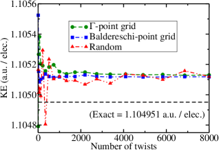
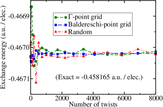
Figure 1: (Color online) Convergence of the calculated KE per electron (top panel) and exchange energy per electron (bottom panel) of a 338-electron simulation cell of HEG at $r_{s}=1$ a.u. as a function of the number of twists for the three different CE twist-averaging methods described in the text. Because of the finite size of the simulation cell, the calculated KE and exchange energy do not converge to their exact infinite-system limits as the number of twists increases: the KE shows a small positive bias and the exchange energy a large negative bias.

kinetic and exchange energies of a face-centered cubic (FCC) simulation cell of HEG containing 338 electrons at $r_{s}=1$ a.u., calculated using sets of twists of various sizes generated in all three ways. As for insulators, energies calculated using random twist sampling converge slowly as the number of twists increases. The most rapid convergence is again obtained with a uniform Monkhorst-Pack grid of twists centered on the Baldereschi point of the simulation-cell Brillouin zone. The twists on a $\Gamma$-point Monkhorst-Pack belong to stars of symmetry-equivalent twists yielding identical energies. The symmetry can be used to reduce the number of trial wave functions that have to be constructed, optimized and stored per twist, but does not decrease the total number of Monte Carlo samples required to obtain a given statistical error and does not affect the conclusion that the Baldereschi-point grid is the most efficient. Because the simulation cell only contains 338 electrons, the KE and exchange energy do not converge to their infinite-system limits as the number of twists increases. The small positive error in the calculated KE is an artifact of the CE twist-averaging algorithm, as discussed in Sec. II.4, and disappears when GCE twist averaging is used. KE’s in QMC simulations suffer from much larger finite-size errors due to long-ranged correlations (see Sec. II.10), but these are absent in HF theory. The large negative finite-size error in the exchange energy is not caused by the CE twist-averaging algorithm and is not removed by GCE averaging, but arises from the compression of the exchange hole into the simulation cell.

Figure 2 shows the convergence with

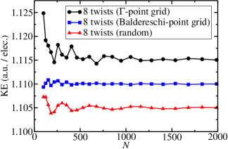
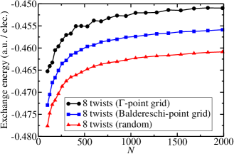
Figure 2: (Color online) Convergence of the calculated KE per electron (top panel) and exchange energy per electron (bottom panel) of a HEG at $r_{s}=1$ a.u. as a function of $N$ for the three different CE twist-averaging methods described in the text, each with eight twists. The $\Gamma$-point and Baldereschi-point results have been offset for clarity.

system size of the CE twist-averaged HF KE and exchange energies of a HEG at $r_{s}=1$ a.u. in an FCC simulation cell, calculated using sets of twists generated in all three ways. To highlight the differences between the three methods, we have used only eight twists in each case. Energies calculated using the uniform grid of twists centered on $\Gamma$ converge the most slowly because of the large fluctuations that occur as the size of the simulation cell increases and shells of symmetry-equivalent ${\bf k}_{s}+{\bf G}_{s}$ vectors cross the Fermi surface. Energies calculated using a random sampling of twists converge more rapidly with system size (although less rapidly with number of twists). Yet again, the best approach uses a uniform grid of twists centered on the Baldereschi point of the simulation-cell Brillouin zone.

Figure 3 shows the error in the

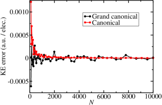
Figure 3: (Color online) System-size dependence of the twist-averaged KE per electron of a HEG at $r_{s}=1$ a.u. in the CE and GCE. All calculations used a random sampling of 5120 twists.

twist-averaged HF KE calculated with a very large set of random twists, using both the CE and GCE. The systematic bias in the CE average disappears when GCE averaging is used, but the large fluctuations in the GCE results outweigh the bias for all but the smallest simulation cells. These fluctuations arise from the variations in electron number inherent in the GCE method. Most QMC simulations are likely to use many fewer twists, rendering the GCE fluctuations even worse, so CE averaging is the more promising method despite the bias. Figure 4 shows the bias in the CE-twist-averaged

Figure 4: Bias in the KE per electron of a HEG at $r_{s}=1$ a.u. as a function of $N$, calculated using 5120 randomly chosen twists in the CE. The power-law fit yields a bias proportional to $N^{-1.32}$.

KE as a function of $N$. The power-law fit shows that the bias per electron decreases relatively slowly with system size, scaling roughly as $N^{-4/3}$, as noted by Lin et al.lin_twist_2001

IV Comparison of the MPC interaction with the finite-size correction to the Ewald energy

If the XC hole can be assumed to have converged to its infinite-system form then both the MPC interaction and the finite-size correction of Eq. (25) are good solutions to the problem of finite-size effects in the XC energy of a cubic system. For low-symmetry systems the MPC interaction should continue to be a good solution, whereas the correction to the Ewald energy cannot be applied straightforwardly. On the other hand, if the simulation cell is too small to contain the infinite-system XC hole, but the SF is known analytically at small $k$, then this information can be included in the XC correction but not the MPC interaction, so the XC correction may work better. In practice the difference between the MPC energy and the corrected Ewald energy for cubic interacting systems is very small when the Ewald interaction is used to generate the configuration distribution, as demonstrated by the data shown for 3D HEGs at three different densities in Table 1. In each case the difference of MPC and Ewald energies is approximately equal to (but slightly greater than) $\Delta V_{\rm Ew}$.

$r_{s}$	$N$	$(E_{\rm MPC}-E_{\rm Ewald})/N$    (a.u. / elec.)		$\Delta V_{\rm Ew}/N$ (a.u. / elec.)		%age difference
1	54	$0$.	$007\,81(1)$	$0$.	$008\,02$	2.6(1)%
1	102	$0$.	$004\,137(9)$	$0$.	$004\,245$	2.5(2)%
1	226	$0$.	$001\,89(1)$	$0$.	$001\,92$	1.6(5)%
3	54	$0$.	$001\,551(4)$	$0$.	$001\,543$	0.5(3)%
3	102	$0$.	$000\,802(2)$	$0$.	$000\,817$	1.8(2)%
3	226	$0$.	$000\,365(1)$	$0$.	$000\,369$	1.1(3)%
10	54	$0$.	$000\,242(1)$	$0$.	$000\,254$	4.7(4)%
10	102	$0$.	$000\,131\,9(4)$	$0$.	$000\,134\,2$	1.7(3)%
10	226	$0$.	$000\,060\,5(7)$	$0$.	$000\,060\,6$	0(1)%

Table 1: Difference between total energies per electron evaluated using the MPC and Ewald interactions in twist-averaged DMC calculations for 3D paramagnetic HEGs at three different densities. The Ewald energy is used in the branching factor in the DMC simulation, so that the configuration distribution appropriate for the Ewald interaction is used in all cases. The DMC time steps were 0.003, 0.03, and 0.3 a.u. at $r_{s}=1$, 3, and 10 a.u., respectively, and the target population was more than 400 configurations in each case. Twist angles were sampled randomly. At each density it was verified that the DMC energy did not change when the time step was halved, the configuration population was doubled, and the number of post-twist-change equilibration steps was quadrupled. The finite-size correction to the Ewald energy [Eq. (26)] is shown for comparison.

It is shown in Appendix A that the long range of the exchange hole causes the MPC energy to be slowly convergent when the interactions are treated within the HF approximation. The finite-size correction constructed using the known small-$k$ behavior of the HF SF therefore performs better than the MPC interaction in HF calculations.

By the variational principle, the expectation value of the MPC Hamiltonian with respect to the Ewald ground-state wave function is greater than the expectation value of the MPC Hamiltonian with respect to the MPC ground-state wave function. The MPC energy obtained using DMC with the Ewald energy in the branching factor is therefore likely to be overestimated, and vice versa. An example of this effect is shown in Table 2. When the Ewald interaction is used in the branching factor, the difference between the MPC and Ewald energies is given by $\Delta V_{\rm Ew}$. However, when the MPC interaction is used, the difference is less than $\Delta V_{\rm Ew}$. These results suggest that the MPC interaction distorts the XC hole in a finite system, while the Ewald interaction gives a better shaped hole, although the interaction with the hole is not quite right. We have directly verified that this is the case for a HEG at $r_{s}=3$ a.u., as can be seen in Fig. 5. The Ewald XC hole converges to its infinite-system form much more rapidly than the MPC hole. The likely reason for this behavior is that the MPC Hamiltonian does not include corrections for finite-size errors in the KE.

	Ewald propagation				MPC propagation
$N$	$E_{\rm Ew}$   /N (a.u. / elec.)		$E_{\rm MPC}/N$ (a.u. / elec.)		$E_{\rm Ew}/N$    (a.u. / elec.)		$E_{\rm MPC}/N$ (a.u. / elec.)
54	$-0$.	$068\,69(6)$	$-0$.	$067\,15(6)$	$-0$.	$068\,18(6)$	$-0$.	$067\,36(6)$
102	$-0$.	$067\,62(3)$	$-0$.	$066\,82(3)$	$-0$.	$067\,68(6)$	$-0$.	$067\,15(6)$
226	$-0$.	$067\,06(4)$	$-0$.	$066\,61(4)$	$-0$.	$066\,85(5)$	$-0$.	$066\,77(5)$

Table 2: Total energies evaluated using Ewald and MPC interactions for 3D paramagnetic HEGs at $r_{s}=3$ a.u. The results were obtained in twist-averaged DMC calculations, as described in the caption to Table 1. The Ewald energy was used in the branching factor in the results labeled “Ewald propagation,” while the MPC energy was used in the results labeled “MPC propagation” (i.e., the XC hole was appropriate for the Ewald and MPC interactions, respectively). $E_{\rm Ew}$ and $E_{\rm MPC}$ refer to the interaction (Ewald and MPC, respectively) used in the local energies that were averaged to obtain the DMC energy.

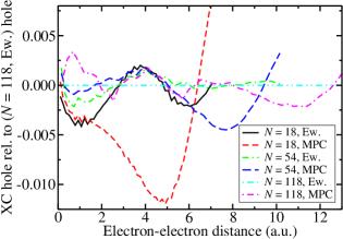
Figure 5: (Color online) System-averaged XC hole in a 3D paramagnetic HEG of density parameter $r_{s}=3$ a.u. at different system sizes relative to the XC hole in a 118-electron HEG with the Ewald interaction. The Ewald and MPC interactions were used to generate the configuration distributions. Twist-averaged VMC and DMC XC holes $\rho_{\rm xc}^{\rm VMC}(r)$ and $\rho_{\rm xc}^{\rm DMC}(r)$ were calculated, and the final XC hole was obtained using the extrapolated estimate $\rho_{\rm xc}(r)\approx 2\rho_{\rm xc}^{\rm DMC}(r)-\rho_{\rm xc}^{\rm VMC}(r)$. The error in the extrapolated estimate is second order in the error in the trial wave function.foulkes_2001

V Nonanalytic behavior at ${\bf k}={\bf 0}$

V.1 Examples of nonanalytic behavior at ${\bf k}={\bf 0}$

The XC correction discussed in Sec. II.9 works well for interacting systems of cubic symmetry. In other cases, however, the theory cannot be applied straightforwardly. We give two examples.

For a general interacting system, the SF at small $k$ can be written as $S({\bf k})=(1/2){\bf k}^{T}W^{\prime}{\bf k}$ for some tensor $W^{\prime}$. If the system has cubic symmetry then $W^{\prime}$ is proportional to the identity matrix and $\lim_{{\bf k}\rightarrow{\bf 0}}S({\bf k})/k^{2}$ is well-defined. Otherwise, this limit is undefined and it is not possible to add the ${\bf G}_{s}={\bf 0}$ term to the sum in Eq. (24).

Within HF theory, $S({\bf k})=\lambda k+O(k^{3})$ at small $k$, where $\lambda$ is a constant.giuliani The limit of $S({\bf k})/k^{2}$ as ${\bf k}\rightarrow{\bf 0}$ is therefore undefined. Again the approach discussed in Sec. II.9 cannot be applied.

V.2 Removing the problematic part of the SF

Suppose that $S({\bf k})/k^{2}$ is singular or otherwise ill-defined at ${\bf k}={\bf 0}$, but that its small-${\bf k}$ behavior is known and is roughly independent of $N$. We can then introduce a model “structure factor” $S_{b}({\bf k})$ that incorporates the nonanalytic behavior and define $S_{a}({\bf k})=S({\bf k})-S_{b}({\bf k})$, so that $\lim_{{\bf k}\rightarrow{\bf 0}}S_{a}({\bf k})/k^{2}$ is well defined. Starting from Eq. (24) and applying the Poisson summation formulafootnote:poisson to terms involving $S_{a}$ only yields

$$\Delta V_{\rm Ew}=\frac{N}{2}\left(\frac{4\pi}{\Omega}\lim_{{\bf k}\rightarrow{\bf 0}}\frac{S_{a}({\bf k})}{k^{2}}+\frac{1}{(2\pi)^{3}}\int_{k<\infty}v_{E}(k)S_{b}({\bf k})\,d{\bf k}-\frac{1}{\Omega}\sum_{{\bf G}_{s}\neq{\bf 0}}v_{E}(G_{s})S_{b}({\bf G}_{s})\right)-\frac{N}{2}\sum_{{\bf R}_{s}\neq{\bf 0}}\int_{r^{\prime}<\infty}\frac{S_{a}({\bf r}^{\prime})}{|{\bf R}_{s}-{\bf r}^{\prime}|}\,d{\bf r}^{\prime},$$ (38)

where $S_{a}({\bf r})$ is a localized charge distribution analogous to $S_{\rm loc}({\bf r})$ and all convergence factors have been omitted. Since the ${\bf k}\rightarrow{\bf 0}$ behavior of $S_{a}({\bf k})/k^{2}$ is known, and provided that $S_{b}({\bf k})$ has a simple enough form, all three terms within the large parentheses in Eq. (38) can be evaluated straightforwardly. Moreover, since $S_{a}({\bf k})$ is well-behaved as ${\bf k}\rightarrow{\bf 0}$, $S_{a}({\bf r})$ lacks the long-ranged tail present in $S_{\rm loc}({\bf r})$; the summation in the final term on the right-hand side of Eq. (38) therefore converges rapidly and should be small. This term is omitted from the approximate expressions for the finite-size correction obtained below, and therefore represents the error in these approximations.

The finite-size correction obtained by evaluating all except the final term on the right-hand side of Eq. (38) is accurate when $S_{a}({\bf k})=S({\bf k})-S_{b}({\bf k})$ is smooth, implying that $S_{a}({\bf r})$ is short ranged. The model structure factor $S_{b}({\bf k})$ should therefore match the nonanalytic behavior of $S({\bf k})$ as closely as possible. It is also sensible, although less important, to ensure that $S({\bf k})-S_{b}({\bf k})$ is small. In practice, although $S({\bf k})\rightarrow 1$ as $k\rightarrow\infty$, the correction is most easily evaluated if $S_{b}({\bf k})\rightarrow 0$ as $k\rightarrow\infty$. A natural way of accomplishing this is to include a Gaussian function $\exp(-\alpha k^{2})$ as a factor. The parameter $\alpha$ should be small enough that the Gaussian changes little on the scale of the Fermi wave vector. In fact, although the reciprocal space summation and integration diverge in the $\alpha\rightarrow 0$ limit, their difference converges rapidly. One can therefore maximize the smoothness of $S_{a}({\bf k})$ by decreasing $\alpha$ until the calculated value of the correction has converged.

A plausible alternative methodfin_chiesa for dealing with leading-order nonanalyticities in $S({\bf k})/k^{2}$ at ${\bf k}={\bf 0}$ is to replace the missing ${\bf G}_{s}={\bf 0}$ term in the sum over ${\bf G}_{s}$ in Eq. (18) with an integral of $v_{E}(k)S({\bf k})$ over a sphere of volume $(2\pi)^{3}/\Omega$. This approach may be cast into the framework discussed above by choosing $S_{b}({\bf k})=S({\bf k})\Theta(Q-k)$, where $Q$ is the radius of the sphere of volume $(2\pi)^{3}/\Omega$ and $\Theta(Q-k)$ is a Heaviside step function. The function $S_{a}({\bf k})=S({\bf k})-S_{b}({\bf k})$ is then zero at the origin, so the first term inside the parentheses in Eq. (38) vanishes. Unless the lattice is very asymmetric, $S_{b}({\bf G}_{s})$ is zero for all nonzero ${\bf G}_{s}$, and the third term inside the parentheses in Eq. (38) also vanishes. Hence

$$\Delta V_{\rm Ew}=\frac{N}{2}\left(\frac{1}{(2\pi)^{3}}\int_{k<Q}v_{E}(k)S({\bf k})\,d{\bf k}\right)-\frac{N}{2}\sum_{{\bf R}_{s}\neq{\bf 0}}\int_{r^{\prime}<\infty}\frac{S_{a}({\bf r}^{\prime})}{|{\bf R}_{s}-{\bf r}^{\prime}|}\,d{\bf r}^{\prime}.$$ (39)

In this case, however, the sharp cutoff in $S_{b}({\bf k})$ leads to slowly decaying oscillations in $S_{b}({\bf r})$ and therefore $S_{a}({\bf r})$. These oscillations fall off as $r^{-2}$ and can never be regarded as negligible. Unless $S({\bf k})/k^{2}$ is constant for $k<Q$, in which case this correction is accurate by construction, the neglected real-space term in Eq. (39) is of the same order as the correction itself.

V.3 Finite-size corrections in HF theory

Suppose $S({\bf k})=\lambda k+O(k^{3})$, as is the case for systems of cubic symmetry in HF theory. The divergence of $S({\bf k})/k^{2}$ as ${\bf k}\rightarrow{\bf 0}$ prevents Eqs. (25) and (30) from being used to obtain finite-size corrections. Let $S_{b}({\bf k})=\lambda k\exp(-\alpha k^{2})$. Working in the $\alpha\rightarrow 0$ limit, Eq. (38) becomes

$$\Delta V_{\rm Ew}=\lim_{\alpha\rightarrow 0}\frac{N}{2}\left(\frac{\lambda}{\pi\alpha}-\frac{4\pi\lambda}{\Omega}\sum_{{\bf G}_{s}\neq{\bf 0}}\frac{\exp\left(-\alpha G_{s}^{2}\right)}{G_{s}}\right)+O(N^{-1/3})=\frac{C_{\rm HF}\lambda N}{\Omega^{2/3}}+O(N^{-1/3}),$$ (40)

where $C_{\rm HF}=2.8884$, $2.8372$, and $2.8882$ for FCC, simple cubic (SC), and body-centered cubic (BCC) simulation cells, respectively,footnote:program and we have noted that the $O(k^{3})$ term in $S_{a}({\bf k})=S({\bf k})-S_{b}({\bf k})$ causes $S_{a}({\bf r})$ to fall off as $r^{-6}$, giving the $O(N^{-1/3})$ correction. For a 3D paramagnetic HEG,giuliani $\lambda=(3/4)[\Omega/(3N\pi^{2})]^{1/3}$, so

$$\Delta V_{\rm HF}=\frac{3C_{\rm HF}}{4\pi r_{s}}\left(\frac{N}{4}\right)^{1/3}+O(N^{-1/3}).$$ (41)

An alternative real-space treatment of HF finite-size errors can be found in Appendix A. As shown in Fig. 6, both the real- and reciprocal-space approaches account for most of the HF Coulomb finite-size error, although the reciprocal-space approach performs better because it completely removes the $O(N^{1/3})$ error.

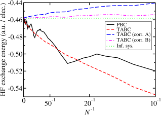
Figure 6: (Color online) HF Ewald exchange energy per electron of a 3D paramagnetic HEG of density parameter $r_{s}=1$ a.u. against particle number $N$ with ${\bf k}_{s}={\bf 0}$ (“PBC”) and twist-averaged boundary conditions within the CE (“TABC”). The corrections of Eqs. (75) and (41) have been applied to the data labeled “TABC (corr. A)” and “TABC (corr. B),” respectively. An FCC simulation cell is used. The uncertainty in the twist-averaged data due to the use of a finite number of twist angles is small compared with the difference between the twist-averaged data and the infinite-system result.

V.4 Finite-size errors in the XC energy of low-symmetry systems

For a general interacting system the SF can be written as

$$S({\bf k})=\sum_{{\rm even}~{}l}\,\,\sum_{m=-l}^{l}S_{lm}(k)k^{l}Y_{lm}(\theta_{\bf k},\phi_{\bf k}),$$ (42)

where $\theta_{\bf k}$ and $\phi_{\bf k}$ are the polar and azimuthal angles of ${\bf k}$ and $Y_{lm}$ is the $(l,m)$-th spherical harmonic. The odd-$l$ components are zero by inversion symmetry. Guided by the RPA, we assume that $S({\bf k})$ is quadratic near ${\bf k}={\bf 0}$, and hence that $S_{00}(k)\propto k^{2}$. If the quadratic form is nonspherical, however, $l=2$ components are also present and $\lim_{{\bf k}\rightarrow{\bf 0}}S({\bf k})/k^{2}$ depends on the direction in which the limit is taken; there is then a point discontinuity at ${\bf k}={\bf 0}$. Equivalently, the $l=2$ component gives rise to the quadrupole moment in $S_{\rm loc}({\bf r})$, which leads to the additional errors discussed in Sec. II.9.

Let

$$S_{b}({\bf k})=\sum_{m=-2}^{2}S_{2m}(0)k^{2}Y_{2m}(\theta_{\bf k},\phi_{\bf k})\exp\left(-\alpha k^{2}\right),$$ (43)

and $S_{a}({\bf k})=S({\bf k})-S_{b}({\bf k})$, where $\alpha$ is such that $S_{b}({\bf k})$ is long-ranged in ${\bf k}$-space compared with the Fermi wave vector. Applying Eq. (38) and taking the limit $\alpha\rightarrow 0$, we find that

$$\Delta V_{\rm Ew}=\frac{N}{2}\left(\frac{4\pi Y_{00}}{\Omega}\lim_{k\rightarrow 0}\frac{S_{00}(k)}{k^{2}}-\frac{4\pi}{\Omega}\sum_{m=-2}^{2}S_{2m}(0)\sum_{{\bf G}_{s}\neq{\bf 0}}Y_{2m}(\theta_{{\bf G}_{s}},\phi_{{\bf G}_{s}})\right)+O(N^{-1/3}).$$ (44)

In particular, it can be seen that the $O(N^{0})$ finite-size correction obtained using the spherically averaged SF is incomplete, and that there is in general another correction of $O(N^{0})$ due to the low symmetry of the simulation cell and the existence of the $l=2$ component. If the XC hole has spherical symmetry, the extra correction is zero regardless of the shape of the simulation cell; if the XC hole does not have spherical symmetry, but the simulation cell does have cubic symmetry, the extra correction is again zero. Hence, if one is simulating a low-symmetry system, it is advisable to choose a simulation cell that is as close to cubic as possible. If this is not possible then one could evaluate the $l=0$ and $l=2$ components of $S({\bf k})$ at ${\bf k}={\bf 0}$, and use Eq. (44) to compute the correction. The $O(N^{-1/3})$ error in Eq. (44) arises from an assumed nonanalytic $O(k^{3})$ term in $S_{a}({\bf r})$.

VI Higher-order corrections to the KE

VI.1 Need to include higher-order corrections

The need to include higher-order finite-size corrections to the KE is demonstrated in Fig. 7, which shows the size dependence of the DMC energy of the 3D HEG. The XC- and KE-corrected Ewald data and the KE-corrected MPC data are in good agreement with each other, as expected. At low density ($r_{s}=10$ a.u.) the corrected data are almost independent of system size, indicating that the finite-size correction formulas are working well. However, at intermediate ($r_{s}=3$ a.u.) and high density ($r_{s}=1$ a.u.) it is clear that the QMC data are overcorrected when only the leading-order KE correction is applied. Since the finite-size correction $\Delta V_{\rm Ew}$ to the interaction energy has been shown to be accurate, the problem must lie in the KE. It is clearly necessary to go beyond leading order when correcting the KE at intermediate and high densities.

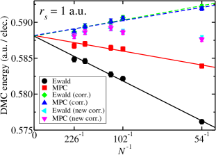
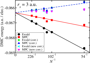
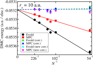
Figure 7: (Color online) DMC total energy per electron against the reciprocal of the number of electrons in 3D paramagnetic HEGs of density parameter $r_{s}=1$ a.u. (top panel), $r_{s}=3$ a.u. (middle panel), and $r_{s}=10$ a.u. (bottom panel). The simulation parameters were as described in the caption of Table 1. The Ewald energy per electron is corrected by the addition of $(\Delta V_{\rm Ew}+\Delta T_{A})/N=\omega_{p}/(2N)$ [“Ewald (corr.)”], while the MPC energy is corrected by the addition of $\Delta T_{A}/N=\omega_{p}/(4N)$ [“MPC (corr.)”]. The corrected Ewald and MPC energies are hard to distinguish because they lie almost on top of each other. The higher-order KE corrections described in Sec. VI.2 ($\Delta T_{B}/N$ plus the single-particle correction) are included in the data sets labeled “(new corr.)”.

The Poisson summation formula can be used to demonstrate that higher-order terms are more important in the KE than the Ewald energy. If we assume that the XC hole is well localized within the simulation cell and that $\lim_{{\bf k}\rightarrow{\bf 0}}k^{2}u(k)$ exists, the finite-size correction to the KE may be obtained from Eq. (36) as

$$\Delta T = \frac{N}{4}\left(\frac{1}{(2\pi)^{3}}\int_{k<\infty}k^{2}u({\bf k})[S({\bf k})-1]\,d{\bf k}-\frac{1}{\Omega}\sum_{{\bf G}_{s}\neq{\bf 0}}G_{s}^{2}u({\bf G}_{s})[S({\bf G}_{s})-1]\right)$$ (45)

$$= \frac{N}{4}\left(-\frac{1}{\Omega}\lim_{{\bf k}\rightarrow{\bf 0}}k^{2}u({\bf k})-\sum_{{\bf R}_{s}\neq{\bf 0}}L({\bf R}_{s})\right),$$ (46)

where we have used the Poisson summation formulafootnote:poisson and

$$L({\bf r})=-\nabla^{2}\int_{r^{\prime}<\infty}u({\bf r}-{\bf r}^{\prime})\rho_{\rm xc}({\bf r}^{\prime})\,d{\bf r}^{\prime}$$ (47)

is the inverse Fourier transform of $k^{2}u({\bf k})[S({\bf k})-1]$.

The leading-order behavior of the two-body Jastrow factor of a HEG at small $k$ isgaskell $u(k)=-4\pi\left(A/k^{2}+B/k\right)$ within the RPA. Hence, at large $r$, $u(r)=-A/r-2B/(\pi r^{2})$ and so $\nabla^{2}u({\bf r})=-4B/(\pi r^{4})$ for $r\neq 0$. The finite-size correction to the KE is therefore

$$\Delta T=\frac{N\pi A}{\Omega}-\frac{NB}{\pi}\sum_{{\bf R}_{s}\neq{\bf 0}}\int_{r<\infty}\frac{\rho_{\rm xc}({\bf r})\,d{\bf r}}{|{\bf R}_{s}-{\bf r}|^{4}}.$$ (48)

The first term is the correction of Eq. (37), while the second term gives an additional correction that falls off slowly as $N^{-1/3}$. So, even in the case of the HEG, where the next-to-leading-order correction to the Ewald energy falls off as $N^{-1}$, higher-order corrections to the KE may be important.

The additional KE correction is due to the discontinuous gradient of $k^{2}u({\bf k})$ at ${\bf k}={\bf 0}$. A similar approach to that developed in Sec. V.2 can be used to eliminate the leading-order nonanalytic contributions to the long-ranged part of $\nabla^{2}u({\bf r})$. Define $F({\bf k})=k^{2}u({\bf k})[S({\bf k})-1]$ and write $F({\bf k})=F_{a}({\bf k})+F_{b}({\bf k})$, where $F_{b}({\bf k})$ contains the $O(k)$ contribution to $-k^{2}u({\bf k})$ [as well as any anisotropic $O(k^{0})$ terms], and is smooth and long-ranged in ${\bf k}$-space. Then

$$\Delta T=\frac{N}{4}\left(\frac{1}{\Omega}\lim_{{\bf k}\rightarrow{\bf 0}}F_{a}({\bf k})+\frac{1}{(2\pi)^{3}}\int_{k<\infty}F_{b}({\bf k})\,d{\bf k}-\frac{1}{\Omega}\sum_{{\bf G}_{s}\neq{\bf 0}}F_{b}({\bf G}_{s})\right)+\frac{N}{4}\sum_{{\bf R}_{s}\neq{\bf 0}}F_{a}({\bf R}_{s}).$$ (49)

Note that, as shown in Sec. III, the bias due to residual CE twist-averaged single-particle KE errors also falls off as $N^{-1/3}$. If we include higher-order corrections for the neglect of long-ranged correlations, we should also correct for the residual error in the twist-averaged energy.

VI.2 Higher-order KE corrections

Gaskellgaskell has derived the following expression for the small-$k$ limit of $u({\bf k})$ for the 3D HEG within the RPA:

$$u(k) = -\frac{\Omega}{N}\left\{-\frac{1}{2S_{0}(k)}+\left[\frac{1}{4S_{0}^{2}(k)}+\left(\frac{v_{E}(k)N}{\Omega\omega_{p}}\right)^{2}\right]^{1/2}\right\}$$ (50)

$$\equiv -4\pi\left[\frac{A}{k^{2}}+\frac{B}{k}\right]+O(k^{0}),$$ (51)

where

$$S_{0}(k)=\sum_{\sigma}\frac{N_{\sigma}}{N}\left[\frac{3k}{4k_{{\rm F}\sigma}}-\frac{k^{3}}{16k_{{\rm F}\sigma}^{3}}\right]$$ (52)

is the HF SF, $k_{{\rm F}\sigma}=\left(6\pi^{2}N_{\sigma}/\Omega\right)^{1/3}$ is the Fermi wave vector for particles of spin $\sigma$, $N_{\sigma}$ is the number of particles of spin $\sigma$, and

$$A = \frac{1}{\omega_{p}}=\sqrt{\frac{r_{s}^{3}}{3}}$$ (53)

$$B = -\frac{2r_{s}^{2}}{3}\left(\frac{2\pi}{3}\right)^{1/3}\left[(1+\zeta)^{2/3}+(1-\zeta)^{2/3}\right]^{-1},$$ (54)

where $\zeta=(N_{\uparrow}-N_{\downarrow})/N$ is the spin polarization.

Let $F_{b}(k)=4\pi Bk\exp(-\alpha k^{2})$. This satisfies the requirements for $F_{b}$ given in Sec. VI.1, provided $\alpha$ is small. Then, by Eq. (49) in the limit $\alpha\rightarrow 0$,

$$\Delta T = \frac{N}{4}\left(\frac{4\pi A}{\Omega}+\frac{B}{\pi\alpha^{2}}-\frac{4\pi B}{\Omega}\sum_{{\bf G}_{s}\neq{\bf 0}}G_{s}\exp\left(-\alpha G_{s}^{2}\right)\right)+O(N^{-2/3})$$ (55)

$$= \frac{N\pi A}{\Omega}+\frac{C_{\rm 3D}NB}{\Omega^{4/3}}+O(N^{-2/3})$$

$$= \frac{\omega_{p}}{4}-\frac{C_{\rm 3D}}{2\pi r_{s}^{2}(2N)^{1/3}}\left[(1+\zeta)^{2/3}+(1-\zeta)^{2/3}\right]^{-1}+O(N^{-2/3})\equiv\Delta T_{A}+\Delta T_{B}+O(N^{-2/3}),$$ (56)

where $C_{\rm 3D}=5.083$, $5.264$, and $5.086$ for FCC, SC, and BCC simulation cells, respectively. The $O(N^{-2/3})$ error arises from the $O(r^{-3})$ term in $u(r)$ at large $r$.

The relative importance of the corrections for typical system sizes at three different densities is shown in Table 3. The residual CE twist-averaged single-particle KE error is generally greater than $\Delta T_{B}$. This error can be estimated within HF theory.footnote_effmass For real systems, the “infinite-system” HF energy would have to be evaluated in a large, finite calculation. The effect of adding higher-order corrections (including the correction for the residual single-particle error) to the energy of a 3D HEG is demonstrated in Fig. 7. The finite-size behavior of the QMC data is clearly greatly improved at $r_{s}=1$ and 3 a.u.

		KE correction (a.u. / elec.)
$r_{s}$ (a.u.)	$N$	SP corr.		$\Delta T_{A}/N$		$\Delta T_{B}/N$
1	54	$-0$.	$002\,8$	$0$.	$008\,0$	$-0$.	$001\,6$
1	130	$-0$.	$000\,65$	$0$.	$003\,33$	$-0$.	$000\,48$
3	54	$-0$.	$000\,31$	$0$.	$001\,54$	$-0$.	$000\,17$
3	130	$-0$.	$000\,072$	$0$.	$000\,641$	$-0$.	$000\,054$
10	54	$-0$.	$000\,027$	$0$.	$000\,254$	$-0$.	$000\,015$
10	130	$-0$.	$000\,006$	$0$.	$000\,105$	$-0$.	$000\,005$

Table 3: Magnitude of different components of the finite-size correction to the KE per electron of a 3D paramagnetic HEG at different density parameters $r_{s}$ and system sizes $N$ in an FCC cell. The correction for residual single-particle errors after twist averaging in the CE (“SP corr.”) is estimated as the difference between the infinite-system HF KE and the twist-averaged HF KE for the finite system.

For real systems we do not usually have an analytic result for the small-$k$ behavior of $u({\bf k})$. However, we have flexible forms of $u({\bf r})$ that can be optimized within QMC. By fitting a suitable functional form to the QMC-optimized $u$, we can extrapolate to the ${\bf k}={\bf 0}$ limit. We suggest that Eq. (51) be fitted to the QMC $u(G_{s})$ at the first two stars of nonzero ${\bf G}_{s}$ vectors, and that Eq. (55) should then be used to evaluate the KE correction.

VI.3 Low-${\bf k}$ behavior of the Fourier-transformed two-body Jastrow factor

The Fourier transform of the two-body Jastrow factor of a 3D paramagnetic HEG at $r_{s}=3$ a.u. is shown in Fig. 8. The Jastrow factor consisted of polynomial and plane-wave expansions in electron-electron separation,ndd_jastrow which were optimized by variance minimizationumrigar_1988a ; ndd_newopt followed by energy minimization.umrigar_emin As expected, the form of $u({\bf k})$ is largely independent of the number of electrons, and the small-$k$ behavior is well-described both by the RPA of Eq. (50) and by the first two terms of the power-series expansion, Eq. (51). The RPA expression for the two-body Jastrow factor does not satisfy the Kato cusp conditionskato_pack and hence becomes unreliable at large $k$. The small-$k$ behavior of $u({\bf k})$ for 54- and 226-electron HEGs is shown in Fig. 9. It can be seen that the fit of the two-term RPA expansion to the QMC-optimized Jastrow factor is a fairly good approximation to the analytic RPA form within a sphere of volume $(2\pi)^{3}/\Omega$, but that the fitted three-term RPA expansion is badly behaved, because one is simply fitting to the noise in the $u({\bf G}_{s})$ data. This is reflected in the corresponding results for the KE correction shown in Table 4. The corrections obtained with the fitted two-term expansion are close to the analytic KE correction (leading-order and next-to-leading order terms). The leading-order correction can be thought of as being calculated on the assumption that $k^{2}u(k)$ is constant over the integration regions shown in Fig. 9, which is clearly inappropriate, and leads to the overcorrection for $N=54$ electrons. The fitted three-term RPA expansion also gives an overcorrection. For HEGs, the analytic results given in Sec. VI.2 should of course be used.

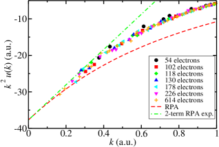
Figure 8: (Color online) Fourier transform of the fully optimized two-body Jastrow factor for a paramagnetic 3D HEG at $r_{s}=3$ a.u. and different system sizes. For comparison, the RPA expression of Eq. (50) and the two-term RPA expansion [Eq. (51)] are shown.

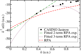
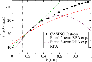
Figure 9: (Color online) Two-body Jastrow factor for a paramagnetic 3D HEG at $r_{s}=3$ a.u. with 54 electrons (top panel) and 226 electrons (bottom panel). The Jastrow factors are as in Fig. 8. The RPA expression of Eq. (50) is plotted, as are fits of the two- and three-term RPA expansions [Eq. (51) and Eq. (51) with an extra term $-4\pi C$]. The fits were made to the QMC-optimized $u$ at the first two and first three stars of ${\bf G}_{s}$ vectors, respectively. The dotted line indicates the radius of the sphere whose volume is $(2\pi)^{3}/\Omega$.

Method	$N$	$A$ (a.u.)		$\Delta T$ (a.u.)
Analytic RPA	$54$	$3$		$0$	$.073\,9$
Analytic 1-term exp.	Any	$3$		$0$	$.083\,2$
Fitted 2-term exp.	$54$	$3$	$.22$	$0$	$.079\,1$
Fitted 3-term exp.	$54$	$4$	$.41$	$0$	$.097\,6$
Analytic RPA	$226$	$3$		$0$	$.077\,5$
Fitted 2-term exp.	$226$	$3$	$.15$	$0$	$.081\,0$
Fitted 3-term exp.	$226$	$3$	$.53$	$0$	$.086\,9$

Table 4: Finite-size correction to the KE of a paramagnetic HEG of density parameter $r_{s}=3$ a.u., calculated using different two-body Jastrow factors. The value of $A=3$ corresponds to $1/\omega_{p}$; see Eq. (54). We compare analytic results with those obtained by fitting to the QMC-optimized two-body Jastrow factors shown in Fig. 9. The “Analytic RPA” form is that of Eq. (50), the “3-term exp.” is that of Eq. (51) with an extra term $-4\pi C$, the “2-term exp.” is Eq. (51), and the “1-term exp.” is Eq. (51) with $B=0$.

VII Finite-size corrections in 2D systems

VII.1 XC energy in 2D

Consider a 2D-periodic system with simulation-cell area $P$. For a sufficiently symmetric system, $S({\bf k})=\gamma k^{3/2}+O(k^{2})$.pines Hence $\lim_{{\bf k}\rightarrow{\bf 0}}v_{E}(k){S}({\bf k})=2\pi\lim_{{\bf k}\rightarrow{\bf 0}}{S}(k)/k=0$. So the 2D analog of Eq. (30) is

$$\Delta V_{\rm Ew}=-\frac{N}{2}\sum_{{\bf R}_{s}\neq{\bf 0}}\phi_{\rm loc}({\bf R}_{s}).$$ (57)

In a 2D HEG the nonoscillatory XC hole is relatively long-ranged due to the reduced screening, decaying as $\rho_{\rm xc}(r)=-\tilde{\Lambda}r^{-7/2}$, where $\tilde{\Lambda}$ is a constant.gorigiorgi_2D Hence the XC charge outside radius $r$ is $-4\pi\tilde{\Lambda}/(3r^{3/2})$ and the leading (monopolar) contribution to $\phi_{\rm loc}({\bf r})$ is proportional to $r^{-5/2}$ at large $r$. [The dipole moment of the electron and its XC hole is zero, while the quadrupolefootnote:2D_quadrupole contribution to $\phi_{\rm loc}({\bf r})$ is proportional to $r^{-3}$.] Hence

$$\Delta V_{\rm Ew}\propto-\frac{N}{2}\sum_{{\bf R}_{s}\neq 0}R_{s}^{-5/2}=O(N^{-1/4}),$$ (58)

since the length of every simulation-cell lattice vector ${\bf R}_{s}$ appearing in the summation is proportional to $\sqrt{N}$. Unlike the 3D case, therefore, $\Delta V_{\rm Ew}\rightarrow 0$ as $N\rightarrow\infty$. This conclusion was also reached, using a different approach, by Wood et al.wood

To obtain the leading-order correction to the XC energy, we use the method of Sec. V.2. Let $S_{b}(k)=\gamma k^{3/2}\exp(-\alpha k^{2})$. Then, by the 2D analog of Eq. (38),

$$\Delta V_{\rm Ew} = \frac{N}{2}\left(0+\frac{1}{(2\pi)^{2}}\int_{0}^{\infty}v_{E}(k)S_{b}(k)\times 2\pi k\,dk-\frac{1}{P}\sum_{{\bf G}_{s}\neq{\bf 0}}v_{E}(G_{s})S_{b}(G_{s})\right)+O(N^{-1/2})$$ (59)

$$= \frac{N}{2}\left(\frac{\Gamma(5/4)\gamma}{2\alpha^{5/4}}-\frac{2\pi\gamma}{P}\sum_{{\bf G}_{s}\neq{\bf 0}}\sqrt{G_{s}}\exp\left(-\alpha G_{s}^{2}\right)\right)+O(N^{-1/2})$$

$$= \frac{C_{\rm 2D}N\gamma}{P^{5/4}}+O(N^{-1/2}),$$

where $C_{\rm 2D}=3.9852$ and 3.9590 for square and hexagonal cells, respectively, and the $\alpha\rightarrow 0$ limit was taken in the final step. The $O(N^{-1/2})$ error is due to the quadrupole moment of $S_{a}({\bf r})=S({\bf r})-S_{b}({\bf r})$. For a 2D HEG,gorigiorgi_2D $\gamma=2^{-3/4}r_{s}^{-1/2}$. Hence

$$\Delta V_{\rm Ew}=\frac{C_{\rm 2D}}{2\pi r_{s}^{3}}\left(\frac{2}{\pi N}\right)^{1/4}+O(N^{-1/2}).$$ (60)

This correction falls off very rapidly with $r_{s}$.

VII.2 KE in 2D

For a symmetric 2D-periodic system,tanatar_1989 $u(k)=-ak^{-3/2}+O(k^{-1})$ and $S(k)=\gamma k^{3/2}+O(k^{2})$. Hence, proceeding as in Sec. VI.1, we have $F(k)=k^{2}u(k)[S(k)-1]=ak^{1/2}+O(k)$. Let $F_{b}(k)=ak^{1/2}\exp(-\alpha k^{2})$. Then, by the 2D analog of Eq. (49),

$$\Delta T=\frac{N}{4}\left(0+\frac{\Gamma(5/4)a}{4\pi\alpha^{5/4}}-\frac{a}{P}\sum_{{\bf G}_{s}\neq{\bf 0}}\sqrt{G_{s}}\exp\left(-\alpha G_{s}^{2}\right)\right)+O(N^{-1/2})=\frac{C_{\rm 2D}Na}{4\pi P^{5/4}}+O(N^{-1/2}),$$ (61)

where the $\alpha\rightarrow 0$ limit was taken in the final step.

For a 2D HEG the HF SF isgiuliani

$$S_{0}(k)=\sum_{\sigma}\frac{2N_{\sigma}}{\pi N}\left[\sin^{-1}\left(\frac{k}{2k_{{\rm F}\sigma}}\right)+\frac{k}{2k_{{\rm F}\sigma}}\sqrt{1-\left(\frac{k}{2k_{{\rm F}\sigma}}\right)^{2}}\right],$$ (62)

where the Fermi wave vector for electrons of spin $\sigma$ is $k_{{\rm F}\sigma}=\sqrt{4\pi N_{\sigma}/P}$. The small-$k$ limit of the two-body Jastrow factor within the RPA istanatar_1989

$$u(k)=-\frac{P}{N}\left\{\frac{-1}{2S_{0}(k)}+\left[\frac{1}{[2S_{0}(k)]^{2}}+\frac{Nv_{E}(k)}{Pk^{2}}\right]^{1/2}\right\}=-\frac{\sqrt{2}\pi r_{s}}{k^{3/2}}+O(k^{-1}).$$ (63)

Hence

$$\Delta T=\frac{C_{\rm 2D}}{\pi(\pi N)^{1/4}(2r_{s})^{3/2}}+O(N^{-1/2}).$$ (64)

For real systems, we suggest that the Fourier transform of the two-body Jastrow factor be fitted to $u(k)=-a/k^{3/2}-b/k$ using the first two nonzero stars of simulation-cell ${\bf G}_{s}$ vectors. Equation (61) should then be used to calculate the KE correction.

VII.3 Effectiveness of 2D KE correction

We illustrate the effectiveness of the KE corrections in a 2D HEG at low density in Fig. 10. The XC correction [Eq. (60)] is negligibly small at this density. However it is clear that applying finite-size corrections to the KE alone is not sufficient to obtain accurate results. The MPC interaction gives significantly smaller finite-size errors than the Ewald interaction; nevertheless it is clear that extrapolation is necessary.

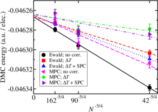
Figure 10: (Color online) Twist-averaged DMC energy per electron against system size for a 2D paramagnetic HEG of density parameter $r_{s}=20$ a.u. The trial wave function was of Slater-Jastrow-backflow form,backflow the target population was 1536 configurations, and the DMC energies have been extrapolated to zero time step. In each case the Ewald interaction was used in the DMC branching factor. “Ewald” and “MPC” indicate the interaction used to calculate the local energies. $\Delta T$ is given in Eq. (64), respectively, and “SPC” denotes the single-particle correction to the KE (the difference of the infinite-system and CE twist-averaged finite-system HF KE’s).

VIII Formulas for finite-size extrapolation

VIII.1 Finite-size extrapolation

In nearly all QMC studies of condensed matter to date it has been necessary to extrapolate energy data to infinite system size by means of an assumed relationship between energy and particle number. These formulas contain free parameters, including the infinite-system energy, which are determined by a fit to the QMC data. Despite the existence of sophisticated methods for treating finite-size errors, it is likely that some form of extrapolation will continue to be necessary for accurate work. In this section we analyze the performance of fitting formulas that have been proposed in the literature and consider how best to extrapolate QMC energies to infinite system size.

Throughout this section we denote the QMC energy per electron of an $N$-electron system by $e(N)$ and we denote the HF energy, KE, and interaction energy per electron by $e_{\rm HF}(N)$, $t_{\rm HF}(N)$, and $v_{\rm HF}(N)$, respectively. We assume that the same ${\bf k}_{s}$ is used in both the QMC and HF calculations (or that twist averaging is applied in both cases).

VIII.2 Finite-size extrapolation formulas for the HEG

The exact size-dependence of the HF energy of the fluid phase of the HEG is

$$e_{\rm HF}(\infty)=e_{\rm HF}(N)+\Delta t_{\rm HF}(N)+\Delta v_{\rm HF}(N),$$ (65)

where $\Delta t_{\rm HF}(N)=t_{\rm HF}(\infty)-t_{\rm HF}(N)$ and $\Delta v_{\rm HF}(N)=v_{\rm HF}(\infty)-v_{\rm HF}(N)$. The forms of $\Delta t_{\rm HF}(N)$ and $\Delta v_{\rm HF}(N)$ for a 3D paramagnetic HEG can be seen in Fig. 1. Both are oscillatory functions of $N$ due to single-particle finite-size errors. The fluctuations in the exchange energy and the KE are strongly correlated, although those in the KE are larger. For further discussion of the single-particle finite-size errors in HF theory, see Sec. II.4 and Ref. lin_twist_2001, . There is also a systematic error in the HF exchange energy, caused by the compression of the exchange hole, as discussed in Appendix A. For a Wigner crystal, Ceperleyceperley_1978 suggested the fitting form

$$e(\infty)=e(N)+\frac{c}{r_{s}^{3/2}N^{3/d}},$$ (66)

where $d$ is the dimensionality and $c$ is roughly independent of $r_{s}$. This is consistent with the form of the 3D XC correction [Eq. (25)] and the leading-order correction to the KE [Eq. (37)]. For an interacting Fermi fluid, Ceperleyceperley_1978 suggested that the HF extrapolation is appropriate at small $r_{s}$, while the Wigner-crystal extrapolation is more reasonable at large $r_{s}$. He therefore proposed using an interpolation of Eqs. (65) and (66),

$$e(\infty)=e(N)+\Delta t_{\rm HF}(N)+\left(\frac{1}{\Delta v_{\rm HF}(N)}+\frac{N^{3/d}r_{s}^{3/2}}{c}\right)^{-1}.$$ (67)

For their study of the 3D HEG, Ceperley and Alderceperley_1980 used the two-parameter form

$$e(\infty)=e(N)+a\Delta t_{\rm HF}(N)+\frac{c}{N^{3/d}},$$ (68)

where $a$ and $c$ are fitting parameters that vary with density. The parameter $a$ may be thought of as the ratio of the actual electron mass to the effective mass within Fermi liquid theory. One therefore expects $a\approx 1$ in weakly correlated systems. Alternatively one can estimate $a=\Delta t(N)/\Delta t_{\rm HF}(N)$. The parameter $c$ accounts for the Coulomb finite-size effects in the XC energy and the neglect of long-ranged correlations in the KE. This form has also been used for the 2D HEG,tanatar_1989 although our analysis (see Sec. VII) suggests that a term of the form $cN^{-5/4}$ would be more appropriate than $cN^{-3/2}$. In their studies of the 3D HEG, Ortiz et al.ortiz tested both Eqs. (68) and (67). They found that the two formulas give very similar results, but that $c$ in Eq. (67) was a strong function of $r_{s}$.

Unlike the HF energy, the DFT energy does not suffer from long-ranged finite-size effects. Finite-size errors in DFT are entirely due to ${\bf k}$-point sampling errors, i.e., single-particle finite-size effects. QMC energy data for real systems can therefore be extrapolated to infinite system size as

$$e(\infty)=e(N)+a\Delta e_{\rm DFT}(N)+\frac{c}{N^{\gamma}},$$ (69)

where $\gamma=1$ in 3D and $\gamma=5/4$ in 2D, and $\Delta e_{\rm DFT}(N)$ is the difference of the DFT energy per electron in the limit of fine ${\bf k}$-point sampling and the DFT energy per electron for the set of ${\bf k}$ vectors used in the QMC calculation.

VIII.3 Comparison of extrapolation formulas

Consider the extrapolation formula

$$e(\infty)=e(N)+a\Delta t_{\rm HF}(N)+b\Delta v_{\rm HF}(N)+\frac{c}{N^{\gamma}}$$ (70)

for a 3D system, where $a$, $b$, $c$, and $\gamma$ are parameters to be determined by fitting, which are allowed to vary with density. Imposing the constraint $b=0$ and $\gamma=1$ gives Eq. (68). The results of fitting Eqs. (70) and (67) to DMC data for paramagnetic Fermi fluids at $r_{s}=1$, $3$, and $8$ a.u. are shown in Table 5.

The extrapolated energies can be compared with the infinite-system limit of the Slater-Jastrow DMC energies obtained using twist averaging at $r_{s}=1$ and $3$ a.u., as shown in Fig. 7 and quoted in the caption to Table 5. In each case the optimal value of $b$ is approximately 0, and the $\chi^{2}$ value does not increase greatly when $b=0$ is imposed. Setting $a=b$ (i.e., using the HF total energy to extrapolate away single-particle finite-size errors) gives a very poor fit to the data and introduces significant bias into the extrapolated energy. Both of these effects are caused by the slowly decaying systematic error in $v_{\rm HF}(N)$ due to the long-ranged exchange hole; this error does not have a counterpart in the QMC data to which the formula is fitted. At high densities the fit can be improved considerably by allowing $\gamma$ to vary; however the extrapolated energies are then biased. It is preferable to impose the known behavior $\gamma=1$. Setting the effective mass $a$ equal to $1$, which is also implicit in Eq. (67), greatly increases the $\chi^{2}$ value of the fit, but does not significantly bias the extrapolated energy, because it simply reduces the amplitude of the oscillations in the fitted energy. Using Eq. (67) or Eq. (70) with $a=1$ is unreliable with small numbers of data points, however. Furthermore, Eq. (67) is likely to be poor at low density because of the inclusion of $\Delta v_{\rm HF}(N)$. Note that where the fits are good the effective mass ratios $a$ are in good agreement with one another, and they increase with $r_{s}$.

In summary, if single-particle finite-size errors are to be removed by extrapolation using Eq. (70) then only the HF KE should be used in the extrapolation formula (i.e., $b$ should be 0), and some attempt should be made to compute the effective mass $a$. In 3D the exponent $\gamma$ should be $1$, while in 2D it should be $5/4$. However, it is clearly preferable to remove single-particle finite-size effects by twist averaging, if possible.

$r_{s}$ (a.u.)	Constr.	$a$		$b$		$c$		$\gamma$		$e(\infty)$ (a.u. / elec.)		$\chi^{2}$
$1$	None	$1$	$.062$	$0$	$.132$	$0$	$.329$	$0$	$.892$	$0$	$.589\,73$	$8$	$.8$
$1$	$b=0$	$1$	$.087$	$0$		$0$	$.355$	$0$	$.833$	$0$	$.589\,57$	$23$	$.1$
$1$	$b=0$, $\gamma=1$	$1$	$.084$	$0$		$0$	$.532$	$1$		$0$	$.587\,38$	$3\,290$
$1$	$a=b$	$0$	$.924$	$0$	$.924$	$-0$	$.050$	$0$	$.194$	$0$	$.578\,39$	$676$
$1$	$a=\gamma=1$, $b=0$	$1$		$0$		$1$		$-0$	$.388$	$0$	$.584\,96$	$30\,300$
$1$	Eq. (67)	$\cdots$		$\cdots$		$1$	$.060$	$\cdots$		$0$	$.587\,86$	$18\,900$
$3$	None	$1$	$.107$	$0$	$.067$	$0$	$.147$	$1$	$.040$	$-0$	$.066\,10$	$2$	$.5$
$3$	$b=0$	$1$	$.145$	$0$		$0$	$.144$	$0$	$.981$	$-0$	$.066\,16$	$5$	$.4$
$3$	$b=0$, $\gamma=1$	$1$	$.140$	$0$		$0$	$.150$	$1$		$-0$	$.066\,24$	$44$	$.7$
$3$	$a=b$	$0$	$.774$	$0$	$.774$	$-0$	$.466$	$0$	$.002$	$-0$	$.523\,64$	$2\,840$
$3$	$a=\gamma=1$, $b=0$	$1$		$0$		$1$		$-0$	$.125$	$-0$	$.066\,57$	$26\,300$
$3$	Eq. (67)	$\cdots$		$\cdots$		$0$	$.331$	$\cdots$		$-0$	$.065\,55$	$40\,800$
$8$	None	$1$	$.218$	$-0$	$.010$	$0$	$.056$	$1$	$.062$	$-0$	$.061\,21$	$21$	$.7$
$8$	$b=0$	$1$	$.204$	$0$		$0$	$.056$	$1$	$.073$	$-0$	$.061\,21$	$21$	$.8$
$8$	$b=0$, $\gamma=1$	$1$	$.246$	$0$		$0$	$.048$	$1$		$-0$	$.061\,12$	$377$
$8$	$a=\gamma=1$, $b=0$	$1$		$0$		$1$		$-0$	$.004$	$-0$	$.061\,19$	$10\,600$
$8$	Eq. (67)	$\cdots$		$\cdots$		$0$	$.092$	$\cdots$		$-0$	$.060\,92$	$22\,600$

Table 5: Results of fitting Eqs. (70) and (67) to non-twist-averaged DMC energy data for a paramagnetic Fermi fluid. Seven different system sizes ($N=18$, 54, 118, 226, 338, 458, and 566) were used for each density, and the statistical error bars in the total energy were around $0.00001$–$0.00005$ a.u. per electron. Time steps of $0.0015$, $0.033$, and $0.1$ a.u. were used in the simulations at $r_{s}=1$, $3$, and $8$ a.u., respectively. The target population was 3200 configurations in each case. The wave-function was of Slater-Jastrow form, i.e., backflow was not used. The constraint $a=b$ leads to an enormous $\chi^{2}$ value at $r_{s}=8$ a.u. The infinite-system DMC energies from the twist-averaged DMC calculations at $r_{s}=1$ and 3 a.u. are $0.5880(6)$ and $-0.06623(3)$ a.u. per electron, respectively. Twist-averaged calculations have not been performed at $r_{s}=8$ a.u.

IX Size-dependence of biases in DMC energies

Figure 11 shows that the time-step bias in the DMC energy per particle has nearly the same form over the range of system sizes typically encountered in DMC simulations. A time step judged to be accurate in a small system should therefore continue to be accurate in a larger system. To exaggerate the bias, most of the results shown in Fig. 11 were obtained using a simple Slater trial function with no Jastrow factor; the bias is greatly reduced if a more accurate trial wave function is used, as can also be seen in Fig. 11.

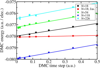
Figure 11: (Color online) DMC energy per electron against time step for a paramagnetic 3D HEG of density parameter $r_{s}=4$ a.u. at various system sizes $N$. A Slater wave function was used, except for the one curve labeled “Jas,” in which a Slater-Jastrow wave function was used. Twist averaging was not applied.

For any given system, the DMC population-control bias should fall off roughly as $N_{C}^{-1}$, where $N_{C}$ is the target population,umrigar_1993 so we have plotted the DMC energy against $N_{C}^{-1}$ in Fig. 12. Unlike time-step bias, population-control bias grows with system size. However, the increase in the bias with system size is slow. Population-control bias is caused by the correlation of fluctuations in the local energy and the DMC branching factor.umrigar_1993 Fluctuations in the local energy increase as $N^{1/2}$. If the exponential branching factors can be approximated by the first two terms in the Taylor expansion of the exponential then fluctuations in the branching factor increase as $N^{1/2}$. So the population-control bias in the energy per particle is roughly independent of system size. However, the fluctuations in the exponential branching factor grow more rapidly than $N^{1/2}$ in large systems, causing the bias to increase. Improving the accuracy of the trial wave function reduces population-control bias, as can be seen in the upper panel of Fig. 12.

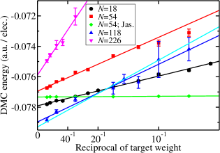
Figure 12: (Color online) Upper panel: DMC energy per electron against reciprocal of target population for a paramagnetic 3D HEG of density parameter $r_{s}=4$ a.u. at various system sizes $N$. Lower panel: gradient of the population-control bias (derivative of the DMC energy per electron with respect to the reciprocal of the target population) against system size. The DMC time step was 0.03 a.u., and a Slater wave function was used, except for the one curve in the top panel labeled “Jas,” in which a Slater-Jastrow wave function was used. Twist averaging was not applied.

X Conclusions

We have carried out a detailed study of finite-size effects in QMC calculations and have described a number of approaches for reducing or correcting them. Twist averaging greatly reduces the magnitude of single-particle finite-size errors, although residual single-particle errors due to the wrong shape of the CE twist-averaged Fermi surface are still significant in studies of the HEG. One can calculate these errors within HF theory, and hence correct for them.

Finite-size effects in the XC energy should be eliminated, either by adding a correction to the Ewald energy or by using the MPC interaction to calculate the final energies (although the Ewald interaction should be used to generate the configuration distribution, since the MPC interaction distorts the XC hole in finite systems). Finite-size corrections must also be applied to the KE. For HEGs, where analytic expressions for the low-$k$ behavior of the two-body Jastrow factor are available, we have found that it is important to include both the leading- and next-to-leading-order KE corrections at intermediate and high densities. The resulting QMC energy data are almost independent of particle number at typical system sizes. For real systems we recommend fitting the QMC-optimized Jastrow factor to Eq. (51) at small $k$, then using Eq. (55) to compute the correction to the KE.

Within HF theory the long-ranged nature of the exchange hole leads to additional errors in the exchange energy. These errors are absent in QMC calculations. They can also be viewed as arising from the nonanalytic behavior of the HF structure factor at ${\bf k}={\bf 0}$. We have constructed an accurate correction for these errors in HF theory.

For 2D systems the leading-order finite-size errors (using both the Ewald and MPC interactions) are caused by the slow convergence of the XC hole and the neglect of long-ranged correlations in the KE. The errors in the energy per particle scale as $O(N^{-5/4})$, suggesting that this form should be assumed in the extrapolation to infinite system size.

If the single-particle finite-size error is to be removed by extrapolation rather than twist averaging then the HF exchange energy should not be included in the extrapolation; just the KE. Furthermore, an estimate of the effective mass should be included in the extrapolation.

Tests at realistic system sizes show that time-step bias in DMC results does not get significantly worse as the system size is increased. Population control bias does get worse, but only slowly.

XI Acknowledgments

Financial support has been provided by Jesus College, Cambridge, and the Engineering and Physical Sciences Research Council (EPSRC), UK. Computing resources have been provided by the Cambridge High Performance Computing Service, the Imperial College High Performance Computing Service, and the UK National HPCx service. We thank D. M. Ceperley and M. Holzmann for helpful conversations.

Appendix A Finite-size errors in HF theory

For the 3D HEG, the HF exchange hole isgiuliani

$$\rho_{\rm x}(r) = -\frac{1}{N\Omega}\sum_{\sigma}N_{\sigma}^{2}\left|3\frac{\sin(k_{{\rm F}\sigma}r)-k_{{\rm F}\sigma}r\cos(k_{{\rm F}\sigma}r)}{(k_{{\rm F}\sigma}r)^{3}}\right|^{2}$$ (71)

$$\simeq -\frac{9}{2N\Omega r^{4}}\left(\frac{\Omega}{6\pi^{2}}\right)^{4/3}\sum_{\sigma}N_{\sigma}^{2/3},$$

where in the last line we have retained only the dominant nonoscillatory term at large separation, $k_{{\rm F}\sigma}=\left(6\pi^{2}N_{\sigma}/\Omega\right)^{1/3}$ is the Fermi wave vector for particles of spin $\sigma$, and $N_{\sigma}$ is the number of particles of spin $\sigma$. The hole has a slowly decaying tail that falls off as $1/r^{4}$, so there is a missing contribution to the exchange energy in a finite simulation cell. The interaction of each electron with its exchange hole should be $1/r$ (as enforced inside the simulation cell when the MPC interaction is used). So the missing contribution to the HF interaction energy is approximately

$$\Delta V_{\rm HF}^{\rm(1)} = \frac{N}{2}\int_{R_{\Omega}}^{\infty}\frac{4\pi r^{2}\rho_{\rm x}(r)}{r}\,dr$$ (72)

$$= -\frac{1}{2\pi r_{s}}\left(\frac{3}{4\pi N}\right)^{1/3}\sum_{\sigma}N_{\sigma}^{2/3},$$

where $R_{\Omega}$ is the radius of a sphere of volume $\Omega$. This gives a finite-size error in the HF energy per particle that falls off slowly as $N^{-2/3}$. This error will also be present in the Ewald energy. In addition to this missing contribution, there are errors arising from the fact that the part of the exchange hole that would lie outside the simulation cell if the system were infinite is distorted by being compressed back into the simulation cell to satisfy the sum rule. The charge of the missing tail is approximately

$$Q=\int_{R_{\Omega}}^{\infty}4\pi r^{2}\rho_{\rm x}(r)\,dr=\frac{-3}{N\pi}\left(\frac{\Omega}{6\pi^{2}}\right)^{1/3}\sum_{\sigma}N_{\sigma}^{2/3}\frac{1}{R_{\Omega}}=\frac{-3}{N\pi}\left(\frac{2}{9\pi}\right)^{1/3}\sum_{\sigma}N_{\sigma}^{2/3}.$$ (73)

If we assume that this missing charge is uniformly distributed inside a sphere of radius $R_{\Omega}$, we must subtract its unwanted contribution to the exchange energy, giving another correction

$$\Delta V_{\rm HF}^{\rm(2)}=-\frac{3NQ}{4R_{\Omega}}=\frac{3}{2\pi r_{s}}\left(\frac{3}{4\pi N}\right)^{1/3}\sum_{\sigma}N_{\sigma}^{2/3}.$$ (74)

(Other approximations, such as assuming $Q$ to increase linearly within $R_{\Omega}$ may be more accurate.) The total correction to the exchange energy (either Ewald or MPC) obtained within this real-space procedure is

$$\Delta V_{\rm HF}=\Delta V_{\rm HF}^{\rm(1)}+\Delta V_{\rm HF}^{\rm(2)}=\frac{1}{\pi r_{s}}\left(\frac{3}{4\pi N}\right)^{1/3}\sum_{\sigma}N_{\sigma}^{2/3}.$$ (75)

The result of applying this correction to the HF Ewald exchange energy is shown in Fig. 6, along with the result of applying the correction of Eq. (41). Both work well, although the correction of Eq. (41) is better.

Appendix B Equivalence of the MPC and XC correction

Consider a system of cubic symmetry. The difference between the MPC and Ewald XC energies is:

$$\langle\hat{V}_{\rm MPC}\rangle-\langle\hat{V}_{\rm Ew}\rangle = \frac{N}{2}\int_{\Omega}\rho_{\rm xc}({\bf r})\left(\frac{1}{r}-[v_{E}({\bf r})-v_{M}]\right)\,d{\bf r}$$ (76)

$$= \frac{N}{2}\int_{\Omega}\rho_{\rm xc}({\bf r})\left(\frac{2\pi}{3\Omega}r^{2}+\ldots\right)\,d{\bf r},$$

were we have used the expansion of the Ewald interaction from Eq. (19). Assuming that $\rho_{\rm xc}({\bf r})$ is well localized within the simulation cell, we can replace $\rho_{\rm xc}({\bf r})$ by $S_{\rm loc}({\bf r})-\delta({\bf r})$ and extend the range of integration to infinity to obtain

$$\langle\hat{V}_{\rm MPC}\rangle-\langle\hat{V}_{\rm Ew}\rangle = \frac{N\pi}{3\Omega}\int_{r<\infty}r^{2}S_{\rm loc}({\bf r})\,d{\bf r}$$ (77)

$$= -\frac{N\pi}{3\Omega}\left.\nabla_{\bf k}^{2}S_{\rm loc}({\bf k})\right|_{{\bf k}={\bf 0}}.$$

Since $S({\bf k})=\eta k^{2}+O(k^{4})$ in a cubic system, this reproduces Eq. (25):

$$\langle\hat{V}_{\rm MPC}\rangle-\langle\hat{V}_{\rm Ew}\rangle=\frac{2\pi N\eta}{\Omega}+\ldots.$$ (78)

The use of the first-order $\Delta V_{\rm Ew}$ correction may therefore be regarded as a first-order approximation to the MPC, in which the leading term in the small-$r$ expansion of the difference between $1/r$ and $v_{E}({\bf r})-v_{M}$ is taken into account but higher order terms are neglected.

References

- (1) S. Chiesa, D. M. Ceperley, R. M. Martin, and M. Holzmann, Phys. Rev. Lett. 97, 076404 (2006).
- (2) L. M. Fraser, W. M. C. Foulkes, G. Rajagopal, R. J. Needs, S. D. Kenny, and A. J. Williamson, Phys. Rev. B 53, 1814 (1996).
- (3) P. R. C. Kent, R. Q. Hood, A. J. Williamson, R. J. Needs, W. M. C. Foulkes, and G. Rajagopal, Phys. Rev. B 59, 1917 (1999).
- (4) A. J. Williamson, G. Rajagopal, R. J. Needs, L. M. Fraser, W. M. C. Foulkes, Y. Wang, and M.-Y. Chou, Phys. Rev. B 55, R4851 (1997).
- (5) W. M. C. Foulkes, L. Mitas, R. J. Needs, and G. Rajagopal, Rev. Mod. Phys. 73, 33 (2001).
- (6) C. Lin, F. H. Zong, and D. M. Ceperley, Phys. Rev. E 64, 016702 (2001).
- (7) R. Gaudoin and J. M. Pitarke, Phys. Rev. B 75, 155105 (2007).
- (8) R. J. Needs, M. D. Towler, N. D. Drummond, and P. López Ríos, casino version 2.1 User Manual, University of Cambridge, Cambridge (2007).
- (9) G. Rajagopal, R. J. Needs, S. Kenny, W. M. C. Foulkes, and A. James, Phys. Rev. Lett. 73, 1959 (1994).
- (10) G. Rajagopal, R. J. Needs, A. James, S. D. Kenny, and W. M. C. Foulkes, Phys. Rev. B 51, 10591 (1995).
- (11) A. Baldereschi, Phys. Rev. B 7, 5212 (1973).
- (12) P. P. Ewald, Ann. Phys. 64, 253 (1921).
- (13) The following Fourier series and transform conventions are used throughout this work: , ; , and .
- (14) B. Wood, W. M. C. Foulkes, M. D. Towler, and N. D. Drummond, J. Phys.: Condens. Matter 16, 891 (2004).
- (15) Note that the definition of the XC energy given here (the interaction of each electron with its XC hole) differs from the definition of the XC energy given in some other contexts (the difference of the energy within Hartree theory and the ground-state energy).
- (16) P. Gori-Giorgi and J. P. Perdew, Phys. Rev. B 66, 165118 (2002).
- (17) G. F. Giuliani and G. Vignale, Quantum theory of the electron liquid, Cambridge University Press (2005).
- (18) M. Allen and D. Tildesley, Computer simulation of liquids, Oxford Science (1990).
- (19) R. Maezono, M. D. Towler, Y. Lee, and R. J. Needs, Phys. Rev. B 68, 165103 (2003).
- (20) Y. Wang and J. P. Perdew, Phys. Rev. B 44, 13298 (1991).
- (21) D. Pines and P. Nozières, Theory of Quantum Liquids (Benjamin, New York, 1966).
- (22) Note that, in general, the average of the SF over a shell of symmetry-equivalent vectors is not the same as the spherical average of the SF evaluated at radius .
- (23) . Note that the periodicity of as a function of allows the volume of integration to be translated arbitrarily.
- (24) The Poisson summation formula (in 3D) states that for any smooth and rapidly decaying function .
- (25) If includes an term then the error in the XC-corrected Ewald energy falls off as .
- (26) A. Malatesta, S. Fahy, and G. B. Bachelet, Phys. Rev. B 56, 12201 (1997).
- (27) R. Gaudoin, M. Nekovee, W. M. C. Foulkes, R. J. Needs, and G. Rajagopal, Phys. Rev. B 63, 115115 (2001).
- (28) B. Wood and W. M. C. Foulkes, J. Phys.: Condens. Matter 18, 2305 (2006).
- (29) D. Bohm and D. Pines, Phys. Rev. 92, 609 (1953).
- (30) H. Kwee, S. Zhang, and H. Krakauer, Phys. Rev. Lett. 100, 126404 2008.
- (31) H. J. Monkhorst and J. D. Pack, Phys. Rev. B 13, 5188 (1976).
- (32) To evaluate the difference between the integral and sum of , we performed the integral analytically and computed the sum numerically. We reduced the parameter in until the difference converged to the reported precision.
- (33) T. Gaskell, Proc. Phys. Soc. 77, 1182 (1961).
- (34) The correction for the residual single-particle finite-size error from HF theory should be divided by the effective electron mass. This can be estimated as the ratio of the HF KE to the QMC KE. However, since the residual single-particle error is already a small correction, it makes little difference to the final results if one assumes an effective mass of 1 a.u.
- (35) N. D. Drummond, M. D. Towler, and R. J. Needs, Phys. Rev. B 70, 235119 (2004).
- (36) C. J. Umrigar, K. G. Wilson, and J. W. Wilkins, Phys. Rev. Lett. 60, 1719 (1988).
- (37) N. D. Drummond and R. J. Needs, Phys. Rev. B 72, 085124 (2005).
- (38) C. J. Umrigar, J. Toulouse, C. Filippi, S. Sorella, and R. G. Hennig, Phys. Rev. Lett. 98, 110201 (2007).
- (39) T. Kato, Commun. Pure Appl. Math. 10, 151 (1957); R. T. Pack and W. B. Brown, J. Chem. Phys. 45, 556 (1966).
- (40) P. Gori-Giorgi, S. Moroni, and G. B. Bachelet, Phys. Rev. B 70, 115102 (2004).
- (41) Note that in a 2D system corresponds to a point charge at the origin surrounded by a disk of negative charge. This has a significant quadrupole moment, irrespective of the symmetry of the system.
- (42) B. Tanatar and D. M. Ceperley, Phys. Rev. B 39, 5005 (1989).
- (43) P. López Ríos, A. Ma, N. D. Drummond, M. D. Towler, and R. J. Needs, Phys. Rev. E 74, 066701 (2006).
- (44) D. M. Ceperley, Phys. Rev. B 18, 3126 (1978).
- (45) D. M. Ceperley and B. J. Alder, Phys. Rev. Lett. 45, 566 (1980).
- (46) G. Ortiz and P. Ballone, Phys. Rev. B 50, 1391 (1994); G. Ortiz, M. Harris, and P. Ballone, Phys. Rev. Lett. 82, 5317 (1999).
- (47) C. J. Umrigar, M. P. Nightingale, and K. J. Runge, J. Chem. Phys. 99, 2865 (1993).