A scheme for fast exploratory simulation of azimuthal asymmetries in Drell-Yan experiments at intermediate energies. The DY_AB Monte Carlo event generator.

Abstract

In this note I report and discuss the physical scheme and the main approximations used by the event generator code DY_AB. This Monte Carlo code is aimed at preliminary simulation, during the stage of apparatus planning, of Drell-Yan events characterized by azimuthal asymmetries, in experiments with moderate center of mass energy $\sqrt{s}$ $<<$ 100 GeV.

1 Introduction

Here I discuss the general (physical) scheme of the series of event generators DY_AB, concentrating specifically on the last version of this code DY_AB5.

The event generator DY_AB5 is a generator of dilepton Drell-Yan events[1] in hadron-hadron, hadron-nucleus and hadron-(partly polarized molecular target) collisions. It is aimed at fast preliminary simulation of that subset of Drell-Yan experiments, where

(i) the center of mass energy is “intermediate” (from a few to some tenths GeV);

(ii) the projectile may be any light hadronic species (charged pion, proton, antiproton), possibly polarized;

(iii) the target is in general a molecular species, with partial normal polarization of some of its component nuclei;

(iv) the final leptons present azimuthal asymmetries and these asymmetries are the goal of the measurement.

Several experimental proposals have been presented or are in preparation in this field[2, 3, 4, 5, 6].

The main difficulty of such experiments is the need to select regions of the overall phase space where the event rates are small (in particular: transverse momentum over 2 GeV/c), and where two event numbers (e.g.: before/after reversing spin) must be compared to identify small asymmetries. It is essential to understand from the very beginning which overall event numbers are needed to reach a satisfactory population of the interesting subregions.

The here discussed code is aimed at such “preliminary” investigations, for experimental planning only. Since it is based on strong phenomenological components, it is not suitable as it is for theoretical analysis at quark-parton level.

Up to date, five (private) versions of this code, named DY_AB1, 2, 3, 4, and 5, have been used and tested by the author and by other users both for phenomenological publications[7, 8, 9, 10, 14, 11] and for exploratory simulations aimed at experimental proposals[2, 3, 5] (see e.g. [12], [13]).

The latest release DY_AB5 is public.

This code is not a multi-purpose code. Its main advantages are in its specificity, and are: (i) easy insertion of new parametrizations for distribution functions associated with azimuthal asymmetries, (ii) easy control and modification of the code, (iii) possibility of simultaneous treatment of events in the Collins-Soper reference frame and in the fixed target or collider frame, (iv) fast generation of events, (v) satisfactory phenomenological reproduction of transverse momentum distributions.

The present note is not the “readme” handbook of the code. The code itself is normally accompanied by a readme file supplying user help. Here I discuss the physical scheme used for the event generation. This is inspired by the parton model, but some simplifications or phenomenological parameterizations have been introduced into the standard relations for the cross section.

The reasons behind these simplifications are two:

(i) This code is not aimed at improving the theoretical understanding of quark-quark interactions; it is used for reproducing as realistic as possible event distributions and associated errors, in measures where some gross features of the data are already well known, while other ones are largely unknown.

(ii) At the present stage, the real point is to understand whether or not certain measurements will be possible, or at which extent they will be possible. This requires a huge amount of exploratory simulations, to be run in the smallest possible time and with the maximum possible flexibility.

I hope this presentation clarifies in which frameworks the code can be used, or should not be used.

1.1 Development notes

This code has been written in c++ since the first version. It began as a toy model Drell-Yan generator, aimed at fast exploratory simulation for the Drell-Yan measurement within the PANDA experiment[12]. After the very first applications, the number of options has increased exponentially.

It was initially used by people of some experimental collaborations, in a form that permitted them to handle input in a simple way, assuming that they would not need touching the code. This has shown to be unrealistic. On the other side, unrealistic as well has been the hope that people could be made able to modify the code themselves, without interacting at all with the author. And also attempts to organize a “once and for all” form of the code have failed, just for the fact that the field is quickly evolving. For example, it is difficult to find a “universal” form for the new distribution functions that one could like to insert in the next five years.

So, the general idea is that apart for a central core of classes/functions there is nothing sacred in the code structure, and that users should be able to modify the code via an as small as possible interaction with the author.

The first versions like DY_AB1 fully exploited the possibility of writing complex hierarchies, offered by c++. In DY_AB4 this structured form was abandoned, but for efficiency purposes massive use was made of pointers. DY_AB4 is well tested, and is the most efficient code of this series. A short presentation of this code may be found in [12]. Its main disadvantage was hard readability, since to increase efficiency it exploited systematically the fortran-style technique of organizing big data structures, with functions working on these data without explicitly getting them as arguments (the “common” areas in fortran; in c++ the same is obtained via pointers to data classes). The absence of explicit arguments in the function calls makes the code hierarchy difficult to see at first reading.

DY_AB5 is less efficient (about 30 % more time-consuming). The advantage is that it is much easier to read and modify (pointers have mostly disappeared). It offers more pre-cooked options as far as unpolarized and single-polarization Drell-Yan are concerned.

2 General theoretical notes

2.1 General scheme

This code typical cycle consists of the following steps:

1) Random event generation in the Collins-Soper frame for a specified class of projectile and of target hadrons (e.g. negative pion and polarized proton).

2) Transformation of these events first to the hadronic center of mass frame (“collider frame”), and next to the fixed target frame.

3) Loop over events taking into account the composition of the (molecular) target in terms of different nuclei.

4) If required, a number of repetitions of a multi-event simulation is performed, possibly with spin reversal.

5) If required, statistical analysis of azimuthal asymmetries is performed, calculating averages and fluctuations of the results obtained in the simulations of step (4).

Here I discuss the general problems and some implementation detail connected with steps (1) and (2).

The exact and complete cross sections on which the event generation is based may be found in [14]. There, two simulation schemes are compared. DY_AB5 is based on what is named “scheme II” in ref.[14]. An alternative code has been prepared by this author, based on “scheme I”, and in [14] the differences in the outcome are shown. Also, the reasons are discussed why “scheme I” is more proper and supposed to take over in the long run, but not yet well suited given the present state of the art on the phenomenology side.

Formulas reported in [14] and implemented in DY_AB5 are rather long. Here, a simplified version of these relations is discussed, to clarify the general cross section form, the main approximations contained in it, and the way the code exploits it.

In the language of [14] “Scheme I” is the parton model cross section for Drell-Yan events with most of the necessary details: several products of distribution functions associated with unpolarized and polarized partons and hadrons, and with all quark and antiquark flavors, are summed .

“Scheme II” exploits some more approximations: (i) A cumulative event distribution is factorized out of the sum of all terms. This distribution is built by a set of simplified parton distribution functions $f$, and is phenomenological in the transverse momentum dependence. (ii) Generalizing an approximation method that may be found e.g. in[15] all the least known distribution functions $h$ (those associated with azimuthal asymmetries) are expressed as ratios $h/f$. (iii) Each such $h/f$ term is added to the sum, “valence-weighted” by ratios like 4/9 etc.

2.2 The overall cross section

The relations discussed in the following may be found, e.g., in [17] and [18]. The problem is that in these two works several of such relations assume systematically different forms. Since this difference is present in all the relevant literature, we name these two works “ref.A” and “ref.B” and systematically report the differences.

I name “mass” $M$ the invariant mass of the lepton pair (it is also named $Q$ in some references). The indexes “1” and “2” represent the target and beam hadrons.

The Drell-Yan differential cross section can be written in an approximate factorized way, inspired by the parton model (see [16], chapter 5, and refs.A and B):

$${d\sigma\over{d\tau dX_{F}dP_{t}d\Omega}}\ =\ {K(\tau)\over s}\cdot\bar{S}(\tau,X_{F})\cdot S^{\prime}(P_{t})\cdot A(\theta,\phi,\phi_{s}).$$ (1)

or equivalently in the form

$${d\sigma\over{dX_{1}dX_{2}dP_{t}d\Omega}}\ =\ {K(\tau)\over s}\cdot S(X_{1},X_{2})\cdot S^{\prime}(P_{t})\cdot A(\theta,\phi,\phi_{s}).$$ (2)

As customary, $s$ is the squared invariant mass of the two colliding hadrons.

$$s\ \equiv\ (E_{CM})^{2}\ =\ 2m_{p}(m_{p}+E_{\bar{p},LAB}).$$ (3)

The scaling assumption means that the only dependence of eq(1) or (2) on $s$ should be contained in the $1/s$ term.

$X_{F}$ and $\tau$ are invariant adimensional variables associated with the beam-axis momentum projection, and with the virtuality, of the virtual photon produced in $\bar{p}$ $+$ $p$ $\rightarrow$ $X$ $+$ $\gamma^{*}$ $\rightarrow$ $X$ $+$ $\mu^{+}\mu^{-}$. The pair $\tau$, $X_{F}$ can be substituted by the equivalent pair $X_{1}$, $X_{2}$. Then $\bar{S}$ and $S$ are related by a Jacobian factor. The definition of $\tau$, $X_{F}$, $X_{1}$ and $X_{2}$ is given below, where it requires some discussion.

$\vec{P}_{t}$ is the transverse $2-$dimensional component of the 4-momentum of the virtual photon, with respect to the beam axis. (it is also named $q_{t}$, or $Q_{t}$).

The angular variables $\theta$, $\phi$, $\phi_{s}$ appearing in $A(\theta,\phi,\phi_{s})$ are measured in a reference frame where the virtual photon is at rest. In this frame $\theta$ and $\phi$ are the polar and azimuthal angles of the momentum of one of the two muons, while $\phi_{s}$ is the azimuthal angle of the target spin. These variables are discussed later, in the paragraph on the angular distributions.

In the right hand sides of equations (1) and (2) $\bar{S}(...)$ and $S(...)$ differ because of the direct substitution $\tau$ $=$ $\tau(X_{1},X_{2})$, $X_{F}$ $=$ $X_{F}(X_{1},X_{2})$, and because $\bar{S}(...)$ $=$ $JS(...)$, where $J$ is the Jacobian of the coordinate transformation between $d\tau dX_{F}$ and $dX_{1}dX_{2}$.

The coefficient $K$ $=$ $K(\tau)$ is normally named “K-factor” and is predicted to be 1 in the parton model. Actually it is neither 1 nor constant (it is $\approx$ 2). Traditionally $K$ contains all the parton model violations, which are so kept apart from the rest of the cross section. Summarizing the PQCD corrections into a single $\tau-$depending factor is at a certain extent justified for $\tau$ far from its kinematic boundaries 0 and 1 (see [16], subsections 5.2, 5.3, 5.5, and [19]), and for moderate transverse momenta $<<$ M. At these conditions the parton-parton $\rightarrow$ $\gamma^{*}+X$ cross section is dominated by those terms where $X$ subtracts no invariant mass from the parton-parton $\rightarrow$ $\gamma^{*}$ transition predicted in the plain parton model.

The above cross section factorization is formally exact within the parton model, but in the above reported form it hides that $S^{\prime}(P_{t})$ is (weakly) dependent on $\tau$ and $X_{F}$, and that $A(\theta,\phi,\phi_{s})$ depends on $X_{1}$, $X_{2}$, $P_{t}$, $M$.

In the code these dependencies have been taken into account. The previous equations are however written in such a way to focus on the $assumed$ variable hierarchy that allows for a kinematic separation of the $S$, $S^{\prime}$ and $A$ contributions (see e.g. refs.A and B for examples of the experimental procedure to extract these terms from incomplete phase space):

(i) $S(X_{F},\tau)$ does not depend on $P_{t}$ and on the angular variables, so for any assigned $X_{F},\tau$ (or equivalently, $X_{1},X_{2}$) it can be calculated from the cross section integrated over all the $P_{t},\theta,\phi$ phase space and summed over spin;

(ii) $S^{\prime}(P_{t})$ $\equiv$ $S^{\prime}(X_{f},\tau,P_{t})$ does not depend on the angular variables, so it can be determined by $\theta,\phi$ integration plus a sum over spin.

The function $S^{\prime}(P_{t})$ and $A(\theta,\phi,\phi_{s})$ are defined so that

$$\int S^{\prime}(P_{t})\ =\ 1,\ \ \int A(\theta,\phi,\phi_{s})d\Omega_{\theta,\phi}\ =\ 1,$$ (4)

integrating over all the phase space, for any given $\phi_{s}$. So the total $\sigma$ is just the integral of $K(\tau)S(X_{1},X_{2})$.

2.3 The longitudinal term $S(X_{1},X_{2})$: definitions and dangerous ambiguities.

We can describe the meaning of $\tau$ and $X_{F}$ by the following relations:

$$\tau\ \equiv\ {M^{2}\over s}\approx\ {M^{2}\over M^{2}_{max}}$$ (5)

$$X_{F}\ \approx\ \Bigg{(}{P^{\gamma}_{z}\over{{P_{\gamma}}_{max}}}\Bigg{)}_{CM}$$ (6)

$\sqrt{\tau}$ is the ratio of the virtual photon virtuality $M^{2}$ to its kinematic maximum $s$, reached in an exclusive $\bar{p}p\rightarrow l^{+}l^{-}$ annihilation into dilepton. $X_{F}$ is approximately the ratio of the beam axis component of the virtual photon momentum (in the hadron collision CM) to its kinematic maximum. The precise definition of $X_{F}$ is not univoque in the literature, as discussed below. Whatever the exact definition, $X_{F}$ and $\tau$ are normally defined as $measurable$ scalar functions of the projectile and target four-momenta. Alternatively, they can be substituted by their combinations $X_{1}$, $X_{2}$, whose approximate meaning is the ratio of the longitudinal component of each of colliding quarks to the parent hadron momentum in the reaction CM:

$$X_{i}\ \approx\ \Bigg{(}{{(P_{z})_{quark}}\over{(P_{z})_{hadron}}}\Bigg{)}_{CM}.$$ (7)

For $X_{1}$ and $X_{2}$ several definitions can be found, all approximately equivalent at large $s$ and $M$. These definitions fall into two groups: (a) “theoretical” definitions, given in terms of the (unmeasured) light cone momenta of the colliding quarks; (b) “experimental” definitions (as in ref.A or B), which express $X_{1}$ and $X_{2}$ as combinations of the (measured) variables $\tau$ and $X_{F}$. In the “theoretical” case, $X_{i}$ is the ratio of the large light-cone component of the $i-$quark momentum to the corresponding component of the momentum of its parent hadron. For a rigorous theoretical definition of $X_{1}$ and $X_{2}$ see e.g. [20].

In the high energy limit experimental definitions are supposed to reproduce the corresponding theoretical ones, so to access approximately to the quark momenta. It must be remarked that this is $not$ the situation, in the some portions of the kinematic range considered here.

The definition of $\tau$ is the same in refs.A and B, and seemingly “$\tau$” means the same thing in all the literature on the subject:

$$\tau\ =\ M^{2}/s\ \ \ \ (refs.\ A\ and\ B)$$ (8)

On the contrary, for $X_{F}$, $X_{1}$, and $X_{2}$ we have non univoque definitions. Ref.A uses

$$X_{F}\ =\ {{2P_{L}}\over\sqrt{s}}\ \ \ \ (ref.\ A)$$ (9)

$$X_{F}\ =\ X_{1}-X_{2},\ \ \ \tau\ =\ X_{1}X_{2}\ \ \ (ref.\ A).$$ (10)

Ref.B uses

$$X_{F}\ =\ {{2P_{L}}\over{\sqrt{s}(1-\tau)}}\ \ \ \ (ref.\ B)$$ (11)

$$X_{F}\ =\ (X_{1}-X_{2})/(1-\tau),\ \ \tau\ =\ X_{1}X_{2}\ \ (ref.\ B).$$ (12)

The definitions of ref.A are easier to use and more common in the literature, so the code sticks to them. With them it is necessary to take care with the kinematic limits: $|X_{F}|_{max}$ $<$ 1.

When comparing differential cross sections referred to the variables $X_{1},X_{2}$ or $X_{F},\tau$, jacobian conversion factors are necessary.

The differential cross sections of equations (1) and (2) enjoy complete scaling properties for the $\bar{p}p$ case, while in the $\pi p$ case a mass-dependent[21] term is introduced by ref.A, it is important for large $X_{\pi}$ and considered in the code.

Full scaling means that $(P_{t},\theta,\phi)-$integrated cross sections only depend on the $X-$set variables, apart for an $s$ dependence confined to the $1/s$ term. Compared data of ref.A (250 GeV/c beam energy) and ref.B (125 GeV/c) on $\pi-p$ DY scattering show approximate scaling.

$K$ is assumed to be a function of $\tau$ in ref.A (and in the code), while most experiments (see the DY database from[22]) use it as a constant normally $\approx$ 2. For large $\tau$ values, the data by ref.A show that this dependence is relevant, and the results of the calculation by [19] support this point. The largest part of the events concentrate at the lowest part of the involved $\tau-$range (wherever it begins), and this may make it difficult to scan a large $\tau-$range, to establish precise dependencies for $K$ on $\tau$.

As remarked in ref.B, the choice of the $K$ value depends on the choice of the normalization for the quark distribution functions, which is not univoque. Ref.B reports a detailed and systematic discussion of the different normalization methods and of the consequent changes in the values of the distribution function parameters and of $K$. This can be exploited, with the warning of using distribution functions according to the notations of ref.B (see below).

In the default version of the code DY_AB5, $S(\tau,X_{F})$ has been reconstructed using the parameterized form given in appendix A of ref.A, together with the kinematic definitions and structure functions contained in the main text of ref.A.

This allowed me to fit $\pi^{-}-$Tungsten DY differential cross sections reported by that experiment at 252 GeV/c.

When notations of the two works are conformed each other, the distribution functions fitted from ref.A allow to reproduce reasonably $\pi^{-}-$data reported by ref.B at 125 GeV/c. To reproduce the $\bar{p}-A$ DY data of the same experiment, proton quark distribution functions must be used as antiproton antiquark distribution functions, and then the reproduction is reasonable.

In both references and everywhere in the literature $S(X_{1},X_{2})$ has the form

$$S(X_{1},X_{2})\ =\ G(X_{1},X_{2})\Sigma_{i}\bar{F}(X_{1})F(X_{2})$$ (13)

where $G(X_{1},X_{2})$ is a kinematic factor proportional to $(1/X_{1}X_{2})^{2}$ (ref.A) and $1/X_{1}X_{2}$ (ref.B). In general its exact form depends on notations and changes from paper to paper. The exponent “1” or “2” in the $1/X_{1}X_{2}$ factor is very important because it indicates whether the distribution functions $F(X)$ must be read as $F(X)$ or as $XF(X)$ (see below).

$\bar{F}$ and $F$ are linear combinations of the $\bar{q}/q$ main distribution functions $u(X)$, $d(X)$, $s(X)$. For these we have

$$X\cdot u(X)_{A}\ =u(X)_{B},\ \ X\cdot d(X)_{A}\ =d(X)_{B},\ etc.$$ (14)

So, e.g., the normalization $\int XdX(u+d)$ $=$ 0.34 in ref.A becomes $\int dX(u+d)$ $=$ 0.34 in ref.B. The $\alpha$ parameter appearing in the typical parameterization $u(X)$ $=$ $X^{\alpha}(1-X)^{\beta}$ changes by one unit passing from ref.A to ref.B, and so on.

The important remark is that this ambiguity $q(X)$ $\leftrightarrow$ $Xq(X)$ is present throughout all the literature on the subject, not only in these works. This is a very delicate point and must be taken into account whenever new terms are added to the code.

2.4 The $P_{t}$ dependent $S^{\prime}(P_{t})$.

The traditional parton model literature is built on the collinear approximation. So, for the $P_{t}-$dependent parts one must rely on phenomenological fits.

Experiments A and B did not impose a low-$P_{t}$ cutoff, with the consequence that their small $P_{t}$ data show a completely different qualitative behavior. Measured values of the function $S^{\prime}(P_{t})$ can be seen e.g. in ref.A figs.23 and 25 ($\pi+p$ case), or in ref.B fig.9 ($\pi+p$ and $\bar{p}+p$ cases). Since azimuthal asymmetries are very small for $P_{t}$ $<$ 1 GeV/c, this difference is not relevant for the purposes of planning experiments on azimuthal asymmetries in Drell-Yan. For pions the default option is the distribution used in ref.A.

The code however offers a series of alternatives. The class that handles all $P_{t}$-distributions is PT2. The use of a specific distribution requires subclassing.

Some options are already present in the code DY_AB5:

PT2_Old : public PT2 is further subclassed into three possibilities:

(1) The distribution by Conway et al[17] to reproduce $\pi^{-}-$tungsten at 250 GeV/c.

(2) The one by J.Webb[23] (E866 collaboration) for proton-nucleus at 800 GeV/c. hep-ex/0301031

(3) The one by Chang[24] (E866 collaboration) for the same measurement of J.Webb at the $J/\psi$ mass.

(4) The class PT2_Simple_Asym : public PT2 of the form $NP_{t}^{n}/(P_{t}^{2}+P_{o}^{2})^{m}$. This shape is useful for the azimuthal asymmetry terms (see below).

The most relevant features of the measured $S^{\prime}(P_{t})$ are (i) a not too strong dependence on $X_{1},X_{2},s$, (ii) for $P_{t}$ $<$ 2 GeV/c the distribution is not steeply decreasing (in case ref.A it is increasing up to 0.5 GeV/c); For $P_{t}$ $>$ 2 GeV/c it decreases steeply (but with power law, not exponential); (iii) the average $P_{t}$ is near 1 GeV/c, and as well known (see e.g. [16]) it is larger than in lepton-induced DIS and in hadron-hadron semi-inclusive meson production.

In the preliminary simulation of a Drell-Yan experiment on azimuthal asymmetries, a good phenomenological shape of $S^{\prime}(P_{t})$ is a key success factor, because measured and/or predicted leading-twist azimuthal asymmetries do increase at increasing $P_{t}$, obliging the experiment to select events at a as large as possible $P_{t}$. However, due to the very fast decrease of $S^{\prime}(P_{t})$ for $P_{t}$ $>$ 2 GeV/c, the choice of a too large $P_{t}$ cut-off can make a measurement prohibitive because of fast falloff of the event rates at large $P_{t}$.

Ref.A reports an explicit parameterization for $S^{\prime}(P_{t})$ (relative to $\pi-$induced Drell-Yan). Ref.B reports data and some models for the $P_{t}$ distributions in both $\bar{p}p$ and in $\pi p$ DY. In the region $P_{t}$ $>$ 3 GeV/c error bars are too big to draw any conclusion, but for $P_{t}$ up to 3 GeV/c $\pi p$ and $\bar{p}p$ $P_{t}-$distributions are very similar.

For pion and antiproton projectiles I did not modify the parameterization inherited from appendix A (pion) of ref.A and from ref.B ($\bar{p}$). The pion one is $not$ scale-independent. It depends explicitly on $M$ $=$ $s\tau$, and produces a slow increase of the average $<P_{t}^{2}>$ at increasing $s$ and constant $\tau$.

For proton projectiles, the parameterization by J.Webb[23] is probably more recommendable.

2.5 Isospin/flavor composition.

Up to a few years ago the models on the functions associated with azimuthal asymmetries didn’t go to such details like the $Z/A$ composition of the target. For this reason, the first code DY_AB1 did not care isospin/flavor matters. After Hermes and Compass results, some flavor and isospin-dependent parameterizations for single-spin asymmetries have appeared (see e.g.[9, 25, 26, 27]), obliging the codes since DY_AB2 onwards to take these problems into account.

On the experimental side the Z/A composition is important for another reason: it determines the effective dilution factor of the target polarization.

DY_AB5 takes into account events coming from separate pieces of a molecular target, taking the individual dilution factor of each nucleon into account. So to reproduce a $NH_{3}$ target with 85 % polarized $H$, one may arrange code parameters so to require about 4 events on an unpolarized proton or neutron and one event on a polarized proton. After this, any specific sorted event, e.g. $\pi_{-}-$neutron, will actually need to be translated into a $\bar{u}u$, a $\bar{d}d$ or a $\bar{s}s$ event.

In DY_AB5 this is taken into account by $X-$averaged weighting factors. The criterion and the weights for the relevant cases are discussed in detail in ref.[14]. There, also the errors associated with this technique are shown, in “approximate vs exact” scatter plots.

The point is that a sum of the kind

$$\sum_{flavor}\Big{(}S_{leading}[1+S_{asymmetry}/S_{leading}]\Big{)}$$ (15)

where each term is flavor-specific, is approximated in the form

$$S_{leading}\Big{(}1+\sum_{flavor}W_{flavor}[S_{asymmetry}/S_{leading}]\Big{)},$$ (16)

where the leading term is common, the weights are constant (and of course depend on the projectile-target hadron pair for the sorted event), the terms $[...]$ are flavor-specific functions where it is not possible to separate the numerator from the denominator.

Weight factors are needed to compensate the fact that e.g. the asymmetries associated with $\bar{d}d$ collisions have scarce relevance in a process like $\bar{p}p$ or $\pi_{-}p$, while they have more in $\pi_{+}n$. As observed in [14], the discrepancies between the “exact” scheme and the constant-weight scheme are relevant when both the colliding hadrons have small $X$.

In practice, planned experiments will try to stay as far as possible from this region, since common belief is that transverse spin effects are small there. In addition, although it would be better to sort events according to the former scheme, phenomenological parameterizations do normally extract the ratios $[S_{asymmetry}/S_{leading}]$ according to the latter scheme. Paradoxically, as remarked in [14], this makes the latter scheme more proper than the former for a simulation.

So, although the author of this note has prepared since long a “DY_AB6” code working according with a more exact scheme (the one used for the simulations of [14]), such a code is unlikely to be useful for still some time.

2.6 Angular distributions

Angles $\theta$, $\phi$ and $\phi_{s}$ in the function $A(\theta,\phi,\phi_{s})$ are measured in a reference frame with origin in the center of mass of the muon couple. In other words, the origin of this frame coincides with the virtual photon position. The axes of this frame can be oriented in several ways. One leads to the so-called Collins-Soper frame[28] (CS), with $\hat{z}$ axis parallel to the difference of the momenta of the projectile and of the target $nucleon$. The transverse axes are oriented so that the $xz$ plane contains the virtual photon momentum. Other common alternatives put the $\hat{z}$ axis along the beam or target direction in the lepton CM.

The DY_AB5 code sorts events in the CS frame. This fact becomes relevant when events are transformed to the fixed target or to the collider frame (see related section below).

In the CS frame, $\theta$ and $\phi$ are the angles formed by $one$ of the muons ($\mu^{+}$ from now onwards), and $\phi_{s}$ is the target spin orientation.

For a $qualitative$ understanding of the kinematics for most (not all) events, one may imagine a virtual photon with transverse momentum not much larger than 1 GeV, and $|X_{F}|$ not too close to zero, so that the longitudinal momentum of the photon is larger than the transverse momentum. Then the CS $z$ axis is roughly parallel to the collider one. Also the CS $xy$ plane is roughly parallel to the collider $xy$ plane, but the CS $x$ and $y$ axes are randomly rotated by an angle $\phi_{coll}$ with respect to their collider configuration. This $\phi_{coll}$ is the angle between the $xy-$component of the virtual photon and the $x$ axis in the lab. The $x$ axis of the CS frame coincides physically with the transverse component of the virtual photon 3-momentum. Then the transverse proton spin, which is fixed along the $x$ axis in the collider frame, lies on the CS $xy$ plane with angle $\phi_{s}$ $=$ $-\phi_{coll}$.

These approximations are not used in the code, but can be useful to understand the meaning of the employed angles, and to have an idea of the distribution of useful events in a collider frame.

In the Collins-Soper frame the angles $\theta$ and $\phi$ are polar and azimuthal angles of the momentum of one of the two leptons and are randomly distributed. Also the spin angle $\phi_{s}$ is randomly distributed in the CS frame. In absence of information on two of these angles, the third one is homogeneously distributed over all of its phase space. However, altogether their distributions are correlated by $A(\theta,\phi,\phi_{s})$ in the cross section.

In the simulation events, are initially flat-sorted with respect to all the kinematic variables $X_{1}$, $X_{2}$, $P_{t}$, $\theta$, $\phi$, $\phi_{s}$. The sorted events are accepted/rejected according to the cross section expressed by eq.(1) where, at the level of single spin experiments,

$$A(\theta,\phi,\phi_{s})\ =\ 1\ +\ cos^{2}(\theta)\ +\ {{\nu(X_{1},X_{2},P_{t})}\over 2}sin^{2}(\theta)cos(2\phi)\ +\$$

$$+\ |\vec{S}_{2}|B(X_{1},X_{2},P_{t},M,\theta,\phi,\phi_{s})$$ (17)

The unpolarized asymmetry measured in ref.A is contained in the $\nu...$ term. Single spin asymmetries arise from the $|\vec{S}_{2}|B(...)$ term. Two origins for such terms have been considered here, corresponding to different origins for the azimuthal term.

The Sivers[29] asymmetry considers a term of the form

$$B=2{m_{p}\over M}sin(2\theta)sin(\phi-\phi_{s})H_{a}(X_{1},X_{2})$$ (18)

while the Boer-Mulders[15, 30] asymmetry is of the form

$$B=-{1\over 2}\sqrt{\nu\over\nu_{max}}sin^{2}(\theta)sin(\phi+\phi_{s})H_{b}(X_{1},X_{2})$$ (19)

Any of the above azimuthal asymmetries (unpolarized, Sivers, BMT) can be disentangled from the other two by a suitably weighted $\phi$ integration. The “statistical analysis” option of the code offers this possibility.

2.7 Parameterizations for the nonstandard distribution functions

As above written, the leading distribution functions are bypassed by assuming a phenomenological (correctly behaving and scaling in a wide range of kinematics) form for the “standard” event distribution, i.e. for the $(\theta,\phi)-$averaged part of the event distribution.

For the “nonstandard” terms (i.e. those ones that produce nontrivial angular distributions in the CS frame) the code includes as a first possibility some phenomenological parameterizations that have become recently available in the literature, and as a second option the possibility to chose freely the parameters for simple pre-determined shapes.

The functions associated with the nonstandard terms have been put in places where it is easy to find them (in the file c_dy_master.cpp). So, if one wants to change radically the shape of these functions it is possible to do it. The code has been written assuming that any potential user could be interested in adding supplementary terms to this set. In other words, I assume that in the next ten years there will be no special reasons to change the “standard” part of the cross section, while updates and news on the asymmetry side will be frequent.

Although it is possible to add new parameterizations, respecting some formats makes things easier. Here I would like to discuss these formats.

1) Let us write the $A$ term in eq.(17) in the most general form

$$A(......)\ \equiv\ 1\ +\ cos^{2}(\theta)\ +\ \sum\Big{(}F(X_{1},X_{2},P_{t})F^{\prime}(\theta)F^{\prime\prime}(\phi,\phi_{s})\Big{)}$$ (20)

It must be reminded that according with the scheme adopted in this code each $F$ term is the $ratio$ between a term associated with a given kind of angular asymmetry and the “standard” term, that carries with itself the $1+cos^{2}(\theta)$ angular dependence. Since most of the available parameterizations give directly such a ratio, this is the most convenient form, as earlier discussed in this work.

2) The code assumes factorization between longitudinal and transverse degrees of freedom, and between terms coming from projectile and target, in the functions terms $\nu$ and $B$ in eq.(17). These functions have the form

$$F(X_{1},X_{2},P_{t})\ \equiv\ f_{1}(X_{1})f_{2}(X_{2})f_{t}(P_{t}),$$ (21)

3) For the longitudinal components $f_{i}(X_{i})$ the code assumes the form

$$f_{i}(X)\ \equiv\ NX^{\alpha}(1-X)^{\beta}$$ (22)

To insert completely different functions is possible but it is of course much easier to change three parameters for any quark flavor.

4) The transverse term is

$$f_{t}(P_{t})\ =\ {{\int d^{2}k_{1}d^{2}k_{2}[g_{1}(\vec{k}_{1})g_{2}(k_{2})]_{asymmetry}\delta^{2}(\vec{P}_{t}-\vec{k}_{1}-\vec{k}_{2}).}\over{\int d^{2}k_{1}d^{2}k_{2}[g_{1}(\vec{k}_{1})g_{2}(k_{2})]_{standard}\delta^{2}(\vec{P}_{t}-\vec{k}_{1}-\vec{k}_{2}).}}$$ (23)

where as previously reminded, the numerator is the really asymmetric term, the denominator is the leading standard $P_{t}-$dependence.

5) For the transverse part it is responsibility of the user to introduce directly the convolution of the two transverse momentum distributions corresponding to the colliding partons. In other words, the code assumes that one directly introduces $f_{t}(P_{t})$ in eq.(20).

The last constraint is not a true constraint, since all the parameterizations known to me employ gaussian shapes, whose convolution may be easily computed in analytical way. On the other side, this means spared execution time for the code.

7) Frequently, the result of eq.(23) $f_{t}(P_{t})$ will assume the form that I name “$f_{simple}(P_{t})$”:

$$f_{simple}(P_{t})\ \equiv\ NP_{t}^{n}/(P_{t}^{2}+P_{o}^{2})^{m}.$$ (24)

Because of the common use of Gaussian distributions, this form for the ratio $f(P_{t})$ is quite common. So the code gives, among other options, this one.

To implement the calculated $P_{t}-$convolutions, or to insert phenomenological ones (including the “standard” term $S(P_{t})$ in eq.1) the code offers a class PT2 that may be subclassed two ways:

(i) Exploiting the class PT_Simple_Asym : public PT2 to directly insert the parameters $N$, $P_{o}$, $n$, $m$, into the form $NP_{t}^{n}/(P_{t}^{2}+P_{o}^{2})^{m}$.

(ii) Subclassing the class PT2 by another user-assumed distribution. As above discussed, the code itself offers several examples of this procedure, i.e. all the relevant alternatives offered for the $P_{t}$-dependence of the leading “standard” term.

The already present $default$ parameterizations correspond, for the Boer-Mulders effect, to the $x-$independent $\nu(k_{t})$ function given in [15], for the Sivers effect to the two alternatives [9, 25].

For the $k_{t}-$unintegrated Transversity distribution the default $(N,\alpha,\beta)$ parameters are $(1,0,0)$ and no predefined set was considered.

3 Interesting Plots

In the following, some collections of simulated Drell-Yan events are compared with the measured distributions, for negative pions on Tungsten. At the kinematics of interest for DY_AB5 the two experiments with far the best statistics in the mass range 4-9 GeV/c² are E615 at Fermilab and NA10 at CERN. The code DY_AB has been based on the scheme and parameters given by E615 in [17], however it works equivalently with NA10 data[31, 32], coming from nearby kinematic regions.

3.1 Comparison with experimental data: E615

To produce fig.1, DY_AB5 has sorted 100,000 Drell-Yan events for negative pions with beam energy 252 GeV on a Tungsten target, in the dilepton mass range 4-7 GeV/c². From this set, I extract the subset of events with $\sqrt{\tau}$ in the range 0.254-0.277 (mass from about 5.5 to 6 GeV/c²). The distribution of these events with respect to $x_{F}$ may be compared with the cross sections given in [17], table VI.

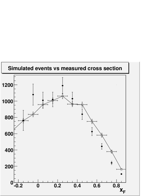
Figure 1: Filled squares: E615 data for $\sqrt{\tau}$ in the range 0.254-0.277. Empty squares with joining line: Simulation (see text).

Figure 2: Filled squares: E615 data (252 GeV pion beam) for $\sqrt{\tau}$ in the range 0.392-0.415. Empty squares with joining line: Simulation (see text).

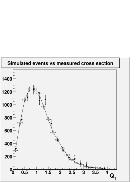
Figure 3: Filled squares: E615 data for $x_{F}$ in the range 0-0.1. Empty squares with joining line: Simulation (see text).

Figure 4: Filled squares: E615 data for $x_{F}$ in the range 0.6-0.7. Empty squares with joining line: Simulation (see text).

In fig.1 the empty squares joint by a line are the event numbers sorted by DY_AB5. Horizontal bars represent the size $\Delta x_{F}$ $=$ 0.1 of each bin, vertical bars the statistical error $\sqrt{N}$. The full black squares with no horizontal error bar are the numbers from table VI of [17], rescaled by a common constant factor so to transform cross section values into expected values for the bin populations.

Sets of data corresponding to smaller $\sqrt{\tau}$ cover a slightly smaller range in $x_{F}$, while at increasing $\sqrt{\tau}$ the event numbers filling each experimental bin decrease, and error bars increase. For comparison, in fig.2 we report data from table VI of [17] in a mass range near the upper edge 9 GeV/c: $\sqrt{\tau}$ ranges from 0.392 to 0.415 (mass between about 8.5 and 9 GeV/c²). Clearly, the error bars are much bigger than in the case of fig.1. The corresponding simulated event numbers are extracted from a set of 100,000 sorted events between mass values 7 and 9.2 GeV/c².

Data from [17] do not cover $x_{F}$ $<$ $-0.1$ or $-0.2$. This is a typical situation in fixed target experiments, where $x_{projectile}$ $\sim$ 1 and $x_{target}$ $\sim$ 0.

The data and simulations in figs.1 and 2 are integrated with respect to the transverse momentum of the dilepton pair. In figs. 3 and 4 I report distributions with respect to $P_{t}$, for two assigned ranges of $x_{F}$: 0-0.1 (fig.3) and 0.6-0.7 (fig.4). Here data and simulated distributions are integrated with respect to the mass (equivalently, to $\tau$) over the mass range 4-9 GeV/c². The meaning of open and filled squares is the same as in figs.1 and 2. Data points come from the same experiment of [17], (they are reported explicitly in [22]; in [17] figures on the $P_{t}-$distributions are present, but a table of values is not reported)

3.2 Comparison with experimental data: NA10

The two richest collections of events at the kinematics interesting here have been provided by the collaboration NA10, with negative pions of 194 and 286 geV on Tungsten[31, 32]. For the beam at 194 GeV, the data may be found in the final table of [31], while the data relative to the upper energy beam have been taken from [22], to which they have been sent as a private communication. This experiment did not publish transverse momentum distributions. In addition, the covered $x_{F}$ range tends to become rather narrow near the lower dilepton mass value 4 GeV/c², where most events concentrate. So the most interesting distributions are at larger mass values with respect to E615.

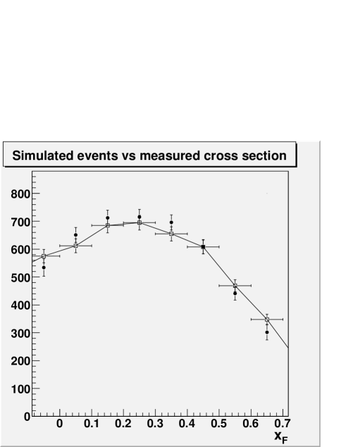
Figure 5: Filled squares: NA10 data at 194 GeV, for $\sqrt{\tau}$ in the range 0.33-0.36. Empty squares with joining line: Simulation (see text).

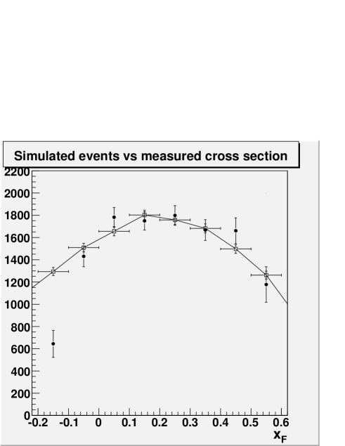
Figure 6: Filled squares: NA10 data at 286 GeV, for $\sqrt{\tau}$ in the range 0.33-0.36. Empty squares with joining line: Simulation (see text).

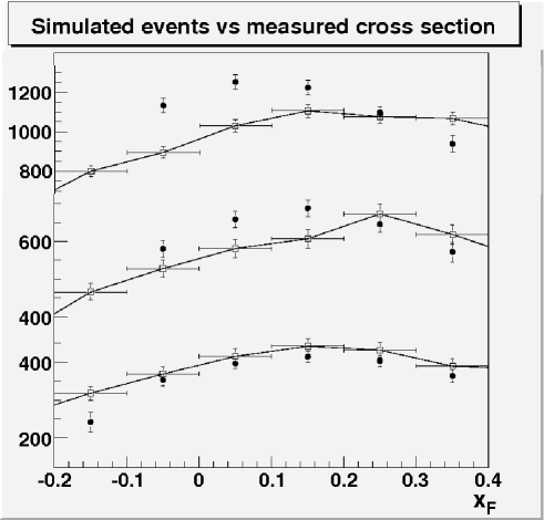
Figure 7: Filled squares: NA10 data at 286 GeV, for $\sqrt{\tau}$ in the ranges 0.21-0.24 (top), 0.24-0.27 (middle), 0.27-0.3 (bottom). Empty squares with joining line: Simulation (see text).

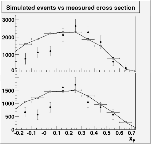
Figure 8: Filled squares: NA10 data at 286 GeV, for $\sqrt{\tau}$ in the ranges 0.51-0.54 (top) and 0.54-0.63 (bottom). These are equivalent to dilepton masses over the bottonium region. Empty squares with joining line: Simulation (see text).

Data in fig.5 come from NA10 (194 GeV beam), and the simulated events are a subset of 100,000 events sorted by DY_AB5 in the mass range 4-9 GeV/c², assuming a negative pion beam of 194 GeV hitting Tungsten. The data in figs. 6, 7 and 8 all refer to the upper energy beam of NA10, and their simulated counterparts have been extracted from a set of 100,000 events sorted between 4 and 7 GeV/c², of 100,000 events between 7 and 9 GeV/c², and of 50,000 events between 11 and 15 GeV/c².

For the lower energy beam (pions of 194 GeV, meaning $s$ $\approx$ 364 GeV²) fig.5 reports the $x_{F}$ distribution for $\sqrt{\tau}$ in the range 0.33-0.36, equivalent to dilepton mass between about 6.3 and 6.9 GeV/c².

Fig.6 considers the same $\sqrt{\tau}$ range, for the case of the upper energy beam (286 GeV, meaning $s$ $\approx$ 537 GeV²). In this case this corresponds to dilepton mass between 7.6 and 8.3 GeV/c². According with the scaling hyppothesis, the two data distributions should be the very similar in the $x_{F}$ range 0-0.6 covered by both measurements.

For $\sqrt{\tau}$ $<$ 0.3, the $x_{F}$ range covered by NA10 becomes small and data distributions are rather flat. Fig.7 reports data and simulations for the three $\sqrt{\tau}$ ranges 0.21-0.24, 0.24-0.27, 0.27-0.3, corresponding to masses ranging from 4.9 to 6.9 GeV/c².

The compared examination of the three sets of fig.7 suggests that (i) the simulation is worse for smaller $\sqrt{\tau}$, (ii) the $K-$factor extracted from E615 is slightly less steep (in its dependence on $\tau$) than the one extracted from NA10.

The former fact depends on the increasing relevance of sea values for $x_{projectile}$ at small masses. The default distribution for $x_{\pi}$ in DY_AB5 comes from E615 where sea (anti)quarks of the pion play a minor role in the fit of the pion distributions. For this reason, data from both NA10 and E615 are reasonably fitted for $x_{F}$ $>$ $-0.1$ with the exception of small-$\sqrt{\tau}$ distributions.

A signal of the relevance of sea partons from the pion side is the shift of the $x_{F}-$distribution peak towards $x_{F}$ $=$ 0. Valence-dominated measurements show this peak at $x_{F}$ $=$ 0.1-0.3. When the sea of the pion becomes relevant, it is probably better to substitute the default sea pion distribution of DY_AB5 with more recent ones. Fig.7 suggests that this may be the case for $\sqrt{\tau}$ below 0.25.

An interesting feature of NA10 is the presence of a conspicuous set of data at masses over the bottonium mass. This is $not$ the situation for which DY_AB5 has been thought, however it is interesting to try and simulate these events. Fig.8 reports data and simulation for $\sqrt{\tau}$ in the ranges 0.51-0.54 (mass between 11.8 to 12.5 GeV/c²) and 0.54-0.63 (mass between 12.5 and 14.6 GeV/c²).

We see that DY_AB5 has difficulties in reproducing the shape of these event distributions for $x_{F}$ $<$ 0.2. Actually, the “gap” of these data distributions at $x_{F}$ $\approx$ 0 looks a little unnatural. More in general, in all the previous figures the agreement between montecarlo and data is worse for negative $x_{F}$, where data distributions fall rather steeply. This could be related with the fact that negative $x_{F}$ data are at the border of the regions of good acceptance for fixed target experiments.

3.3 Sivers asymmetry plots in different calculation schemes

As observed in Section 2.5, the event cross section may be written in the form $\sigma$ $=$ $\sigma_{0}(X_{1},X_{2},P_{t},\theta)$ $[1+A(X_{1},X_{2},P_{t},\theta,..)]$, where the former term expresses that part of the cross section that does not contain azimuthal and spin asymmetries, while the asymmetries themselves are contained in $A$, and where $A$ may be approximated in different ways. In particular, in DY_AB5 $A$ contains flavor weight factors, that are absent a more recent version DY_AB6. In DY_AB6 the full cross section $\sigma$ is a sum of independent terms each referring to a sea or valence parton. Each flavor contribution carries “its own” asymmetry. In DY_AB5 $\sigma_{0}$ is a sum of flavor contributions, and $A$ is an independent sum of flavor contributions (see[14]), weighted with good sense.

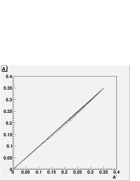
Figure 9: Scatter plot of asymmetries calculated by DY_AB5 (horizontal) and by DY_AB6 (vertical), for 7000 sorted $\pi^{-}p$ Drell-Yan events at $s$ $=$ 100 GeV², in the mass range 4-9 GeV/c². From [14].

Figure 10: Scatter plot of asymmetries calculated by DY_AB5 (horizontal) and by DY_AB6 (vertical), for 20000 sorted $\pi^{+}p$ Drell-Yan events at $s$ $=$ 100 GeV², in the mass range 1.5-2.5 GeV/c². From [14].

As far as azimuthal/spin asymmetries are neglected, the two codes produce the same results ($\sigma_{0}$ is the same in both cases). When asymmetries are included, the scheme implemented by DY_AB6 is more proper.

Exploiting the equality of $\sigma_{0}$ in the two cases, in [14] Drell-Yan events have been sorted according with $\sigma_{0}$ only, and the corresponding Sivers asymmetry (deriving from the $A$ term) has been calculated within the relations of DY_AB5 and of DY_AB6. The the scatter plot of the two asymmetry calculations for each event are reported in several figures. From that work two figures are borrowed, showing the two most “extreme” cases.

Fig.9 reports 7000 events for $\pi^{-}p$ Drell-Yan at $s$ $=$ 100 GeV², lepton invariant mass in the range 4-6 GeV/c², transverse momentum in the range 1-3 GeV/c. The Sivers asymmetry is parameterized according to [9].

Fig.10 reports 20000 events for $\pi^{+}p$ Drell-Yan at $s$ $=$ 100 GeV², lepton invariant mass in the range 1.5-2.5 GeV/c², transverse momentum in the range 1-3 GeV/c. The Sivers asymmetry is parameterized according to [25].

In the former case DY_AB5 and DY_AB6 would produce the same Sivers asymmetry. In the latter the difference is striking. As deeply discussed in [14] the difference between the two is proportional to the role of sea (anti)quarks. Positive pions on protons, and small dilepton mass, enhance the role of sea partons.

For these reasons, the code DY_AB6 has been prepared, aiming at situations where sea partons could become more and more relevant.

However, the use of DY_AB6 has been up to now restrained by the fact that the available parameterizations of functions like the Sivers one are normally produced by fitting data within the same “ideological” scheme of DY_AB5. In these cases, the use of DY_AB6 would increase errors, instead of decreasing them. This is discussed in [14] with plenty of details.

The main point is that when a “global fit” is undertaken using a scheme like the one of DY_AB5, the effect of sea partons is effectively included inside valence quark distributions. So, when the results from such a global fit are emploied in DY_AB6 for predicting some result, it is very dangerous to add separate sea quark contributions that are already present in valence quark distributions.

The place where DY_AB6 can be more proper is the one of $theoretical$ models for the Sivers function, built according with the scheme where each flavor is individually considered. But for the aim of modelling an experiment apparatus, one normally prefers using phenomenological parametrizations, rather than theoretical models.

References

- [1] S.D.Drell and T.M.Yan, Phys. Rev. Lett. 25 (1970) 316.
- [2] PANDA collaboration, L.o.I. for the Proton-Antiproton Darmstadt Experiment (2004), http://www.gsi.de/documents/DOC-2004-Jan-115-1.pdf.
- [3] GSI-ASSIA Technical Proposal, Spokeperson: R.Bertini, http://www.gsi.de/documents/DOC-2004-Jan-152-1.ps .
- [4] P. Lenisa and F. Rathmann [for the PAX collaboration], hep-ex/0505054.
- [5] R.Bertini, O.Yu Denisov et al, proposal in preparation.
- [6] see e.g. G.Bunce, N.Saito, J.Soffer, and W.Vogelsang, Ann.Rev.Nucl.Part.Sci. 50 525 (2000) [arXiv:hep-ph/0007218].
- [7] A.Bianconi and M.Radici, Phys.Rev. D 71 (2005) 074014.
- [8] A.Bianconi and M.Radici, Phys.Rev. D 72 (2005) 074013.
- [9] A.Bianconi and M.Radici, Phys.Rev. D 73 (2006) 034018.
- [10] A.Bianconi and M.Radici, Phys.Rev. D 73 (2006) 114002/1-11.
- [11] A.Bianconi, Phys.Rev.D (2006).
- [12] A.Bianconi, “Monte Carlo event generator DY_AB4 for Drell-Yan events with dimuon production in antiproton and negative pion collisions with molecular targets”, Internal note MUO-001 of the PANDA collaboration (2006), at http://www-panda.gsi.de/auto/doc/_home.htm.
- [13] M.Maggiora (for the ASSIA collaboration), “Spin physics with antiprotons”, preceedings of “Spin and Symmetry” conference, Prague 2005, Czech.J.Phys. 55, A75 (2005).
- [14] A.Bianconi and M.Radici, J. Phys. G: Nucl. Part. Phys. 34 No 7 (July 2007) 1595 (ArXiv:hep-ph/0610317).
- [15] D.Boer, PRD 60 (1999) 014012.
- [16] R.D.Field, “Applications of Perturbative QCD”, Addison-Wesley Publishing Company, 1989.
- [17] Conway et al, Phys.Rev.D 39 (1989) 92.
- [18] Anassontzis et al, Phys.Rev.D 38 (1988) 1377.
- [19] H.Shimizu, G.Sterman, W.Vogelsang, and H.Yokoya, Phys.Rev. D 71 (2005) 114007.
- [20] V.Barone, A.Drago, P.G.Ratcliffe, Phys.Report 359 (2002) 1.
- [21] E.L.Berger and S.J.Brodsky, Phys.Rev.Lett.42 940 (1979).
- [22] HEPDATA: the Durham HEP Database, cared by the Durham Database Group of the Durham University (UK). http://durpdg.dur.ac.uk/
- [23] J.C.Webb, Ph.D.Thesis, arXiv:hep-ex/0301031.
- [24] Ting-Hua Chang, Ph.D.Thesis, arXiv:hep-ex/0012034.
- [25] M.Anselmino et al, Phys.Rev.D72, 094007 (2005).
- [26] W.Vogelsang and F.Yuan, Phys.Rev.D72, 054028 (2005).
- [27] J.C. Collins, A.V. Efremov, K. Goeke, M. Grosse Perdekamp, S. Menzel, B. Meredith, A. Metz, and P.Schweitzer, Phys.Rev. D73 094023 (2006).
- [28] J.C.Collins and D.E.Soper, Phys. Rev. D 16 (1977) 2219.
- [29] D.Sivers, Phys.Rev. D41, 83 (1990); D.Sivers, Phys.Rev. D43, 261 (1991).
- [30] D.Boer and P.J.Mulders, Phys.Rev. D57, 5780 (1998).
- [31] B.Betev et, Zeit.Phys.C 28 9 (1985).
- [32] B.Betev, private communication to HEPDATA (previous ref.22).