Extraction of finite-energy contributions to the Sivers asymmetry from the analysis of exclusive proton-proton scattering.

Abstract

I study the effect of scalar and spin-orbit rescattering terms, in the production of a nonzero Sivers-like asymmetry in proton-proton collisions (inclusive production and Drell-Yan) at moderate center of mass energies $\sqrt{s}$ $<$ 15 GeV and transverse momentum up to 3 GeV/c. An ultrarelativistic generalization of the Glauber formalism is here used to (i) fit the scalar and spin-orbit interaction terms on proton-proton elastic scattering data, including analyzing power, (ii) transfer such information to inclusive proton-proton scattering. It is shown that the phenomenological interactions responsible for the nonzero analyzing power in proton-proton elastic scattering produce a relevant nonzero analyzing power in inclusive processes associated with proton-proton collisions. This could represent a relevant (possibly higher-twist) contribution to the Sivers asymmetry.

1 Introduction

1.1 General background

The problem of the study and measurement of T-odd distributions in hadron-hadron scattering has recently acquired a certain relevance and quite a few related experiments have been thought or scheduled for the next ten years[1, 2, 3, 4, 5].

In particular several studies and models have been proposed for the Sivers distribution function[6]. Its possible existence as a leading-twist distribution was demonstrated[7, 8, 9, 10] recently, and related[11] to previously studied T-odd mechanisms[12, 13]. Some phenomenological forms for its dependence on $x$ and $k_{T}$ have been extracted[14, 15, 16, 17, 18] from available data[19, 20, 21, 22, 23].

While studies of general properties[24, 25, 26, 27, 28, 29, 30, 31, 32, 33, 34, 35] of T-odd functions relate these functions with a wide spectrum of phenomena, quantitative models mostly follow the general scheme suggested in [7]. A known quark-diquark spectator model[36] is extended by including single boson exchange[37, 38, 39, 40]. In the case of [41] the unperturbed starting model was a Bag model, and for [42] a constituent quark model.

Here, I want to follow a different approach, that may be of interest in the case of intermediate energy measurements, and that relates Single Spin Asymmetries (SSA) in inclusive processes with SSA in exclusive processes.

A well measured SSA in an exclusive channel is the normal vector analyzing power measured in elastic proton-proton scattering at energy 20-30 GeV and $Q_{T}$ $=$ 1$-$3 GeV/c (see [43, 44, 45, 46, 47, 48]).

In the energy range 20-28 GeV, and for $Q_{T}-$ near 3 GeV/c, this observable is unexpectedly large and roughly energy-independent (see fig.8 later in this work). At energies over 30 GeV or $Q_{T}$ over 3 GeV/c it is not measured.

A nonzero analyzing power in $pp$ $\rightarrow$ $pp$ requires interference between helicity-flip and helicity non-flip amplitudes with 90^o phase difference (see e.g. [49] or [43] for reviews on this and related points). For this reason, in PQCD helicity-conserving processes this analyzing power must be very small, and the origin of the phenomenon has not yet a commonly accepted explanation. Attempts to explain it may be traced back to ref.[51] in a non-QCD context. For the region of semihard $Q_{T}$ $=$ 1$-$3 GeV/c many nontrivial models have been proposed[52, 53, 54, 55, 58, 57, 50, 56, 59, 60, 61, 62, 63, 64, 65, 66, 67], but a “standard” model, in the sense of a commonly accepted model for this effect, does not exist at present. It must be observed that for some of the previous models (e.g.[61]) the effect should persist at much larger energies than 30 GeV, while other ones select a preferential energy range, over which the effect should be suppressed.

The idea underlying the present work is that the interactions producing such an asymmetry are also active in inclusive processes originated by hadron-hadron collisions, at the same energy come and transferred momenta. In such a case, they could contribute to a nonzero asymmetry of Sivers-like kind. So a scheme can be imagined, allowing for information transfer from elastic proton-proton scattering to proton-proton inclusive processes. This is attempted in the following.

I do not propose nor adopt any model for the proton-proton elastic scattering amplitude. But I postulate a general form for a set of amplitudes contributing to this process at quark level. These amplitudes become initial state interactions in inclusive processes, where their presence admits for a nonzero Sivers asymmetry.

1.2 This work

The class of processes I want to consider here is the one of SSA in inclusive collisions between an unpolarized proton and a transversely polarized proton. In particular, azimuthal asymmetries in inclusive production of mesons or (virtual/real) photons. For fixed target experiments, the kinematics of interest is the one with moderate beam energy 10-60 GeV, and transverse momentum in the semihard regime 1-3 GeV/c.

To find nonzero T-odd quantities like the Sivers function one needs rescattering interactions between the active quarks and the surrounding particles. In particular, imagining that a hadron-hadron inclusive hard process is triggered by a hard collision between a quark in the projectile hadron (active quark) and a parton in the target hadron, this work is centered on the rescattering interactions between the active quark and the target hadron (initial state interactions, ISI).

First, I introduce a very simple bound state in light-cone coordinate representation for the active quark in the projectile proton. For this state, I speak of “unperturbed” bound state, where “unperturbed” means that it is not affected by ISI with the target hadron. This state will be a starting point for reproducing both inclusive and exclusive processes. It is a two-component state (each component representing positive or negative transverse quark spin). In Appendix A it is shown that in ultrarelativistic conditions these two components contain all the relevant independent information on the quark state.

Before the hard scattering event, this state is affected by ISI. The precise form and the parameter values for ISI are extracted from the phenomenology of elastic proton-proton scattering in semihard conditions. I assume that the interactions producing a nonzero analyzing power in proton-proton elastic scattering at the required kinematics may be rewritten in terms of interactions between a projectile quark and a target hadron, where the former is bound to a projectile hadron, and the latter has a continuous structure.

The scheme used for this aim is an ultrarelativistic generalization of the Glauber method[69]. Starting from the fact that the fitted data include unpolarized scattering and single normal spin analyzing power, consideration of the number of constrained amplitudes reduces the considered ISI to a sum of scalar and spin-orbit interaction terms, in a 2x2 formalism.

Fitting parameters on proton-proton data does not allow for a strict flavor separation. However, it implies u-quark dominance. So in the following the expression “quark interactions” mainly means “u-quark interactions”.

In Section II, some general definitions are presented and discussed, in particular the definitions of unpolarized quark distribution and Sivers-like analyzing power, in terms of empiric variables on the one side and of quark operators on the other side. Also, the quark unperturbed bound state in coordinate representation is introduced. Some related details are put into Appendix A section.

In Section III, an operator describing ISI is introduced. Having to modify the above two-component state, this operator consists of a 2x2 matrix operator, that is written in eikonal form as the exponential of a set of scalar plus spin-orbit matrices.

I describe and discuss the theoretical foundations and several details of the method allowing me to extract the form and parameters of the ISI operator from elastic proton-proton scattering and to apply it to the calculation of inclusive quark distributions. Some details are put into Appendix B Section.

In Section IV the parameters of the ISI operator are fitted to reproduce data on proton-proton elastic scattering at beam energy 20$-$50 GeV and transferred momentum 1$-$3 GeV/c, and MRST[70] unpolarized u-quark collinear distribution at $Q^{2}$ $=$ 16 GeV².

In Section V the rescattering operator is used to calculate the unpolarized quark distribution, including Sivers-like asymmetry, for $x$ in the valence region and transverse momenta up to 3 GeV/c.

It must be remarked that this work is subject to some limits:

1) Computational limits. I face stability problems in calculating Fourier transforms for transverse momenta over 3 GeV/c (elastic scattering) or 2.7 GeV/c (inclusive at $x$ $=$ 0.3). These problems get worse at increasing x, so my analysis centers at $x$ $=$ 0.3. This value guarantees that we are in the valence region, and that numerical results are reliable.

2) Limitedness of the data set used for fixing the parameter values. Proton-proton scattering is not the only exclusive process from which information on rescattering in hadron-hadron hard processes may be extracted, although it represents the most complete and precise set of available data in this respect.

3) Twist identification. The formal apparatus introduced here implies leading twist results at the condition that the key parameters of the interaction operator become energy-independent at large energies. Since there is presently no way to decide how these parameters behave asymptotically, it is not possible to establish whether the found effect is a leading or a higher twist one. If it is a relevant higher twist, it should become negligible (compared to leading twist effects) at energies like 100 GeV. Exploiting the fact that the measured analyzing power is energy-independent from 20 to 30 GeV, I assume that the considered interactions are relevant in the energy range 10-60 GeV. For what happens over this range, I cannot formulate hypotheses.

Here the terms “Sivers asymmetry” and “Sivers effect” are preferred to “Sivers function”. The last one is appropriate in the case of a leading twist contribution. To conform with common notation, in the result section I will name “Sivers function” a quantity that may be extracted from single spin asymmetries in inclusive processes. This quantity must be meant as a measured function, whose theoretical interpretation may be and may be not the one of a Sivers function.

As a last remark, data and distributions shown in figs. 6, 7, and 8, together with the original references, have been reconstructed thanks to the Durham HEP database[71].

2 The general scheme - no rescattering.

2.1 Basic variables.

Apart for some points where it is clearly specified, all variables will refer to the center of mass of the colliding hadrons. Let $\vec{b}$ $=$ $(b_{x},b_{y})$ be the quark impact parameter and $\vec{k}_{T}$ $=$ $(k_{x},k_{y})$ the transverse momentum conjugated with it. Let $P_{+}$ be the large light-cone component of the hadron momentum, so that $xP_{+}$ is the quark $(+)$ momentum conjugated with $z_{-}$. Assuming by default the validity of a standard factorization scheme[72, 73], the fourth coordinate $z_{+}$ plays no role and is fixed to zero.

I substitute $z_{-}$ with the rescaled coordinate

$$\xi\ \equiv\ P_{+}z,\hskip 14.22636pt\rightarrow\hskip 14.22636ptP_{+}\int dz_{-}exp(-ixP_{+}z_{-})\ =\ \int d\xi exp(-ix\xi)$$ (1)

not to work with a singularity of the Fourier transform in the infinite momentum limit $P_{+}$ $\rightarrow$ $\infty$.

Contrary to the ordinary treatment of the problem, where one works on a two-point correlation operator deriving from a set of squared one-point amplitudes, I develop most of the work at the level of one-point amplitudes, square them and then sum over the relevant states.

Since the inclusive process is described here in terms of squared amplitudes, and these amplitudes are calculated before being squared, $\xi$ is not bound to be positive, as it happens in the ordinary treatment based on a two-point correlator with intermediate real states. In that case $\xi$ has the meaning of the difference between the light-cone positions of two points. In this work it describes the light-cone position of one of the two only.

2.2 Two-component transverse spin formalism.

I consider a quark inside a hadron with a given spin projection $S_{y}$ $=$ $+1/2$. The quark is supposed to present a nonzero transverse momentum along the $\hat{x}$ direction, and is described by a two-component quark spinor

$$\vec{\psi}\ \equiv\ (\psi_{+},\psi_{-}).$$ (2)

These two components are the components of the full 4-spinor $\Psi$ describing a free quark on two 4-spinors $\Psi_{T+}$, $\Psi_{T-}$:

$$\Psi\ \equiv\ \psi_{+}\Psi_{T+}\ +\ \psi_{-}\Psi_{T-}$$ (3)

where

$$\Psi_{T+}\ \approx\ (\vec{\phi}_{+},\vec{\phi}_{-}),\ \Psi_{T-}\ \approx\ (\vec{\phi}_{-},\vec{\phi}_{+})$$ (4)

and $\vec{\phi}_{\pm}$ are 2-component eigenstates of

$$\hat{\sigma}_{y}\vec{\phi}_{\pm}\ =\ \pm\phi_{\pm}.$$ (5)

where the scattering plane is formed by the directions “z” (longitudinal) and “x” (transverse).

In the Appendix A section it is demonstrated (i) that in the ultrarelativistic limit the above transverse spinors give a full description of the state of a free quark, (ii) that

$$\bar{\Psi}\gamma_{+}\Psi\ \approx\ |\psi_{+}|^{2}\ +\ |\psi_{-}|^{2},$$ (6)

that becomes an equality in the u.r. limit. The $\gamma_{+}-$projection produces the distribution functions associated to an unpolarized quark with positive $z-$direction in an infinite momentum frame.

2.3 TMD quark distribution and Sivers-like analyzing power

I consider the transverse momentum dependent (TMD) quark distribution $q(x,\vec{k}_{T})$ of unpolarized quarks in a hadron with $y-$polarization $+1/2$. This may be defined in a phenomenological and in a theoretical way.

The phenomenological definition adopted here is in agreement with the so-called “Trento convention” [74], in which the unpolarized quark transverse momentum dependence distribution has the form

$$q(x,\vec{k}_{T})\ \equiv\ q_{U}(x,k_{T})\ -\ 2{{\vec{S}\wedge\vec{k}_{T}\cdot\hat{z}}\over M}q_{S}(x,k_{T})=\ q_{U}(x,k_{T})\ \pm\ {k_{x}\over M}q_{S}(x,k_{T})$$ (7)

for an unpolarized quark in a hadron with $\vec{S}$ $=$ $\pm\hat{y}$, moving along the $z$ direction.

If the second term is scale-independent, $q_{S}$ is the Sivers function. In the following I will speak of “Sivers asymmetry” meaning $q_{S}k_{x}/2Mq_{U}$.

This asymmetry can of course be isolated by calculating the ratio $[q_{+}(k_{x})-q_{-}(k_{x})]/[q_{+}(k_{x})+q_{-}(k_{x})]$ corresponding to opposite proton polarizations. Alternatively, one may use the difference $q_{+}(+k_{x})$ $-$ $q_{+}(-k_{x})$ for fixed proton polarization. The result is the same.

So, the center of this work will be the quark distribution asymmetry $A(x,k_{x})$, defined as

$$A(x,k_{x})\ \equiv\ \Bigg{(}{{q(x,k_{x})-q(x,-k_{x})}\over{q(x,k_{x})+q(x,-k_{x})}}\Bigg{)}_{k_{y}=0}$$ (8)

In the following, this inclusive analyzing power of the quark distribution will be simply indicated as “Sivers asymmetry”, or simply “asymmetry”.

2.4 Sivers-like asymmetry in terms of two-component quark states

On the theoretical side, $q(x,\vec{k}_{T})$ may be defined as the $\gamma_{+}-$projection of the two-point correlation function $C(x,\vec{k}_{T})$

$$q(x,\vec{k}_{T})\ =\ Tr[\gamma_{+}C(x,\vec{k}_{T})],$$ (9)

$$C(x,\vec{k}_{T})\ =\ \int d\xi d^{2}b\ e^{-ix\xi+i\vec{k}_{T}\cdot\vec{b}}<P|\Psi(0)\bar{\Psi}(0_{+},\xi,\vec{b})|P>$$

$$\propto\ \sum_{n}|\psi_{n}(x,\vec{k}_{T})|^{2}.$$ (10)

In this work, the strategy will not be a direct calculation of $C(x,\vec{k}_{T})$ from the definition eq.2.4, but a calculation of a restricted number of amplitudes $\psi_{n}(x,k_{T})$ in eq.10. These are later squared and summed to obtain the correlator. This choice is associated with the need of introducing ISI that have continuous and nonperturbative character.

The functions $\psi_{n}$ $=$ $<n|\hat{q}(x,\vec{k}_{T})|hadron>$ must be read as quark distribution amplitudes, i.e. amplitudes for removing a quark with quantum numbers $x,\vec{k}_{T}$ from the initial hadron leaving the spectator in the state $|n>$. In any single-particle model for a set of bound quark wavefunctions, the above $\psi_{n}(x,\xi)$ coincides with one of the single quark bound state wavefunctions in the infinite momentum frame. The joint action of the $\gamma_{+}-$projection, and of the light-cone limit condition $z_{+}$ $=$ 0 (equivalent to integration of the quark wavefunction over $k_{-}$) selects the correct subspace in the u.r. limit.

If the states $\psi_{n}$ of eq.10 are written in the form of eq.3, exploiting eq.6 I get

$$q(x,\vec{k}_{T})\ =\ Tr[\gamma_{+}C(x,\vec{k}_{T})]\ \propto$$

$$\propto\ \sum_{n}Tr(\bar{\psi_{n}}\psi_{n}\gamma_{+})=\ \sum_{n}\bigg{(}|\psi_{+}(x,\vec{k}_{T})|^{2}\ +\ |\psi_{-}(x,\vec{k}_{T})|^{2}\bigg{)}_{n}.$$ (11)

where $\psi_{\pm}(x,\vec{k}_{T})$ are complex functions (and not 4-spinors anymore) representing the projections of the quark wavefunction on transverse spin states. Inserting eq.11 in eq.8 the asymmetry may be written as

$$A(x,k_{x})\ \equiv\ {{\sum_{n}\bigg{(}|\psi_{+}(x,\vec{k}_{T})|^{2}\ -\ |\psi_{-}(x,\vec{k}_{T})|^{2}\bigg{)}_{n}}\over{\sum_{n}\bigg{(}|\psi_{+}(x,\vec{k}_{T})|^{2}\ +\ |\psi_{-}(x,\vec{k}_{T})|^{2}\bigg{)}_{n}}}.$$ (12)

2.5 The undistorted quark state

In this work one state $n$ only is considered, so that the spinor $\vec{\psi}$ $\equiv$ $(\psi_{+},\psi_{-})$ represents the splitting of the (polarized) hadron into a quark with spin projection $\pm\hat{y}$ and spectator in this unique state $|n>$.

To later insert initial state interactions, we need to express the quark state in space-time representation:

$$\vec{\psi}(x,\vec{k}_{T})\ \equiv\ \int d\xi d^{2}be^{-ix\xi}e^{i\vec{k}_{T}\cdot\vec{b}}\vec{\psi}(\xi,\vec{b}),\hskip 14.22636pt\vec{\psi}(\xi,\vec{b})\ \equiv\ \left(\begin{array}[]{cc}\psi_{+}(\xi,\vec{b})\\ \psi_{-}(\xi,\vec{b})\end{array}\right)$$ (15)

I assume that the state $\vec{\psi}(\xi,\vec{b})$ is defined by a given value of the the quark total angular momentum $\vec{J}$ in the hadron rest frame, and that in this state a nonzero correlation $<\vec{S}_{hadron}\cdot\vec{J}_{quark}>$ $=$ $+1/4$ is present. In other words, the quark $\vec{J}$ coincides with the parent hadron spin.

A nonzero correlation between the hadron spin and the quark total angular momentum is necessary, since a spin-related effect is impossible if a quark transports no information on the parent hadron spin. In absence of ISI this correlation would produce a nonzero transversity, but not a single-spin asymmetry of naive Time-odd origin because of global invariance rules.

In absence of ISI, we may assume that we are able to calculate the Fourier transform eq.(15) and write it directly in impact parameter representation as ($PW$ means “plane wave”, i.e. ISI-undistorted state)

$$\vec{\psi}(\xi,\vec{b})_{PW}\ \equiv\ \phi(\xi)\phi^{\prime}(\vec{b})\cdot|J_{y}\ =\ +1/2>$$ (16)

A state with given $J_{y}$ may be realized via S and P waves, corresponding to the scalar and axial vector spectators of [36].

In this work I have avoided, as much as possible, the introduction of parameters that cannot be constrained by data. Since elastic proton-proton data may be reasonably fitted using a pure S-wave state (see section IV), I have limited myself to the state:

$$\vec{\psi}(\xi,\vec{b})_{PW}\ \equiv\ \phi(\xi)\phi^{\prime}(b)\left(\begin{array}[]{cc}1\\ 0\end{array}\right)$$ (19)

where $\phi(\xi)$ and $\phi^{\prime}(b)$ have Gaussian shapes.

The width $\Delta\xi$ of $\phi(\xi)$ has been chosen comparing the $k_{T}$ $=$ 0 distribution with the shape of the collinear function $u(x)$ as given by MRST[70] at the scale $Q^{2}$ $=$ 16 GeV².

After an initial fit performed in absence of ISI, the fit has been re-tuned again after ISI had been included. The final fit is shown in fig.6, and has been performed with gaussian width parameter $\Delta\xi$ $=$ 4.5, plus all the later discussed parameters.

Although the full procedure is recursive, and so no parameter is fully independent from the other ones, I may say that the fit on the MRST collinear distribution is decisive to establish the width of $\phi(\xi)$, within small corrections. As discussed in section IV, longitudinal parameters cannot be extracted from elastic data (this is evident from eq.25). On the contrary, the width of $\phi^{\prime}(b)$ and all the rescattering parameters are constrained by elastic data (see section IV).

3 Insertion of initial state interactions (ISI)

3.1 Basic assumptions of this work

Assumption 1)

a set of independent quark-quark interactions is responsible for hadron-hadron scattering at $E$ $=$ 10-60 GeV, transferred momenta $Q_{T}$ $=$ 1-3 GeV/c.

Assumption 2)

the same interactions produce initial state distortions of the wavefunction of a projectile quark passing through or near a target hadron in hadron-hadron inclusive processes, at the same energy.

Here the word “quark” may also mean “antiquark”. Individual quark-quark interactions are imagined as exchanges of multigluon sets, that is not trivial to reproduce via resummed perturbative calculations. Assumption (1) receives support from e.g. the data of [77] for small$-Q_{T}$ scattering, and should be reasonable for $Q_{T}$ $\approx$ 2$-$3 GeV/c. Assumption (2) becomes reasonable if interpreted in non-exhaustive sense: interactions deduced from elastic proton-proton scattering data constitute one of the relevant contributions to ISI in inclusive processes.

3.2 Basic equations: Scattering between a quark and a composite hadron

To connect exclusive and inclusive processes, here an ultrarelativistic generalization of the Glauber formalism is used.

In Appendix B below, a comparison of the steps leading to the nonrelativistic and ultrarelativistic forms of the Glauber-distorted quark wavefunction is presented, together with a discussion of the most relevant high energy corrections[83].

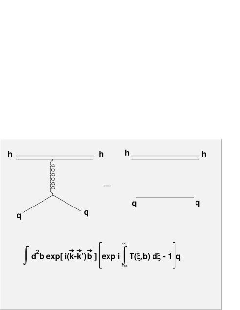
Figure 1: quark-hadron scattering amplitude in Glauber u.r. approximation. The gluon-shaped t-channel exchange reproduces $all$ the terms contributing to the scattering, including the no-scattering term that is subtracted on the right side. The amplitude for this graph in Glauber approximation (scalar form) is proportional to the one in the figure (see text and eq.20).

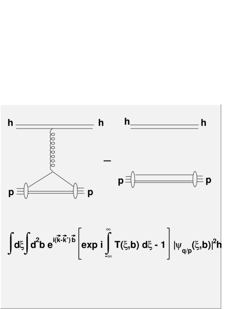
Figure 2: proton-hadron scattering amplitude in the same approximation as for the previous fig.1. The main difference, evident in the (scalar) expression for the amplitude reported in the figure, is the average over the quark bound state in the projectile hadron. For details, see text and eq.25.

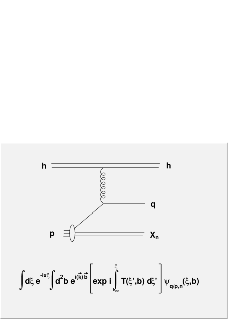
Figure 3: The ISI-modified quark distribution amplitude. The corresponding (scalar) amplitude is reported in the figure. For more precise details, see text and eq.26. Notice that in this case the “$-1^{\prime\prime}$ subtraction is not needed, since the no-rescattering term gives a leading contribution to the amplitude.

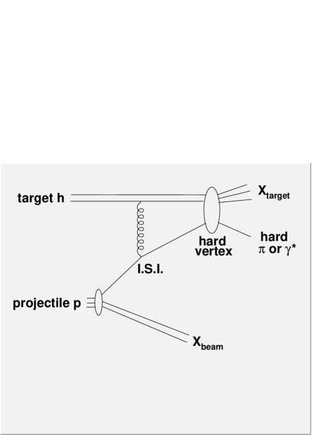
Figure 4: The full diagram for inclusive production. The blob near the right-upper corner is the true hard interaction characterizing the process, also in absence of rescattering. The gluon-shaped exchange represents all ISI terms, including the no-rescattering one.

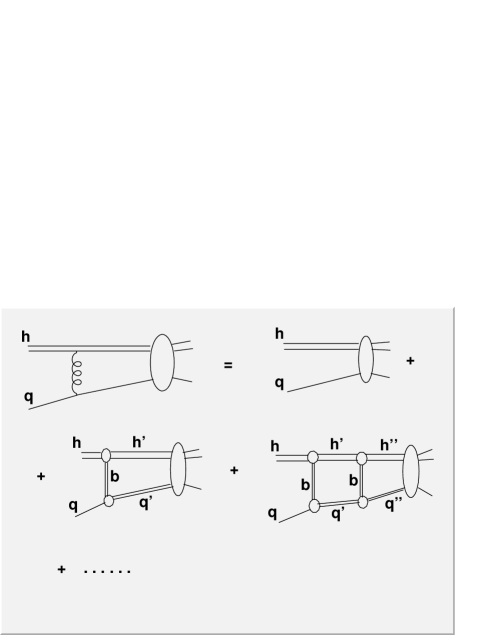
Figure 5: The structure of the ISI, attached to the hard scattering blob. T-channel double-line exchanges represent non-reducible sets of gluon, multigluon, meson, pomeron, etc exchanges. S-channel double lines represent intermediate states where the projectile quark (or the target hadron) is converted into a more complex intermediate state, like $q+g$ or $q+\bar{q}q$. In absence of these intermediate excited states the rescattering operator would be hermitean. The excited states in the last step (i.e. attached to the hard scattering blob) cause a “direct” imaginary part of the mean field, the other ones cause an “optical” imaginary part (see text, section III.3 and Appendix B).

The connection between the amplitudes for describing quark-hadron interaction, hadron-hadron interactions, and rescattering distortions of the quark distribution amplitude, is illustrated in figs.1, 2 and 3. The discussion of this section refers to these figures. The (slightly) simplified formulas shown the figures refer to the scalar interaction case, while a 2x2 matrix interaction operator is considered in the following text and equations.

As a consequence of assumption (1), the elastic scattering amplitude between a free quark and a bound quark in a hadron (fig.1) can be written as

$$T_{el,quark}(k_{o},q)\ =\ f(k_{o})\int d^{2}be^{i\vec{q}\cdot\vec{b}}\vec{\chi}_{f}^{+}\Bigg{\{}exp\bigg{[}i\hat{P}\int_{-\infty}^{\infty}\hat{T}(\vec{b},\xi)\bigg{]}\ -\ 1\Bigg{\}}\vec{\chi}_{o},$$ (20)

$$\hat{T}(\vec{b},\xi)\ \equiv\ \rho(\vec{b},\xi)\hat{T}^{\prime}(k_{o}).$$ (21)

These relations describe an average of the quark-quark scattering amplitude over the target structure. In eqs. 20 and 21:

-) The coefficient $f(k_{o})$ is a convention-dependent kinematic factor.

-) $\vec{k}_{o}\hat{z}\mp\vec{q}$ is the initial/final momentum of the free quark, $\vec{q}$ is the transferred momentum, $\xi$ is a longitudinal or a light-cone coordinate, $\hat{P}$ indicates path-ordered integration along a constant$-\vec{b}$ light-cone path.

-) The 2-spinors $\vec{\chi}_{o}$, $\vec{\chi}_{f}$ assign the initial/final spin of the projectile quark. These asymptotic spinors are defined $not$ to contain the spacetime dependence of the quark wavefunctions. In other words, the initial/final wavefunctions for the (free) projectile quark have the form $\vec{\chi}_{i,f}e^{i(k_{o}\xi\pm{{\vec{q}}\over 2}\cdot\vec{b})}$. (these will have to be generalized later, when we bound the projectile quark to a projectile hadron).

-) $\hat{T}(\vec{b},\xi)$ is a 2x2 matrix in the normal spin space. $\hat{T}^{\prime}(k_{o})$ is the 2x2 matrix of $forward$ scattering amplitudes between a projectile quark with momentum $k_{o}$ and a target quark at rest. $\hat{T}^{\prime}$ depends on $k_{o}$ only. The composition of the target proton in terms of individual quarks is contained in the single-particle density function $\rho(\vec{b},\xi)$.

The target density function $\rho(\vec{b},\xi)$ derives from an averaging procedure[69] over all the spectator degrees of freedom of the target:

$$exp\bigg{[}i\int_{-\infty}^{\infty}d1\ \hat{T}(1)\bigg{]}\ \sim\$$

$$\sim\ \int d2d3....|\psi_{target}(2,3,...)|^{2}exp\bigg{[}i\int_{-\infty}^{\infty}d1\ \hat{U}(1-2,1-3,...)\bigg{]}\$$ (22)

Since here the structure of the target only enters through the averaged operator $\hat{T}(1)$, in the following I work directly with this operator. For this reason it is proper to speak of a “mean field” treatment.

Eq.20 is pictorially represented by fig.1, where the “gluon-shaped” boson exchange must not be meant as a single gluon exchange: it represents the $full$ set of possible interactions between a single quark and a hadron, approximated by the exponential factor in eq.20.

In particular, the exponential factor (represented by the first diagram in fig.1) also includes the no-interaction term, as evident from the fact that it becomes unity for $\hat{T}$ $=$ 0. For this reason, it is necessary to subtract the diagonal contribution “$-1$”.

3.3 Basic equations: distortion of the wavefunction of a free projectile quark.

The key point is the possibility to rewrite the first term of the right-hand side of eq.20 (i.e. the term that does not contain the “$-1$” subtraction) in the form

$$f(k_{o})<\psi_{f}^{out}(\xi,\vec{b})|\psi_{o}^{in}(\xi,\vec{b})>\equiv\$$

$$\equiv f(k_{o})\int d\xi\int d^{2}b\ \cdot\ e^{-i(k_{o}\xi-{{\vec{q}}\over 2}\cdot\vec{b})}\vec{\chi}_{f}^{+}exp\bigg{[}i\hat{P}\int_{\xi}^{\infty}\hat{T}(\vec{b},\xi)d\xi\bigg{]}$$

$$e^{i(k_{o}\xi-{{\vec{q}}\over 2}\cdot\vec{b})}exp\bigg{[}i\hat{P}\int_{-\infty}^{\xi}\hat{T}(\vec{b},\xi)d\xi\bigg{]}\vec{\chi}_{o}$$ (23)

so that we may define the concept of “distorted quark wavefunction”, with the $\xi-$dependent distortion factor

$$F(\vec{b},\xi)\ =\ exp\bigg{[}iP\int_{-\infty}^{\xi}\hat{T}(\vec{b},\xi)d\xi\bigg{]}.$$ (24)

The connection between eqs.20 and 24 is a standard step in the Glauber approximation. Within a nonrelativistic formalism it was first used in [69], where also the spin-orbit case was discussed.

3.4 Basic equations: hadron-hadron scattering

Now two relevant generalizations are possible. First, we may substitute the wavefunction of a free projectile quark with the wavefunction of a quark that is bound to a projectile proton with momentum $p\hat{z}\pm\vec{q}/2$ (fig.2). In this case the scattering amplitude is (apart for an overall kinematic factor)

$$T_{EL}(p,q)=\ \int d\xi\int d^{2}b$$

$$\vec{\psi}^{+}(\xi,\vec{b})e^{i\vec{q}\cdot\vec{b}}\Bigg{\{}exp\bigg{[}i\hat{P}\int_{-\infty}^{\infty}\hat{T}(\xi,\vec{b})d\xi\bigg{]}\ -\ 1\Bigg{\}}\vec{\psi}(\xi,\vec{b})$$ (25)

and it describes the scattering between a projectile proton and a target hadron, for $q$ $<<$ $p$. In the following, this amplitude is used to fit a reasonable form for the $\hat{T}$ operator starting from data on angular distribution and normal analyzing power in elastic proton-proton scattering at beam energies 20-50 GeV.

The role of the “$-1$” subtraction must be stressed. It means that the leading scattering term is part of the interaction eikonal operator of eq.25. In the limit of no interaction the above amplitude is zero. If the “$-1$” factor is removed, in the limit of no interaction the above equation gives the nonperturbative expression of the projectile form factor $<\psi(p+q/2)|\psi(p-q/2)>$. In this case the eikonal operator may only contain second order corrections to the form factor, and the “hard” features of the scattering event, if present, must be inserted into the large-momentum tail of the bound state wavefunction. In this work we adopt the “$-1$” subtraction, suitable to describe semihard elastic scattering with $q$ $<<$ $p$. This means to assume that the bound state itself does not contain hard momentum tails.

3.5 Basic equations: DWBA and the modifications of the quark distribution functions.

The other useful generalization is the application of the distortion factor to the calculation of the quark distribution function, illustrated in fig.3. It exploits the Glauber approximation within the Distorted Wave Born Approximation (DWBA) scheme. In DWBA a matrix element of the form $<f|(A+B)|i>$, with $A$ and $B$ interaction operators, is written as $<f^{\prime}|B|i^{\prime}>$, where $|i^{\prime}>$ and $|f^{\prime}>$ are solutions of the problem where the interaction $B$ is excluded while $A$ is considered. This allows for a compared study of different processes whenever one may assume that the underlying distorting factors $A$ have the same origin. The procedure is of course justified if $B$ is harder than $A$.

The ISI-distorted quark distribution amplitude is

$$\vec{\psi}_{n}(x,\vec{k}_{T})=\ \int d\xi\int d^{2}be^{-ix\xi+i\vec{k}_{T}\vec{b}}exp\bigg{[}i\hat{P}\int_{-\infty}^{\xi}\hat{T}(\xi,\vec{b})d\xi\bigg{]}\vec{\psi}_{n,PW}(\xi,\vec{b})$$ (26)

where $\vec{\psi}_{n,PW}(\xi,\vec{b})$ is the amplitude for extracting a light-cone quark in position $(z_{-},z_{+},\vec{z}_{T})$ $=$ $(P_{+}\xi,0,\vec{b})$ while leaving the spectator in the state $|n>$, in absence of ISI. In this work $\vec{\psi}_{n,PW}(\xi,\vec{b})$ coincides with the quark bound state given by eq.19. For a generic nonzero $\hat{T}(\xi,\vec{b})$, eq.26 defines the quark distribution amplitude that enters eqs. 11 and 12 in presence of ISI.

It must be noted that the “$-1$” factor is missing in eq.26, since the undistorted term is a leading contribution in this case. In other words, for $\hat{T}(\xi,\vec{b})$ $=$ 0 the right hand side of eq.26 is anyway nonzero and coincides with the ISI-not-affected quark distribution amplitude $\vec{\psi}_{n,DW}(\xi,\vec{b})$.

As in figures 1 and 2, the gluon-shaped factor of fig.3 represents the eikonalized full set of rescattering interactions. Since we are speaking of “rescattering”, these do $not$ include the true hard scattering event defining the process class (Drell-Yan, meson production, etc). To stress this point, in fig.4 I show the amplitude for the full process interesting here. The “strictly hard” event is contained in the upper-right blob from which a hard line representing a jet, a meson or a massive photon emerges. The gluon-shaped ISI include everything softer than the final hard event.

3.6 Complex mean field

With the aim of arriving to a nonzero Sivers asymmetry, it is important that the rescattering operator contains different terms able to introduce phase shifts between competing amplitudes for the same process: $\hat{T}$ $=$ $\sum\hat{T}_{i}$. A special role in this respect is played by anti-hermitean interaction terms. I will simply speak of “real” and “imaginary” terms to mean hermitean and anti-hermitean 2x2 interaction matrices $\hat{T}_{i}$.

In fig.5 the gluon-shaped ISI of fig.4 are expanded in terms of non-reducible t-channel exchanges. Intermediate s-channel states that in fig.5 are named $q^{\prime}$, $q^{\prime\prime}$, etc, are in general more complex than quark states (e.g. a quark may split into quark+gluon, and the gluon may be absorbed in the next vertex). The presence of imaginary terms is related with the additional cuts that may be applied to these intermediate states.

The imaginary terms may have two origins[82, 69, 83]: direct and optical.

The direct one is the case where the underlying quark-quark scattering amplitude $\hat{T}^{\prime}$ is complex, and the process is single-scattering dominated. Since the described mean field is an average of $\hat{T}^{\prime}$ over the target matter distribution, a complex $\hat{T}^{\prime}$ leads to a complex mean field. This mechanism is surely present in the problem under consideration, and corresponds to the single rescattering graph in fig.5 when $q^{\prime}$ $\neq$ $q$ or $h^{\prime}$ $\neq$ $h$.

The optical case requires a two-step transition, and is the case where the initial state is regenerated after passing through an intermediate inelastic channel. Then, the existence of a cut in the intermediate state produces the imaginary part. This corresponds to taking the last contributing diagram in fig.5 with $q^{\prime\prime}$ $=$ $q$, $h^{\prime\prime}$ $=$ $h$, but $q^{\prime}$ or $h^{\prime}$ different from $q$ or $h$. The effective imaginary part is then present in $\rho(b,\xi)$. This optical effect may be defined of Gribov’s kind[83] (see Appendix B). The well-known optical effect of Feshbach’s kind[82] implies the formation of bound $q+h$ states but is suppressed in the short wavelength regime considered here.

A complex interaction term implies flux nonconservation. Obviously one expects absorption of flux from the initial state. To conserve unitarity, this lost flux will be redistributed among all the other accessible states. This implies opposite-phase imaginary terms dominating at small and large angles in the elastic channel. At small angles, we have some elastic scattering due to diffraction, but the net effect on the incoming flux is absorption, meaning a negative imaginary part for the interaction term. At large angles, second order transitions “elastic $\rightarrow$ inelastic $\rightarrow$ elastic” produce elastic flux. In a single channel approach, this is reproduced by a complex interaction term with positive imaginary part. The signature of this is the minimum in the data of fig.7 at $Q_{T}$ $=$ 1.2 GeV/c.

3.7 Selected interaction terms

The determination of $\hat{T}$ $\equiv$ $\rho(\xi,b)\hat{T}^{\prime}(k_{o})$ entering eqs. 20,21 is not unique, since different $\hat{T}(b,\xi)$ may lead to the same $\hat{T}_{\infty}(b)$ $\equiv$ $\int_{-\infty}^{\infty}\hat{T}(b,\xi)d\xi$. In addition, this operator derives from the averaging procedure eq.22 that is under control for simple few-body systems only (see [81] for a borderline example). So, in cases like the one interesting here one is obliged to guess and fit directly some model form for $\hat{T}(\xi,b)$.

I assume that the distorting factor $\hat{F}$ of eq.(24) does not present a fast dependence on $x$, so in fourier transforms in may be considered as $x-$independent. This assumption breaks down at small $x$, but that region is of no interest here since it clearly involves a different physics under several points of view. In numerical calculations, the path-ordered exponential operator is approximated by a quasi-continuous product:

$$exp\Bigg{(}i\hat{P}\int_{-\infty}^{\xi}\hat{T}(\xi^{\prime},\vec{b})d\xi^{\prime}\Bigg{)}\ \approx\ \prod(1+i\hat{T}d\xi)$$ (27)

where the product starts from a negative and large enough $\xi^{\prime}$ value where interactions may be neglected, and stops at $\xi$. The $\hat{T}$ matrix is a sum of the kind

$$\hat{T}\ =\ \sum\hat{T}_{scalar}\ +\ \sum\ \hat{T}_{spin-orbit}.$$ (28)

where two scalar ant two spin-orbit terms are included, and each term has the form:

$$\hat{T}_{scalar,n}\ \equiv\ \delta_{n}\left(\begin{array}[]{cc}1&0\\ 0&1\end{array}\right)\rho(\xi)\rho_{n}^{\prime}(b).$$ (31)

$$\hat{T}_{spin-orbit,n}\ \equiv\ \alpha_{n}\left(\begin{array}[]{cc}b_{x}&ib_{y}\\ -ib_{y}&-b_{x}\end{array}\right)\rho(\xi)\rho_{n}^{\prime}(b).$$ (34)

All the density functions have been chosen with gaussian form, normalized to $\rho_{i}(0)$ $=$ 1. The longitudinal density $\rho(\xi)$ is the same for all terms and is equal to the squared quark distribution amplitude $|\phi(\xi)|^{2}$ introduced in eq.19. In the following 3 transverse density gaussian functions $\rho_{n}^{\prime}(b)$ will be needed: a soft, a semi-hard and a ultra-hard one. In all, I will introduce a soft and a semi-hard scalar term, and a soft and a ultra-hard spin-orbit term. The $\delta_{n}$ coefficients are complex, while the $\alpha_{n}$ have been chosen as pure imaginary. See next section for details on the fitting procedure and for their values.

To see that the $O(\alpha_{n})$ terms are spin-orbit terms, I remark that the above matrices act on a basis of eigenstates of $\hat{S}_{y}$. This means that $\hat{S}_{y}$ $=$ $\sigma_{3}$, $\hat{S}_{z}$ $=$ $\sigma_{1}$, $\hat{S}_{x}$ $=$ $\sigma_{2}$ (apart for a factor 1/2). So we may rewrite:

$$\hat{T}_{spin-orbit}\ d\xi\ =\ \rho\rho^{\prime}\alpha\Big{(}b_{x}\hat{S}_{y}\ -\ b_{y}\hat{S}_{x}\Big{)}P_{+}dz_{-}$$ (35)

Since $k_{z}$ $\propto$ $xP_{+}$, we identify the triple product between $\vec{b}$, $\vec{k}$, and $\vec{S}$ in the previous equation, and this is equal to $\vec{L}\cdot\vec{S}$.

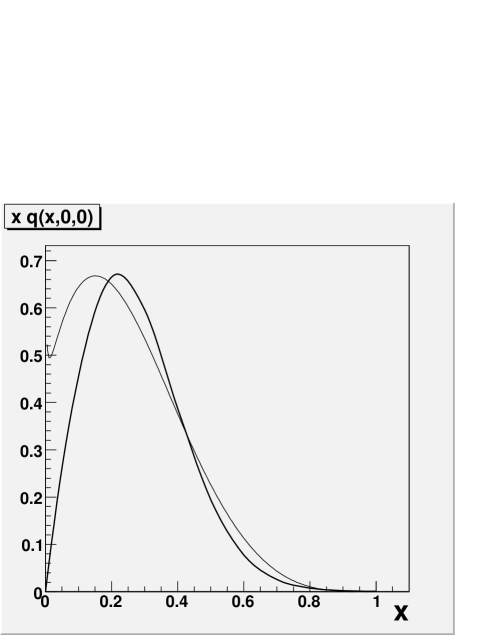
Figure 6: Unpolarized quark distribution: MRST[70] collinear distribution $xu(x)$ at $Q^{2}$ $=$ 16 GeV² and model $xq(x,k_{T}=0)$. The model curve is the one that tends to zero at small $x$.

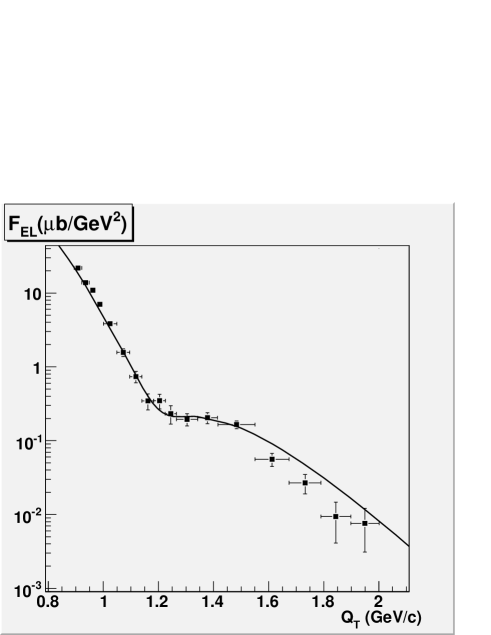
Figure 7: Fit of elastic $pp$ scattering data. $F_{EL}$ $\equiv$ $d\sigma/dt$. Data come from ref.[84].

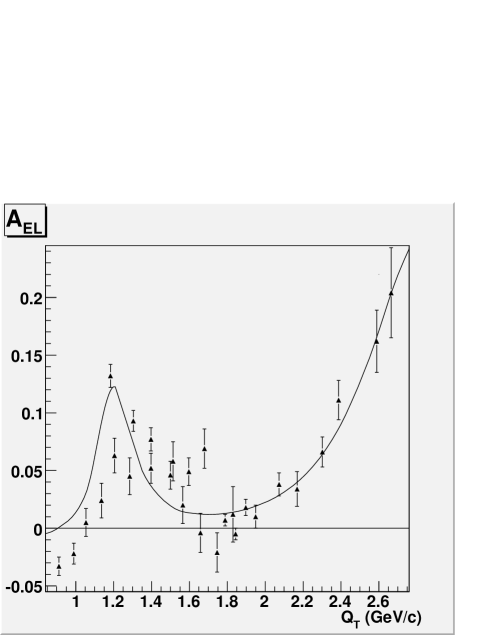
Figure 8: Fit of the analyzing power in elastic pp data. $A_{EL}$ $\equiv$ $[F_{EL}(k_{x})-F_{EL}(-k_{x})]/[F_{EL}(k_{x})+F_{EL}(-k_{x})]$. Data come from refs.[44, 45, 46, 47, 48].

4 Fit of scalar and spin-orbit interaction terms.

For extracting the distortion factor eq.24 from eq.25 applied to proton-proton elastic scattering, I have assumed that the projectile hadron participates to both processes (SIDIS or elastic scattering) with the same quark “intrinsic” distribution amplitude eq.19.

The phenomenology of normal spin observables in proton-proton scattering at 20-50 GeV, and $Q_{T}$ $=$ 1$-$3 GeV/c, is not trivial. Whichever the model, more analogous terms must be summed to reproduce it. Indeed, data show interference between at least two competing terms in elastic scattering[84, 43], and three competing terms in single-polarization measurements[44, 45, 46, 47, 48].

Here I ignore the behavior of the analyzing power in the very soft region (where it is nonzero but small), and include two scalar complex terms, and two imaginary spin-orbit terms. According to the relations of the previous sections, in all the cases any of the interaction 2x2 terms contains an overall scalar factor of the form $(\beta_{R}+i\beta_{I})exp[-(b/\Delta b)^{2}]exp[-(\xi/\Delta\xi)^{2}]$, where $(\beta_{R}+i\beta_{I})$ is the strength parameter, $\Delta b$ the transverse range and $\delta\xi$ the longitudinal range.

Also, the parameters of the quark bound state in the projectile are relevant, since this state is convoluted with the target interaction operator in the relevant matrix elements. This state too contains a factor of the form $exp[-(b/\Delta b)^{2}]exp[-(\xi/\Delta\xi)^{2}]$, so we may speak of transverse radius and longitudinal range for the bound state.

As evident from eq.25 the data of figs.7 and 8 cannot give information on any of the longitudinal ranges, of the quark bound state or of the interaction terms. For the quark bound state this parameter is constrained by the comparison with collinear distribution functions[70] (fig.6).

I have taken the longitudinal range of the quark bound state equal to 4.5, and all the longitudinal ranges of the interaction terms equal between them and equal to $4.5/\sqrt{2}$. This means that for all densities we have $\rho_{i}(\xi)$ $=$ $|\phi(\xi)|^{2}$. In other words, the same longitudinal range is attributed to all the terms of interest here.

This longitudinal range has been fixed by the fit in fig.6 a first time by calculating the unpolarized distribution in absence of all rescattering terms. It has been fine-tuned a second time after including the leading soft scalar ISI term (see below). It has been tuned once again after the remaining ISI terms had been included, but with no effect.

Data in fig.7 reproduce $pp$ elastic scattering at beam energy 50 GeV, taken from ref.[84]. The fit curve in this figure shows the left/right-averaged $Q_{T}-$distribution, i.e. for each $Q_{T}-$value I report the average of the two values of the distribution corresponding to $Q_{T}=\pm|Q_{T}|$. After this average, spin-orbit terms have negligible effect on the fit.

So spin-orbit terms are constrained by the data in fig.8 only. This figure reports data points from several experiments measuring the proton-proton normal spin analyzing power at 20-30 GeV beam energy[44, 45, 46, 47, 48].

4.1 The soft scalar term.

In fig.7 two regions are evident: a soft and a semihard region, corresponding to $Q_{T}$ below and over 1.2 GeV/c. The region below 1 GeV/c is dominated by the soft scalar term.

There is an important constraint on this term. For forward scattering, (i) the ratio $\rho$ of the real to the imaginary part of the amplitude is measured and assumes values between $-5$ and $-30$ % (decreasing with energy) in the region 20-50 GeV[68, 43], (ii) we are in single scattering regime, and the use of a Born-1 approximation is justified. This fixes the ratio of the real to the imaginary part of the related interaction potential. Indeed,

$$A_{born,1}(Q=0)\ \propto\ \int\hat{V}(\xi,\vec{b})d\xi d^{2}b$$ (36)

and

$$V(\xi,\vec{b})\ \propto\ exp\bigg{(}\int_{-\infty}^{\xi}\hat{T}(\xi^{\prime},\vec{b})d\xi^{\prime}\bigg{)}-1\ \approx\ \int_{-\infty}^{\xi}\hat{T}(\xi^{\prime},\vec{b})d\xi^{\prime},$$ (37)

So, for the soft scalar term that dominates forward scattering, $\hat{T}(\xi,b)$ has the same phase as $\rho$.

I have taken $Re(T)/Im(T)$ $=$ $-0.2$ (averaging a decreasing trend in the range 20-50 GeV). In practice, this ratio has little influence on the following, I have just assumed this value to conform with the known part of the phenomenology.

Since the central data peak is due to peripheral events, I have assumed that the transverse range of the interaction is much larger than the transverse radius of the bound quark state. With this assumption, the strength and slope of the central peak fix at once the strength of the scalar soft interaction term and the transverse radius of the bound state of the projectile quark. The transverse radius of the bound state is 1 fm. The strength of the scalar soft term is reported below, together with the strength of all terms. The precise value of the transverse range of the soft term has no effect as far as it is much larger than the bound state radius. I have taken it equal to 4 fm, but with 3 or 7 fm things do not change.

More in general, for any interaction term the (transverse) integral of eq.25 is cut off by the shorter between the bound state transverse and the interaction transverse range. When there is a relevant difference between the magnitude of the two, the precise value of the larger is not relevant. It must however be remarked that this property does not transfer automatically to eq.26, because of the absence of the “$-1$” subtraction in that case. This is clearly a source of ambiguity. In the case of the soft term it is anyway licit to guess that it has little effect on the asymmetry of the inclusive distributions, because of its reduced range in $Q_{T}-$space.

4.2 The semihard scalar term.

The parameters of the semihard scalar interaction term are given by fitting unpolarized scattering data (fig.7) in the shoulder region at $Q_{T}$ $>$ 1 GeV/c, and by the need of obtaining a nonzero analyzing power at $Q_{T}$ $>$ 1 GeV/c (fig.8).

The real and imaginary parts of the semihard scalar term are assumed equal in modulus. The sign of the imaginary part corresponds to flux production, and the sign of the real part to repulsive interaction. The transverse range of this term is fixed to 0.45 fm by the shape of the data of fig.7 for $Q_{T}$ $>$ 1 GeV/c.

A qualitative consideration of this semihard scalar term suggest that it mimics, within a single channel formalism, the effect of double scattering terms with intermediate formation of large-mass states (see the related discussion in section III.3 and Appendix B).

For fitting purposes, a nonzero imaginary part is needed, with opposite sign with respect to the soft term, to reproduce the interference pattern at 1.2 GeV/c. A nonzero positive real part does the same, because of a similar interference with the real part of the soft term. Because of the real to imaginary ratio of the soft part, with these signs the real part of the semihard potential contributes to 20 percent of the interference effect in the dip region.

In presence of a zero imaginary part, one would require a much larger strength for the real part to reproduce the dip. This larger strength would not fit the region $Q_{T}$ $>$ 1.2 GeV/c. The same would happen for a negative real part: the imaginary part should be increased to compensate.

The major role of the real part is to interfere with the imaginary spin-orbit terms producing a nonzero analyzing power. So, the real constraint on the real part arrive from the joint fit of data of fig.7 and fig.8. In addition, the strengths of the real part of the semihard scalar term and of the hard spin-orbit term are not fully independent.

4.3 Spin-orbit terms

Analyzing power data present three characteristic regions, only two of which evident in fig.8: (i) a low but nonzero (positive) broad peak at very small $Q_{T}$ (not showed in fig.8, but visible e.g. in [44]); (ii) a peak between 1 and 1.8 GeV/c; (iii) a large increase over 1.8 GeV.

Here, I neglect the ultra-soft peak at small $Q_{T}$. I introduce two spin-orbit imaginary terms: a soft term, with the same density structure as the scalar soft term, and a hard term, with a very small transverse interaction range 0.16 fm. The interference between the former and the semihard scalar term (real part) produces the nonzero values in the region 1$-$1.8 GeV/c, while the interference between the latter and the semihard scalar term (real part) produces the large$-Q_{T}$ rise.

The strength parameter for the soft spin-orbit term has been tuned so to best reproduce those points that present the smallest error bars in the confused data set of the region 1$-$1.8 GeV/c.

The hard spin-orbit term is necessary to reproduce the increase of the analyzing power in the $Q_{T}$ $>$ 1.8 GeV/c region. In fig.8, some points at large $Q_{T}$ with large error bars have not been reported. If taken at their central value, they would suggest even larger analyzing powers than the fitted ones. In addition, my fitting curve decreases for $Q_{T}$ $>$ 3 GeV/c. The decrease is driven by the fall of the scalar semihard term interfering with the spin-orbit terms. But we do not know what happens to data at $Q_{T}$ $>$ 3 GeV/c.

The dip at 1.6$-$1.8 GeV/c is due to the fact that neither of the two introduced spin-orbit terms is strong there. I have $not$ introduced a semihard spin-orbit term with range 0.5 fm as for the scalar potential, since it would produce large analyzing powers at $Q_{T}$ $=$ 1.6$-$1.8 where we see small or even negative analyzing power. Some of the small-error points reported in the figure are born from measurements that were specifically dedicated to the region 1.6$-$1.8 GeV/c. They confirmed with little doubt that in this region the analyzing power is close to zero.

The other dip, at 1 GeV/c, is well measured, and is due to the cancellation between the real parts of the two scalar interactions. Then the imaginary spin-orbit soft term cannot interfere with anything. On the left of this dip my fitting curve produces a very small, negative, rather flat analyzing power that does not correspond to reality (see e.g. [44]). Data show an again positive, but smaller than 5 %, analyzing power in the most forward region $Q_{T}$ $<$ 0.5 GeV/c. So, an extra term would be needed to explain quasi-forward data. Because of the smallness of the effect, I have not cared data at $Q_{T}$ $<$ 1 GeV/c.

4.4 Parameter values

Bound state longitudinal range: $\Delta\xi$ $=$ 4.5.

Longitudinal range of all the density widths: $\Delta\xi$ $=$ 4.5/$\sqrt{2}$.

The transverse width is peculiar:

quark bound state: $\Delta b$ $=$ 1 fm.

soft scalar and soft spin-orbit interaction: $\Delta b$ $=$ 4 fm.

semihard scalar interaction: $\Delta b$ $=$ 0.45 fm.

hard spin-orbit interaction: $\Delta b$ $=$ 0.16 fm.

The strength parameters are:

soft scalar interaction: $\delta$ $=$ 0.07 (i-0.2).

semihard scalar interaction: $\delta$ $=$ 0.01 (1-i).

soft spin-orbit interaction: $\alpha$ $=$ 0.0004 i.

hard spin-orbit interaction: $\alpha$ $=$ 0.0001 i.

5 Estimate of effects in inclusive processes

5.1 Distributions and asymmetries at quark level

Fourier transforms have been calculated assuming $\vec{k}_{T}$ coinciding with $(k_{x},0)$.

Fig.9 shows the quark distribution for positive and negative $k_{x}$, for $x$ $=$ 0.3. The two curves of fig.9 may also be read as the distributions corresponding, in both cases for positive $k_{x}$, to a parent hadron with spin oriented as $\pm\hat{y}$. Their non-identity implies a Sivers-like asymmetry and a nonzero function $q_{S}(x,k_{T})$ according with eq.7: $q(x,\vec{k}_{T})$ $\equiv$ $q_{U}(x,k_{T})$ $+$ $(k_{x}/M)q_{S}(x,k_{T})$, for an unpolarized quark in a hadron with polarization along $+\hat{y}$. For opposite hadron polarization $(k_{x}/M)q_{S}$ is substituted by $-(k_{x}/M)q_{S}$ (see eq.7). The $q_{S}/q_{U}$ ratio extracted from the difference between the two curves in fig.9 is shown in fig.10 as a function of $k_{T}$.

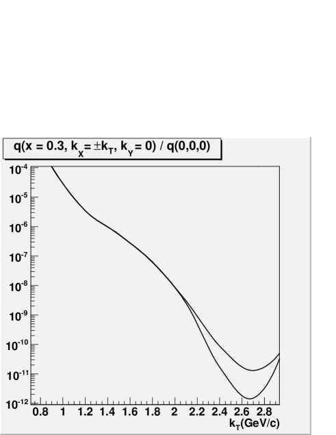
Figure 9: $k_{x}-$dependence for $x$ $=$ 0.3 and $k_{y}$ $=$ 0 of the quark distribution $q(x,k_{x},0)$ (see eq.7 in the text) for positive and negative $k_{x}$. These two curves refer to a parent proton polarized along $+\hat{y}$ and to an unpolarized quark. However, they also represent the positive $k_{x}$ distribution in the case of parent protons with opposite polarization $\pm\hat{y}$. The asymmetry between the shown curves is a Sivers-like asymmetry, from which the ratio between the Sivers and the unpolarized distribution may be extracted (next figure).

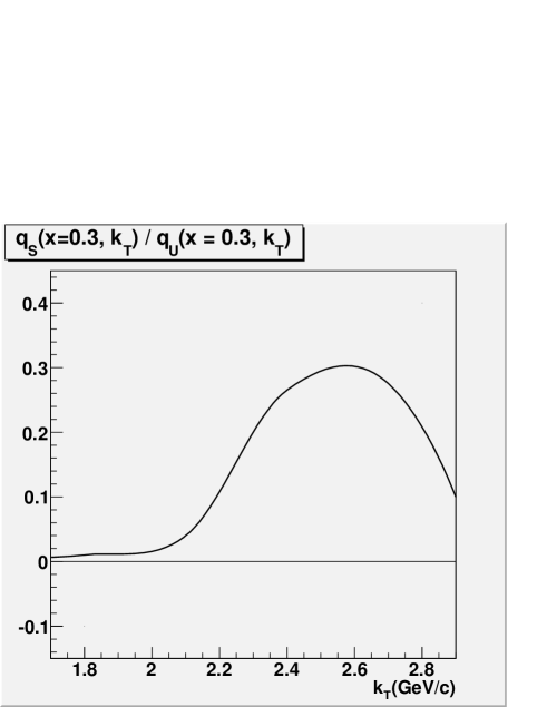
Figure 10: Ratio between the Sivers and the unpolarized distribution functions $q_{S}(x,k_{T})$ and $q_{U}(x,k_{T})$, as extracted from the asymmetry of the two curves reported in the previous figure (see eq.7 in the text). For $k_{T}$ $<$ 1.8 GeV/c the curve does not overcome 0.02.

Observations:

1) Figs 9 and 10 are completely representative of what may be seen at other values of $x$ in the valence region, e.g. $x$ $=$ 0.2.

2) Repeated application of the numerical calculation code shows that numerical calculations lose progressively reliability for $k_{T}$ $>$ 2.7 GeV/c at $x$ $=$ 0.3. For larger $x$ this loss of reliability is more severe, because of the fourier factor $exp(ix\xi)$. For this reason the value $x$ $=$ 0.3 has been chosen, as the largest $x$ value for which a reasonable $k_{x}-$range could be covered. For the same reason, $k_{y}$ has been fixed to zero.

Observing fig.9, although a flattening of the distribution at $k_{T}$ over 2 GeV/c is to be expected, the steep rise of the $k_{T}$ distribution at $k_{T}$ $\approx$ 3 GeV/c is not reliable. Up to 2.7 GeV/c the results of the numerical calculations are stable against changes of the integration point numbers and/or integration ranges. In the case of the figures referring to elastic scattering, stability arrives to 3 GeV/c.

3) The peak of the asymmetry evident at 2.4 GeV/c in fig.10, together with the disappearance of the asymmetry over 3 GeV/c, is not an effect of the code unreliability, but of the chosen interaction shapes. In other words, although numerical predictions are not reliable at 3 GeV/c, the fourier transform of the involved interaction terms must decrease in this region.

4) If one wants to compare the shape of the curves in figs. 9 and 10 with those in figs.7 and 8, one must observe that the transverse momentum scale of any phenomenon is slightly reduced in the quark distribution case. This is due to the fact that in eq.25 we find $|\psi(\xi,b)|^{2}$, while in in eq.26 we have $\psi(\xi,b)$. Because of the chosen gaussian shape, this means slightly harder effects in the elastic case.

5) Of the interaction terms inherited from elastic scattering, only the semihard and hard ones produces relevant effects on the quark distribution side. Soft scalar and spin-orbit terms are necessary to explain elastic data, but their effect on the asymmetry in the case of inclusive processes is small. In other words, the peak at 2.4 GeV/c in fig.10 can be reproduced after excluding all interaction terms but the quoted two. For $k_{T}$ $<$ 1.8 (not shown in fig.10) the asymmetry is never larger than about 0.2.

6) The fall of the asymmetry at small $k_{T}$ is an unavoidable consequence of the reduced size of the SSA in elastic scattering. For $k_{T}$ $>$ 3 GeV/c it is a consequence of the lack of hard interfering contributions, extracted from elastic scattering. It must be remarked, however, that in the case of large $k_{T}$ this lack is not constrained by elastic scattering data. Elastic scattering data do not show any decrease at large $k_{T}$. Simply, we do not know what happens for $k_{T}$ $>$ 3 GeV/c. But in fitting figs. 7 and 8 I have adopted a “minimal” approach, only introducing the strictly necessary interaction terms to reproduce the presently available data ranges. Both in the case of elastic and inclusive data this approach may lead to underestimation of asymmetries at large $k_{T}$.

7) Curves in figs. 8 and 10 present qualitative differences at intermediate $k_{T}$. This is due to two facts: (i) the presence of a fourier transform $exp(ix\xi)$ in the inclusive case, that changes the phase properties of the interaction terms, (ii) eq.26 does not contain the “$-1$” factor of eq.25, so in the inclusive case we have interference between no-rescattering and rescattering terms.

8) As specified in the Introduction, it is not possible to know whether the predicted effect is a leading twist or a higher twist one. So, if one names “Sivers function” the function $q_{S}(x,k_{T})$ that may be extracted from the asymmetry between the two curves of fig.9 using eq.7, the result shown in fig.10 may be read as a Sivers function in the sense that it $mimics$ a Sivers function at finite energies.

5.2 Convolution with a partner distribution

In all the relevant phenomenological cases, the calculated functions must be convoluted with a partner function $f(x^{\prime},\vec{k}_{T}^{\prime})$, so that the experimentally detected transverse momentum is $\vec{Q}_{T}$ $=$ $\vec{k}_{T}$ $+$ $\vec{k}_{T}^{\prime}$.

In a Drell-Yan event $f$ is the momentum distribution of an antiquark or of a gluon. In the case of meson production in hadron-hadron scattering, $f$ will be a convolution of distribution and fragmentation effects, so that $x^{\prime}$ and $\vec{k}_{T}^{\prime}$ will be product/sum of distribution and fragmentation variables. In both cases, we must distinguish the cases where $k_{T}^{\prime}$ derives from Fermi motion ($k_{T}^{\prime}$ $\approx$ 0-0.7 GeV/c) or from hard gluon secondary radiation ($k_{T}^{\prime}$ $>>$ 0.5 GeV/c).

The former one will be the case for $Q_{T}$ $<$ 3 GeV/c and for beam energies $<<$ 100 GeV. It is then realistic to imagine a gaussian distribution with pure Fermi motion origin like the following one:

$$f(x^{\prime},\vec{k}_{T}^{\prime})\ \propto\ e^{-(k_{T}/k_{0})^{2}}.$$ (38)

So, fig.11 in the following refers to this situation. For larger $Q_{T}$ and larger beam energies the requirement of a transverse momentum with dominating Fermi motion origin is not justified.

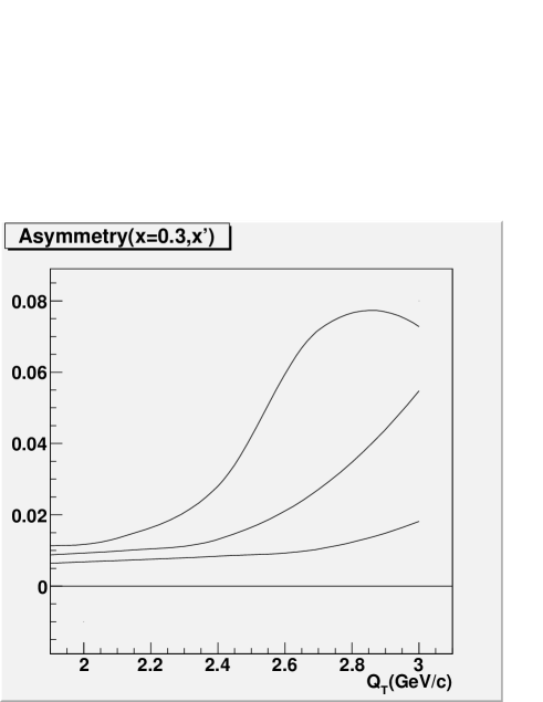
Figure 11: Estimate of a possible phenomenological asymmetry, e.g. in Drell-Yan or in meson production. Here the two quark distributions reported in fig.9 have been convoluted with a function $f(x^{\prime},\vec{k}_{T}^{\prime})$ $=$ $exp[-(k_{T}^{\prime}/k_{o})^{2}]f(x^{\prime})$ (see text), and $\vec{Q}_{T}$ $=$ $\vec{k}_{T}$ $+$ $\vec{k}_{T}^{\prime}$. The three curves correspond to $k_{o}$ $=$ 0.4, 0.5, 0.6 GeV/c (the asymmetry decreases for increasing $k_{o}$). The partner function $f(x^{\prime},\vec{k}_{T}^{\prime})$ may be the distribution function for an antiquark or gluon, or a combination of distribution and fragmentation effects, or also include recoil effects by radiation of undetected gluons. As evident, the asymmetry is visible if the momentum spread has Fermi motion origin ($k_{o}$ $<<$ 1 GeV/c) but not in the case where the momentum spread derives from gluon radiation ($k_{o}$ $>$ 1 GeV/c).

To correctly calculate a convolution for assigned $x$ and $x^{\prime}$, I need the values of $q(x,\vec{k}_{T})$ (the function appearing in eq.7 and plotted in fig.9) over a wide 2-dimensional range of $\vec{k}_{T}$. As previously observed, the numerical calculation of $q(x,\vec{k}_{T})$ is restricted by computational problems, that increase at increasing $k_{x}$ and $k_{y}$. For $x$ $=$ 0.3 and $k_{y}$ $=$ 0, I have a reliable set of values of $q(x,\vec{k}_{T})$ up to $k_{x}$ $=$ 2.6-2.8 GeV/c. To estimate a convolution, I make the simplifying hypothesis that $q(x,\pm\vec{k}_{T})$ depends on $k_{y}$ via a factorized term

$$q(x,\vec{k}_{T})\ =\ q(x,k_{x},0)q^{\prime}(k_{y}).$$ (39)

With this hypothesis, the terms that depend on $Q_{x}$ and $Q_{y}$ separate in the convolution $\int dk_{x}dk_{y}q(x,k_{x},k_{y})f(x^{\prime},Q_{x}-k_{x},Q_{y}-k_{y})$. For $Q_{y}$ $=$ 0, I simply obtain

$$\int dk_{x}dk_{y}\Big{[}q(x,k_{x},k_{y})f(x^{\prime},Q_{x}-k_{x},Q_{y}-k_{y})\Big{]}_{Q_{y}=0}\ =$$

$$=\ const\cdot\int dk_{x}q(x,k_{x},0)f(x^{\prime},0)e^{-[(Q_{x}-k_{x})/k_{0}]^{2}}$$ (40)

As for the calculation of fig.10, the above integral may be calculated for positive and negative $Q_{x}$. The corresponding asymmetry $(G_{+}-G_{-})/(G_{+}+G_{-})$ is shown in fig.11.

Obviously the asymmetry shown in fig.11 inherits the numerical uncertainties of the calculation of $q(x,\vec{k}_{T})$, and for this reason it cannot be considered 100 % reliable at the largest reported $Q_{T}$. As for fig.10, the qualitative origin of the asymmetry peak is the interference between semi-hard and hard interaction terms. The semi-hard term decreases for $k_{T}$ $>$ 2.5 GeV/c, and so indirectly for $Q_{T}$ $>$ 3 geV/c. So, qualitatively fig.11 shows nothing strange, but it cannot be considered precise for $Q_{T}$ $>$ 2.7 GeV/c.

Comparing fig.10 with fig.11 one notices that in the latter case we have a predictable spread of the asymmetry peak towards large $Q_{T}$, but not towards small $Q_{T}$. This is due to the steep decrease of the quark distribution $q(x,k_{x},0)$ (see fig.9) for $k_{x}$ $=$ 2$-$2.5 GeV/c. Events with $k_{x}$ $=$ 2.5 GeV/c and $k_{x}^{\prime}$ $=$ $-$0.5 GeV/c are much less frequent than events with $k_{x}$ $=$ 2 GeV and $k_{x}^{\prime}$ $=$ 0, so the former kind of events does not influence the region $Q_{x}$ $\approx$ 2 GeV/c.

For this reason, if the average $k_{T}^{\prime}-$spread of the partner distribution $f(x^{\prime},\vec{k}_{T}^{\prime})$ is increased from 0.4 GeV/c to larger values, the peak asymmetry decreases. So, the phenomenological effects are expected to depend in a marked way on the specific measurement.

Referring to the discussion in point (6) of subsection 5.1, it must be remarked that the fact that the found asymmetries decrease for $Q_{T}$ $<$ 2 GeV/c is a necessary consequence of the small (average) values of SSA in elastic scattering for $Q_{T}$ $<$ 1.8 GeV/c (fig.8). So, in the case of a relevant asymmetry (over 5 %) measured at $Q_{T}$ $<$ 1 GeV/c, I would exclude that it may have the origin that is described here.

On the contrary, there are no experimental constraints on the asymmetry values from elastic data at $Q_{T}$ $>$ 3 GeV/c, where more interaction terms could be present, aside of those considered here. I have adopted a “minimal” approach, in the sense of introducing just those interaction terms that are strictly necessary for reproducing the visible data. So the prediction reported here could underestimate asymmetries on the right side of the peak in figures 10 and 11.

5.3 Discussion

As previously observed, I do not imagine the term calculated by me to saturate the Sivers function. Rather, it is a contribution to it in a well-defined kinematic region. For the following discussion, I will name “AB-term” this contribution.

I will discuss the Drell-Yan application, since in this case we have some proved factorization statements[72, 73], a simple connection with the SIDIS (leptoproduction) case[8], absence of final state effects, a reference hard scale $Q$ (the dilepton mass) for $Q_{T}$, and a connection between the large-$Q_{T}$ and the small-$Q_{T}$ behavior of the Sivers asymmetry[11].

From figs. 10 and 11 it is evident that the AB-term may be relevant in the region $\Lambda$ $<<$ $Q_{T}$ $<<$ $Q$, for reasonable values of $Q$. $\Lambda$ may be any soft scale parameter. This region has been studied[11] because here the twist-3 model by refs.[12, 13] and the Sivers function scheme have overlapping regions of consistency. I name ”semihard $Q_{T}$ region” the above region.

The previous calculations refer to proton-proton collisions. As far as it can be considered scale-independent, the AB-term should be present in SIDIS too according with the change-of-sign rule stated in [8] for the leading-twist Sivers function.

In Drell-Yan we have two relevant scales: $Q$ and $Q_{T}$. It is normally admitted[6] that the Sivers asymmetry is power-suppressed in $Q_{T}$, but the associated Sivers function is anyway quoted as ”leading twist” if it is not power-suppressed with respect to $1/Q$ for fixed $x$ and $k_{T}$. Since $Q$ is related to the squared c.m. energy $s$ via the scaling variables $x_{1}$ and $x_{2}$ ($Q^{2}$ $=$ $x_{1}x_{2}s)$) “leading twist” means that in eq.7 $q_{S}$ depends on $s$ at most logarithmically (for fixed $x$ and $k_{T}$).

In this work $s$ is hidden in eq.21, in the dependence of $T^{\prime}$ on the momentum $k_{o}$ of the projectile quark (in a frame where the target hadron is at rest) This dependence means that the strength parameters $\delta_{n}$ and $\alpha_{n}$ in eqs. 31 and 34 are in principle functions of $s$. These parameters are extracted from the data in fig.7 and 8, so they can be considered as $s$-independent if these data do not depend on the beam energy. The data reported in fig.7 are stable for beam energy 20-50 GeV, and would show logarithmic changes at larger energies. Those of fig.8 are stable in the range 10-30 GeV, but we have no similar data at larger energies. So, I cannot presently establish whether the strength of the spin-orbit terms is $s$-independent or is not. If it is, the function shown in fig.10, with a change of sign, is a contribution to the Sivers function in leptoproduction.

If I decided to calculate directly (with a technique that is reasonably similar to the one adopted here) the SIDIS $\pi^{+}$ production on proton, this would be the crossed process of $\pi^{-}$-proton Drell-Yan. For the Sivers asymmetry in these two processes the calculation performed within my scheme would respect Collins’ rule (since the only change between the two cases would be in the integration path for the eikonal factor). However, the calculation of any of these two processes would require additional assumptions, since the elastic data of figs. 7 and 8 only constraint proton-proton ISI.

An obvious problem with figs. 10, 11 is the non regular rise of the asymmetry with respect to $Q_{T}$. A nonzero AB-term in the semihard region does not exclude the simultaneous presence of a Sivers function like those proposed in refs.[37, 38, 39, 40, 41, 42] filling the soft $Q_{T}$ region where the AB-term is small. Indeed, we may have mechanisms that are able to produce a single spin asymmetry in inclusive scattering but become ineffective, or effective but scarcely visible, when applied to elastic scattering. These mechanisms would escape the presented analysis.

On the other side, although nothing in my model forbids a nonzero AB-term at small $Q_{T}$, it is a matter of fact that, whatever mechanism produces a nonzero analyzing power in elastic scattering (data in fig.8), this mechanism has its top relevance in the region $Q_{T}$ $>$ 2 GeV/c, and rather small effects at $Q_{T}$ $<$ 1 GeV/c. So, to invent a model that transforms these small effects, observed in elastic scattering at small $Q_{T}$, into relevant effects in inclusive processes at the same $Q_{T}$ would not be trivial.

A over-simplified way to reproduce the physics described in this paper can be to imagine that, before the hard inclusive event, the two colliding protons scatter elastically and remain almost on shell up to the hard event. We know from the data of fig.8 that after the elastic scattering the space distribution of the colliding protons depends on the normal spin of the initial state. This is the entrance way to a nonzero Sivers asymmetry, since these protons enter the later hard scattering with asymmetric momentum distribution. The same data in fig.8 tell us that this effect is remarkable only when the $Q_{T}$ that is exchanged in the elastic scattering is semihard. We note that the effect is present also if quarks are completely collinear in the initial state, since what matters is the $Q_{T}$ exchanged in ISI. So one has a physical picture where the typical event characterized by a nonzero AB-term has small “primordial” $Q_{T}$, and a semihard $Q_{T}$ produced in ISI.

For the models of the Sivers asymmetry in Drell-Yan that are present in my reference list, we may distinguish two classes:

(A) models where the transverse momentum dependence of the cross section is entirely of Fermi motion, “primordial”, origin. Here $Q_{T}$ $=$ $k_{T1}$ $+$ $k_{T1}$ is the sum of the transverse momenta intrinsically associated with the distribution functions of the colliding quark and antiquark.

(B) models where the distribution functions are initially collinear, the $Q_{T}$-dependence of the cross section is associated with the hard nucleon-nucleon interaction (e.g. gluon radiation accompanying the hard vertex) and some arguments allow one to stick (part of) this effect to the individual quark distributions.

All the models extending the one by [7] belong to group A. The calculation in [11] belongs to group B. The model discussed here is mid-way between the two groups: the unperturbed quark distribution is narrow, but not fully collinear (it has a gaussian tail and transverse range 1 fm), and the event numbers at semihard $Q_{T}$ are strongly enhanced by ISI. The Glauber-Gribov approximation allows me to stick this enhancement to the quark distributions. In absence of ISI the curves in fig.9 would be lower in magnitude for $K_{T}$ over 1 GeV/c.

6 Conclusions

Summarizing, starting from the assumption that the quark total angular momentum is dominantly oriented as the parent hadron spin, it is possible to build a nonzero Sivers-like asymmetry via mean field initial state interactions of scalar and spin-orbit kind.

The specific form of the interactions, together with the values of the parameters, is here extracted from the phenomenology of proton-proton elastic scattering at 20-50 GeV. When these interactions are applied to transverse momentum dependent quark distributions, they produce an asymmetry that is important at transverse momenta 2-3 GeV/c, and reduces to very small values for smaller transverse momenta. It is not possible to estimate what happens over 3 GeV/c, for the lack of corresponding data in elastic proton-proton scattering.

With the present day knowledge of spin-orbit hadronic interactions, it is not possible to know whether their effects persist at very large energies. Consequently it is not possible to establish whether a Sivers-like asymmetry generated by them is a leading twist one or just an intermediate energy effect.

7 Appendix A

Solutions of the Dirac equation have in general four independent components. This is related with the existence of two solutions of the scalar equation $E^{2}=p^{2}+m^{2}$ and of two independent helicity states for each energy. In the two limiting cases

$$E\ \approx\ m\ +\ {p^{2}\over{2m}},$$ (41)

$$E\ \approx\ p_{z}\ +\ {m_{T}^{2}\over{2p_{z}}},$$ (42)

the structure simplifies. Although the use of a standard 4-component Dirac formalism may allow one to exploit a large set of well-known relations for trace calculation etc, it hides the fact that two components only are independent in the ultrarelativistic or nonrelativistic spinors.

Writing a 4-spinor in standard representation as

$$\Psi\ \equiv\ (\phi,\chi)$$ (43)

the two 2-spinors satisfy the coupled equations

$$\begin{array}[]{cc}(E-m)\phi\ =\ \vec{p}\cdot\ \vec{\sigma}\chi\\ (E+m)\chi\ =\ \vec{p}\cdot\ \vec{\sigma}\phi\\ \end{array}$$ (46)

equivalent to the Dirac equation.

We have the known nonrelativistic limit $\chi$ $\rightarrow$ 0 for particles, and the opposite limit for antiparticles. This decouples each other spin states, since the second one of eqs.46 loses relevance, and in the first one the right-hand side may be neglected. So, only interactions may remix spin states.

As well known, in the opposite limit $E$ $>>$ $m$ we have two relevant states $\phi\pm\chi$ that decouple each other. The nature of these states is clear after introducing helicity $\hat{n}\cdot\vec{\sigma}$. The u.r. limit may be reached for $E$ $\approx$ $\pm p_{z}$. For $E$ $\approx$ $+p_{z}$, $\phi+\chi$ coincides with one of the two helicity states, and $\phi-\chi$ with the other one. For $E$ $\approx$ $-p_{z}$, the correspondence is the opposite.

Instead of using helicity basis, I write the above equations 46 in terms of eigenstates of the spin projection along the $x-$axis $\phi_{x\pm}$ $\equiv$ $\phi_{T\pm}$:

$$\phi_{T-}\ =\ (1,1)/\sqrt{2},\hskip 14.22636pt\phi_{T-}\ =\ (1,-1)/\sqrt{2}$$ (47)

These 2-spinors satisfy the overlap relations

$$\begin{array}[]{cc}\sigma_{z}\phi_{T+}\ =\ \phi_{T-},\hskip 14.22636pt\sigma_{z}\phi_{T-}\ =\ \phi_{T+}\\ \sigma_{y}\phi_{T+}\ =\ -i\phi_{T-},\hskip 14.22636pt\sigma_{y}\phi_{T-}\ =\ i\phi_{T+}\end{array}$$ (50)

and the same for the corresponding $\chi_{T\pm}$ terms.

In the u.r. limit, from eq.46 one gets the relations

$$\phi_{T+}\ \approx\ \chi_{T-},\hskip 14.22636pt\phi_{T-}\ \approx\ \chi_{T+}$$ (51)

meaning that a spinor polarized along the transverse axis has the approximate form

$$\Psi_{T+}\ \equiv\ (\phi_{T+},\chi_{T+}),\ \approx\ (\phi_{T+},\phi_{T-}),\hskip 14.22636pt\Psi_{T-}\ \approx\ (\phi_{T-},\phi_{T+})$$ (52)

More precisely, in presence of a nonzero transverse momentum $p_{y}$ $<<$ $p_{z}$ that is also orthogonal to the normal spin, eqs.46 become (exploiting the previous eqs.50):

$$\begin{array}[]{cc}E\phi_{T+}-p_{z}\chi_{T-}\ +\ m\phi_{T+}+ip_{y}\chi_{T-}\ =\ 0,\\ E\chi_{T+}-p_{z}\chi_{T-}\ +\ m\phi_{T+}+ip_{y}\chi_{T-}\ =\ 0,\end{array}$$ (55)

so that $\phi_{T+}$ and $\chi_{T-}$ decouple from $\phi_{T-}$ and $\chi_{T+}$ (remark: $\phi_{T+}$ and $\chi_{T-}$ are pieces of different 4-spinors). Writing $E$ $=$ $(E-p_{z})$ $+$ $p_{z}$, the former of the previous two equations becomes

$$p_{z}(\phi_{T+}-\chi_{T-})\ +\ (E-p_{z})\phi_{T+}\ +\ m\phi_{T+}+ip_{y}\chi_{T-}\ =\ 0.$$ (56)

At $O(1/E)$ this confirms the equality between $\phi_{T+}$ and $\chi_{T-}$. Substituting $\chi_{T-}$ $=$ $\phi_{T+}$, and exploiting $E-p_{z}$ $\approx$ $m_{T}^{2}/2p$ $=$ $(m+ip_{y})(m-ip_{y})/2p$ one may also quantify the difference between the two spinors, that is $O(\phi_{T+}p_{y}/p_{z})$.

For the $\gamma_{+}$ projection we have (proportionality factors substitute powers of $1/\sqrt{2}$)

$$\Psi_{T+}^{+}\gamma_{0}\gamma_{+}\Psi_{T+}\ \propto\ \Psi_{T+}^{+}\left(\begin{array}[]{cc}1&\sigma_{z}\\ \sigma_{z}&1\end{array}\right)\Psi_{T+}\ =$$ (59)

$$\propto\ |\phi_{T+}|^{2}\ +\ \phi_{T+}^{+}\chi_{T-}\ +\ \chi_{T+}^{+}\phi_{T-}\ +\ |\chi_{T+}|^{2}\ \propto\ |\phi_{T+}|^{2}\ +\ |\phi_{T-}|^{2}.$$ (60)

and the same for $\Psi_{T-}$. In addition,

$$\Psi_{T+}^{+}\gamma_{0}\gamma_{+}\Psi_{T-}\ =\ \Psi_{T-}^{+}\gamma_{0}\gamma_{+}\Psi_{T+}\ =\ 0.$$ (61)

So, if a generic 4-spinor $\Psi$ has the form

$$\Psi\ \equiv\ \psi_{+}\Psi_{T+}\ +\ \psi_{-}\Psi_{T-}$$ (62)

we have, within corrections $O(1/E)$,

$$\bar{\Psi}\gamma_{+}\Psi\ \approx\ \Psi^{+}\gamma_{0}\gamma_{+}\Psi\ \approx\ |\psi_{+}|^{2}\ +\ |\psi_{-}|^{2},$$ (63)

i.e. the result exploited in eq.11 of the present work.

8 Appendix B

The exploitation of the Glauber technique in DWBA is better suited in nonrelativistic or ultrarelativistic form. In both limits it is often possible to approximate the kinetic energy in such a way that (i) a large part of the boost energy is removed from the problem, (ii) interactions may be inserted as additive contributions, to the zero or to the plus component of the energy-momentum vector. When (i) is true, the two treatments are equally effective. When it is not so, corrections are needed in both cases[83].

In the n.r. case, one normally uses a linearized Schroedinger equation, but relativistic kinematics. Since one always works with momenta, and interactions are directly fitted within this scheme, the hamiltonian is never involved and it is not surprising that this scheme may work in relativistic conditions. A detailed discussion of this and related references may be found in [80].

Limiting the discussion here to the scalar case for simplicity, in the n.r. case one of the possible starting points for the Glauber treatment is a linearized form of the Schroedinger equation, via the approximation

$$(k^{2}-\hat{p}^{2})\psi\ \approx\ 2k(k-\hat{p}_{z})\psi$$ (64)

where the kinetic energy is $(\hbar k)^{2}/2m$. Rescaling the potential energy as $2kV$ $\equiv$ $2mU/\hbar^{2}$ the linearized Schroedinger equation is

$$\hat{p}_{z}\psi\ =\ k(1+V)\psi,\hskip 14.22636ptV\ <<\ 1.$$ (65)

with stationary solution (for $V$ $<<$ 1)

$$\psi^{in}\ =\ exp\bigg{(}ikz+i\int_{-\infty}^{z}V(b,z^{\prime})dz^{\prime}\bigg{)},$$ (66)

that is the n.r. version of the wavefunction $\psi_{o}$ appearing in eq.23. The corresponding solution $\psi^{out}$ has $\int_{-\infty}^{z}$ substituted by $\int_{z}^{-\infty}$.

For the calculation of the matrix element $<\psi_{f}|\psi_{o}>$ in eq.23, the eikonal direction $\hat{z}$ of the dominating $exp(ikz)$ factor is rotated to $k\hat{z}\pm(q/2)\hat{x}$ in the initial or final wave, while the eikonal distortion factor is still approximately calculated along the direction $\hat{z}$ that is the average direction between the initial and final wave vectors.

For the insertion of the interactions in the u.r. case, there are different possibilities. The one adopted here is to insert the interaction $T$ into the u.r. equation

$$(xP_{+}\ -\ \hat{p}_{+})\psi\ \approx\ 0,$$ (67)

that becomes

$$(\hat{p}_{+}\ -\ xP_{+}\ +\ P_{+}T)\psi\ =\ 0.$$ (68)

When this equation is written in terms of the rescaled variable $\xi$ $=$ $P_{+}z_{-}$ we get the solution

$$\psi\ =\ exp\bigg{(}-ix\xi+i\int_{-\infty}^{\xi}T(b,\xi^{\prime})d\xi^{\prime}\bigg{)}$$ (69)

appearing in eq.23 (rotated $k\hat{z}$ $\rightarrow$ $k\hat{z}\pm(q/2)\hat{x}$).

Evidently, the previous u.r. and n.r. solutions are equivalent, once the interaction factors $V$ and $T$ are correctly related each other.

The tricky point[83] is that in both cases one assumes that some observable, associated with the longitudinal highly relativistic motion, is $constant$. In the n.r. case it is $k$, in the u.r. case, it is $x$. “Constant” means “conserved during all the development of the motion”. This way, the corresponding operator is substituted by its eigenvalue in the wave equation.

Multiple interactions may initially convert the initial quark state with mass $m$ into a more complex intermediate state with invariant mass $M$ (e.g., a quark plus a quark-antiquark pair). If this state is converted again into a single quark state, it contributes to elastic scattering. In highly relativistic conditions we have changes of $p_{z}$ (in intermediate states)

$$\Delta p_{z}\ \sim\ {{M^{2}-m^{2}}\over p_{z}},\hskip 14.22636ptM\ <\ M_{up}$$ (70)

where $M_{up}$ is a reasonable upper bound for the spectrum of intermediate states that may play some role.

The classical Glauber regime requires $M_{up}$ $<<$ $p_{z}$. In this case $p_{z}$ $\approx$ constant in the interactions, the $O(p_{z})$ term has no dynamical role, and the really relativistic part of the quark wavefunction disappears from the problem.

The Gribov regime is the one where in the limit $p_{z}$ $\rightarrow$ $\infty$, $M_{up}$ $=$ $\alpha p_{z}$ with small but nonzero $\alpha$. Then we have finite $O(\alpha)$ changes in $x$ during the intermediate stages of the process, invalidating the above assumption that $x$ is a constant of motion.

Since a full inclusion of inelastic channels is a difficult and unsolved problem, such channels are normally taken into account via two techniques: the first one is to introduce a discrete and limited set of intermediate non-elastic channels[87]. The other one is to rewrite the interaction terms in a non-hermitean form.

The latter treatment is $formally$ equivalent to a multi-channel treatment, as far as one is interested in the evolution of the elastic channel only. For nonrelativistic nuclear physics, this was demonstrated by Feshbach[82]. The scheme employed by him is quite abstract, and it can be generalized practically to any algebraic set of coupled equations describing the evolution of a state vector. So this equivalence may be considered general. The drawback of this generality is that it is practically impossible to use Feshbach’s arguments to calculate the form of the effective interaction from first principles.

So, in this work I had to guess a general form for the interaction operator $\hat{T}$, and fit it on elastic proton-proton scattering according to eq.25.

A last relevant point is that the treatment via the single channel effective potential does not transport the kinematics of the rescattering process out of the Glauber region (the price for this is that momenta are complex). Rescattering in the Glauber region does not create problems with factorization, at least in the Drell-Yan case for which an exhaustive discussion of the problem exists[72, 73].

References

References

- [1] PANDA collaboration, L.o.I. for the Proton-Antiproton Darmstadt Experiment (2004), http://www.gsi.de/documents/DOC-2004-Jan-115-1.pdf.
- [2] GSI-ASSIA Technical Proposal, Spokeperson: R.Bertini, http://www.gsi.de/documents/DOC-2004-Jan-152-1.ps;
- [3] P. Lenisa and F. Rathmann [for the PAX collaboration], hep-ex/0505054.
- [4] see e.g. G.Bunce, N.Saito, J.Soffer, and W.Vogelsang, Ann.Rev.Nucl.Part.Sci. 50 525 (2000) [arXiv:hep-ph/0007218].
- [5] R.Bertini, O.Yu Denisov et al, proposal in preparation.
- [6] D.Sivers, Phys.Rev. D41, 83 (1990); D.Sivers, Phys.Rev. D43, 261 (1991).
- [7] S.J.Brodsky, D.S.Hwang, and I.Schmidt Phys.Lett. B530, 99 (2002); S.J.Brodsky, D.S.Hwang, and I.Schmidt Nucl.Phys. B642, 344 (2002);
- [8] J.C.Collins, Phys.Lett. B536, 43 (2002);
- [9] X.-D.Ji and F.Yuan, Phys.Lett. B543, 66 (2002);
- [10] A.V.Belitsky, X.-D.Ji and F.Yuan, Nucl.Phys. B656, 165 (2003);
- [11] X.Ji, J.W.Qiu, W.Vogelsang and F.Yuan, Phys.Rev.Lett.97 082002 (2006); X.Ji, J.W.Qiu, W.Vogelsang and F.Yuan, Phys.Rev.D 73, 094017 (2006).
- [12] A.V.Efremov and O.V.Teryaev, Sov.J.Nucl.Phys. 36 140 (1982) [Yad. Fiz. 36 242 (1982)]; A.V.Efremov and O.V.Teryaev, Phys.Lett.B 150 383 (1985).
- [13] J.W.Qiu and G.Sterman, Phys.Rev.Lett.67 2264 (1991); J.W.Qiu and G.Sterman, Nucl.Phys.B 378 52 (1992); J.W.Qiu and G.Sterman, Phys.Rev.D 59 014004 (1999).
- [14] M.Anselmino et al, Phys.Rev.D72, 094007 (2005);
- [15] W.Vogelsang and F.Yuan, Phys.Rev.D72, 054028 (2005);
- [16] J.C. Collins, A.V. Efremov, K. Goeke, M. Grosse Perdekamp, S. Menzel, B. Meredith, A. Metz, and P.Schweitzer, Phys.Rev. D73 094023 (2006).
- [17] A.Bianconi and M.Radici, Phys.Rev. D 73 (2006) 034018.
- [18] M.Anselmino, M.Boglione, U.D’Alesio, A.Kotzinian, S.Melis, F.Murgia, A.Prokudin, and C.Turk, arXiv:0805.2677.
- [19] J.Adams et al (STAR), Phys.Rev.Lett. 92, 171801 (2004);
- [20] A.Airapetian et al (HERMES), Phys.Rev.Lett. 94, 012002 (2005);
- [21] V.Y.Alexakhin et al (COMPASS), Phys.Rev.Lett. 94, 202002 (2005);
- [22] S.S.Adler et al (PHENIX), Phys.Rev.Lett. 95, 202001 (2005);
- [23] New data from collaborations Hermes and Compass presented at the workshop “transversity 2008”, Ferrara, Italy, 28-31 may 2008, Proceedings in preparation.
- [24] P.V.Pobylitsa, hep-ph/0301236 (2003);
- [25] U.D’Alesio and F.Murgia Phys.Rev. D70 074009 (2004).
- [26] M.Burkardt, Nucl.Phys. A735, 185 (2004); M.Burkardt and D.S.Hwang, Phys.Rev. D69, 074032 (2004); M.Burkardt, Phys.Rev. D69, 057501 (2004).
- [27] A.Drago, Phys.Rev. D71, 057501 (2005).
- [28] A.Bianconi and M.Radici, J.Phys.G 31 645 (2005).
- [29] K. Goeke, S. Meissner, A. Metz, and M. Schlegel, Phys.Lett. B637 241 (2006).
- [30] D.Boer and W.Vogelsang Phys.Rev. D74 014004 (2006).
- [31] A.Bianconi and M.Radici, J.Phys.G 34 1595 (2007).
- [32] A.Bianconi, Phys.Rev.D 75, 074005 (2007).
- [33] Y.Koike, W.Vogelsang, and F.Yuan, arXiv:0711.0636, in press on Phys.Lett.B.
- [34] A.Bacchetta, M.Diehl, K.Goeke, A.Metz, P.J.Mulders, and M.Schlegel, JHEP 0702, 093 (2007).
- [35] A.Bacchetta, D.Boer, M.Diehl, and P.J.Mulders, arXiv:0803.0227.
- [36] R.Jakob, P.J.Mulders and J.Rodriguez, Nucl.Phys.A626 937 (1997).
- [37] D.Boer, S.J.Brodsky, and D.S.Hwang, Phys.Rev. D 67, 054003 (2003).
- [38] L.P.Gamberg, G.R.Goldstein, and K.A.Oganessyan Phys.Rev. D67, 071504(R) (2003).
- [39] A.Bacchetta, A.Schaefer, and J.-J.Yang, Phys.Lett. B578, 109 (2004).
- [40] Z.Lu and B.-Q.Ma, Nucl.Phys. A741, 200 (2004).
- [41] F.Yuan, Phys.Lett. B575, 45 (2003).
- [42] A.Courtoy, F.Fratini, S.Scopetta, and V.Vento, arXiv:0801.4347.
- [43] C.Lechanoine-LeLuc and F.Lehar, Rev.Mod.Phys. 65, 47 (1993).
- [44] D.G.Crabb et al, Phys.Rev.Lett.65, 3241 (1990).
- [45] P.R.Cameron et al, Phys.Rev. D 32, 3070 (1985).
- [46] D.C.Peaslee et al, Phys.Rev.Lett. 51, 2359 (1983).
- [47] P.H.Hansen et al, Phys.Rev.Lett. 50, 802 (1983).
- [48] J.Antille et al, Nucl. Phys. B 135 1 (1981).
- [49] G.R.Goldstein and M.J.Moravcsik, Ann. of Phys.142 219 (1982).
- [50] G.R.Goldstein and M.J.Moravcsik, Phys.Rev.D 32 303 (1985).
- [51] P.V.Landshoff and J.C.Polkinghorne, Nucl.Phys.B 32 541 (1971).
- [52] S.A.Gottlieb, D.Sivers and G.H.Thomas, Phys.Rev.D 20, 202 (1979).
- [53] G.R.Farrar, Phys.Rev.Lett.56, 1643 (1986).
- [54] S.J.Brodsky, C.E.Carlsson, and H.J.Lipkin Phys.Rev.D 20, 2278 (1979).
- [55] C.E.Bourrely, J.Soffer, and T.T.Wu, Phys.Rev.D 19, 3249 (1979); C.E.Bourrely, J.Soffer, and T.T.Wu, Nucl.Phys. B 247, 15 (1984); C.E.Bourrely, J.Soffer, Phys.Rev.D 35, 145 (1987).
- [56] P.A.Kazaks and D.L.Tucker, Phys.Rev.D 37, 222 (1988).
- [57] S.G.Brodsky and G.G.de Teramond, Phys.Rev.Lett. 60, 1924 (1988); S.G.Brodsky, I.Schmidt, and G.G.de Teramond, Phys.Rev.Lett. 64, 1011 (1990).
- [58] M.Anselmino, Z.Phys.C 13, 63 (1982).
- [59] H.J.Lipkin, Nature 324, 14 (1986); H.J.Lipkin, Phys.Lett.B 181, 164 (1987).
- [60] A.W.Hendry, Phys.Rev.D 10, 2300 (1974); A.W.Hendry, Phys.Rev.D 23, 2075 (1981);
- [61] J.P.Ralston and B.Pire, Phys.Rev.Lett.57, 2330 (1986).
- [62] Y.Tomozawa, Phys.Rev.D 36, 2854 (1987).
- [63] G.F.Wolters, Phys.Rev.Lett.45, 776 (1980).
- [64] L.Durand and F.Halzen Nucl.Phys.B 104, 317 (1976).
- [65] M.Sakamoto and S.Wakaizumi, Progr.Theor.Phys.62, 1293 (1979). S.Wakaizumi, Progr.Theor.Phys.67, 531 (1982).
- [66] C.Avilez, G.Cocho, and M.Moreno, Phys.Rev.D 24, 634 (1981).
- [67] C.E.Bourrely, Phys.Reports 177, 319 (1989).
- [68] G.Bellettini et al, Phys.Lett.14, 164 (1965).
- [69] R.J.Glauber, in “Lectures in Theoretical Physics”, edited by W.Brittain and L.G.Dunham (Interscience Publ., New York, 1959) Vol.1.
- [70] A.D.Martin, R.G.Roberts, W.S.Stirling, and R.S.Thorne, Eur.Phys.J.C 28 455; A.D.Martin, R.G.Roberts, W.S.Stirling, and R.S.Thorne, Eur.Phys.J.C 35 325;
- [71] HEPDATA: the Durham HEP Database, cared by the Durham Database Group of the Durham University (UK). http://durpdg.dur.ac.uk/
- [72] J.C.Collins, D.E.Soper and G.Sterman, Nucl.Phys. B261 104 (1985); J.C.Collins, D.E.Soper and G.Sterman, Nucl.Phys. B308 833 (19888).
- [73] G.Bodwin, Phys.Rev. D31 2616 (1985); G.Bodwin, Phys.Rev. D34 3932 (1986);
- [74] A.Bacchetta, U.d’Alesio, M.Diehl, and C.A.Miller, Phys.Rev.D 70 117504 (2004).
- [75] A.Bacchetta, Ph.D.Thesis, hep-ph/0212025.
- [76] P.J.Mulders, lectures given at the “International school on particle production spanning MeV and TeV physics”, Nijmegen, august 1999, hep-ph/9912493.
- [77] T.Henkes et al, Phys.Lett. B 283, 155 (1992).
- [78] V.V.Anisovich, M.N.Kobrinsky, J.Nyiri, and Yu.M.Shabelsky, “Quark model and high energy collisions”, World Scientific, Singapore, 1985.
- [79] N.N.Nikolaev, J.Speth, and B.G.Zakharov, J.Exp.Theor.Phys.82 1046 (1996).
- [80] A.Bianconi and M.Radici, Phys.Lett.B 363 24 (1995); A.Bianconi and M.Radici, Phys.Rev.C 53 563 (1996); A.Bianconi and M.Radici, Phys.Rev.C 54 3117 (1996);
- [81] A.Bianconi, S.Jeschonnek, N.N.Nikolaev, and B.G.Zakharov, Nucl.Phys.A 608 437 (1996). Erratum-Ibid.A 616 680.
- [82] H.Feshbach, Ann.Phys. 5 357 (1958). H.Feshbach, Ann.Phys. 19 287 (1962). A.K.Kerman, H.McManus, and R.M. Thaler, Ann.Phys. 8 551 (1959).
- [83] V.N.Gribov, ZhETF 56 892 (1969); Soviet Physics JETP 29 483 (1969).
- [84] Asad et al, Nuclear Physics B 255, 273 (1985).
- [85] J.C.Collins, Nucl.Phys.B 396, 161 (1993).
- [86] J.S.Conway et al, Phys.Rev.D 39, 92 (1989).
- [87] B.Z.Kopeliovich and L.I.Lapidus, Pis’ma ZhETF 28 664 (1978); JETP Lett. 28 614 (1978).