Prime pairs and zeta’s zeros

Abstract.

There is extensive numerical support for the prime-pair conjecture (PPC) of Hardy and Littlewood (1923) on the asymptotic behavior of $\pi_{2r}(x)$, the number of prime pairs $(p,\,p+2r)$ with $p\leq x$. However, it is still not known whether there are infinitely many prime pairs with given even difference! Using a strong hypothesis on (weighted) equidistribution of primes in arithmetic progressions, Goldston, Pintz and Yildirim have recently shown that there are infinitely many pairs of primes differing by at most sixteen. The present author uses a Tauberian approach to derive that the PPC is equivalent to specific boundary behavior of certain functions involving zeta’s complex zeros. Under Riemann’s Hypothesis (RH) and on the real axis these functions resemble pair-correlation expressions. A speculative extension of Montgomery’s classical work (1973) would imply that there must be an abundance of prime pairs.

1. Introduction

As of today, it is not known whether there are infinitely many prime twins $(p,\,p+2)$, or prime pairs $(p,\,p+2r)$ with given $r>0$. However, using a hypothesis on (weighted) equidistribution of primes in arithmetic progressions, Goldston, Pintz and Yildirim [20] have recently shown that there are infinitely many pairs of primes differing by at most sixteen; see also Goldston, Motohashi, Pintz and Yildirim [19] and the exposition by Soundararajan [36]. Let

$$\pi_{2r}(x)=\{\#\,\mbox{prime pairs}\;(p,\,p+2r)\;\mbox{with}\;p\leq x\}.$$

Around 1920 Viggo Brun used what is now called Brun’s sieve to prove that $\pi_{2}(x)=\mathcal{O}(x/\log^{2}x)$. In 1923 Hardy and Littlewood published a long paper [22] on the Goldbach problems and on prime pairs, prime triplets, etc. For prime pairs they conjectured the asymptotic formula

(1.1) $$\pi_{2r}(x)\sim 2C_{2r}{\rm li}_{2}(x)=2C_{2r}\int_{2}^{x}\frac{dt}{\log^{2}t}\sim 2C_{2r}\frac{x}{\log^{2}x}$$

as $x\to\infty$. Here

(1.2) $$C_{2}=\prod_{p\,{\rm prime},\,p>2}\,\left\{1-\frac{1}{(p-1)^{2}}\right\}\approx 0.6601618,$$

and

(1.3) $$C_{2r}=C_{2}\prod_{p|r,\,p>2}\,\frac{p-1}{p-2}.$$

Thus, for example, $C_{4}=C_{8}=C_{2}$, $C_{6}=2C_{2}$, $C_{10}=(4/3)C_{2}$. There is a great deal of numerical support for the prime-pair conjecture (PPC). On the Internet one finds counts of prime twins for $p$ up to $5\cdot 10^{15}$ by T. R. Nicely [33]. In Amsterdam Fokko van de Bult [4] has recently counted the prime pairs $(p,\,p+2r)$ with $2r\leq 10^{3}$ and $p\leq x=10^{3},\,10^{4},\,\cdots,\,10^{8}$. Table $1$ is based on his work. The bottom line shows (rounded) values $L_{2}(x)$ of the comparison function $2C_{2}{\rm li}_{2}(x)$. The table supports the conjecture that for every $r$ and $\varepsilon>0$

(1.4) $$\pi_{2r}(x)-2C_{2r}{\rm li}_{2}(x)\ll x^{(1/2)+\varepsilon}.$$

Here the symbol $\ll$ is shorthand for the $\mathcal{O}$-notation.

$2r\backslash x$	$10^{3}$	$10^{4}$	$10^{5}$	$10^{6}$	$10^{7}$	$10^{8}$	$C_{2r}/C_{2}$
2	35	205	1224	8169	58980	440312	1
4	41	203	1216	8144	58622	440258	1
6	74	411	2447	16386	117207	879908	2
8	38	208	1260	8242	59595	439908	1
10	51	270	1624	10934	78211	586811	4/3
12	70	404	2421	16378	117486	880196	2
14	48	245	1488	9878	70463	528095	6/5
16	39	200	1233	8210	58606	441055	1
18	74	417	2477	16451	117463	880444	2
20	48	269	1645	10972	78218	586267	4/3
22	41	226	1351	9171	65320	489085	10/9
24	79	404	2475	16343	117342	880927	2
30	99	536	3329	21990	156517	1173934	8/3
210	107	641	3928	26178	187731	1409150	16/5
$L_{2}(x)\,$:	46	214	1249	8248	58754	440368

Table 1. Counting prime pairs

Sieve methods have become an important part of prime-number theory. Using an advanced sieve, Jie Wu [41] has shown that $\pi_{2}(x)<6.8\,C_{2}\,x/\log^{2}x$ for all sufficiently large $x$. The best result in the other direction is J. R. Chen’s [8]: if $N(x)$ denotes the number of primes $p\leq x$ for which $p+2$ has at most two prime factors, then $N(x)\geq cx/\log^{2}x$ for some $c>0$. There are related results for prime pairs $(p,\,p+2r)$. In particular, for every $\varepsilon>0$ there is an $x_{0}=x_{0}(\varepsilon)$ independent of $r$ such that

(1.5) $$\pi_{2r}(x)\leq(8+\varepsilon)C_{2r}\,x/\log^{2}x\quad\mbox{for all}\;\;x\geq x_{0};$$

see the book Sieve Methods by Halberstam and Richert [21]. We will also use the fact that the prime-pair constants $C_{2r}$ have mean value one, for which Tenenbaum [37] has proposed an elegant proof. There is a strong estimate in the work of Bombieri and Davenport [3], which was sharpened by Friedlander and Goldston [10] to

(1.6) $$S_{m}=\sum_{r=1}^{m}C_{2r}=m-(1/2)\log m+\mathcal{O}\{\log^{2/3}(m+1)\}.$$

Starting with Montgomery’s work [31] one has realized that there is a deep connection between the prime-pair conjectures and the fine distribution of the complex zeros of the zeta function. Goldston in California has been an important contributor to the subject, cf. [18], [17]; several papers exploit the PPC to obtain plausible results on zeta’s zeros. Following a lead of Arenstorf [1] we will use a Wiener–Ikehara theorem to study prime pairs; the two-way form below is due to the author [28].

Theorem 1.1.

Let $\sum_{n=1}^{\infty}a_{n}/n^{w}$ with $a_{n}\geq 0$ converge to a sum function $f(w)$ for $w=u+iv$ with $u>1$. Then

(1.7) $$\sum_{n\leq x}\,a_{n}\,\sim\,Ax\quad\mbox{as}\;\;x\to\infty$$

if and only if for $u\searrow 1$, the difference

(1.8) $$f(u+iv)-\frac{A}{u+iv}=g(u+iv)$$

has a distributional limit $g(1+iv)$, which on every finite interval $(-B,B)$ coincides with a pseudofunction (that may a priori depend on $B$).

Ikehara [25] and Wiener [40] obtained (1.7) under the hypothesis that $g(w)$ has an analytic or continuous extension to the half-plane $\{u\geq 1\}$. The condition $\sum_{n\leq x}\,a_{n}=\mathcal{O}(x)$ would ensure that $f(u+iv)$ and $g(u+iv)$ have a distributional limit as $u\searrow 1$. A pseudofunction is the distributional Fourier transform of a bounded function which tends to zero at $\pm\infty$; locally, such a distribution is given by trigonometric series with coefficients that tend to zero. A pseudofunction cannot have pole-type singularities. In the case $a_{n}\geq 0$, local pseudofunction boundary behavior of $g(w)$ in (1.8) implies that

(1.9) $$(w-w_{0})g(w)\to 0$$

for angular approach of $w$ (from the right) to any point $w_{0}$ on the line $\{u=1\}$; cf. [26], or [27], Theorem III.3.1.

2. Basic auxiliary functions

For analytic formulation of the general PPC one may introduce the sums

$$\theta_{2r}(x)=\sum_{p,\,p+2r\,{\rm prime};\;p\leq x}\,\log^{2}p.$$

Relation (1.1) is equivalent to the asymptotic formula

$$\theta_{2r}(x)\sim 2C_{2r}x\quad\mbox{as}\;\;x\to\infty.$$

By the Wiener–Ikehara theorem this relation holds if and only if the function

$$\tilde{D}_{2r}(w)=\sum_{p,\,p+2r\,{\rm prime}}\,\frac{\log^{2}p}{p^{w}}$$

can be written as $2C_{2r}/(w-1)+g_{2r}(w)$, where $g_{2r}(w)$ has ‘good boundary behavior’ as $u\searrow 1$.

At this stage it is convenient to replace $\theta_{2r}(x)$ and $\tilde{D}_{2r}(w)$ by functions with similar behavior that involve von Mangoldt’s function $\Lambda(n)$. We recall its generating Dirichlet series; using the Euler product for $\zeta(w)$,

$$\sum_{n=1}^{\infty}\,\frac{\Lambda(n)}{n^{w}}=-\frac{\zeta^{\prime}(w)}{\zeta(w)}=\sum_{p\,{\rm prime}}\,(\log p)\bigg{(}\frac{1}{p^{w}}+\frac{1}{p^{2w}}+\cdots\bigg{)}.$$

One has $\Lambda(k)=\log p$ if $k=p^{\alpha}$ with $p$ prime, and $\Lambda(k)=0$ if $k$ is not a prime power. Since there are only $\mathcal{O}(\sqrt{x})$ prime powers $p^{\alpha}\leq x$ with $\alpha\geq 2$, the difference between

(2.1) $$\psi_{2r}(x)\stackrel{{\scriptstyle\mathrm{def}}}{{=}}\sum_{n\leq x}\,\Lambda(n)\Lambda(n+2r)$$

and $\theta_{2r}(x)$ is not much larger than $\sqrt{x}$. Thus the PPC is also equivalent to the relation

(2.2) $$\psi_{2r}(x)\sim 2C_{2r}x\quad\mbox{as}\;\;x\to\infty.$$

Similarly, the function

(2.3) $$D_{2r}(s)\stackrel{{\scriptstyle\mathrm{def}}}{{=}}\sum_{n=1}^{\infty}\,\frac{\Lambda(n)\Lambda(n+2r)}{n^{s}(n+2r)^{s}}\qquad(s=\sigma+i\tau,\,\sigma>1/2)$$

behaves in the same way as $\tilde{D}_{2r}(2s)$ when $2\sigma$ is close to $1$. Setting

(2.4) $$D_{2r}(s)-\frac{C_{2r}}{s-1/2}=G_{2r}(s),$$

the Wiener–Ikehara theorem with $2s$ instead of $w$ shows that the PPC (2.2) is equivalent to good boundary behavior of $G_{2r}(s)$ as $\sigma\searrow 1/2$.

Combinations. In order to profit from the fact that the constants $C_{2r}$ have mean value $1$ it helps to study sums $\sum_{2r\leq\lambda}\,D_{2r}(s)$ for large values of $\lambda$. Indeed, under the PPC, their boundary behavior should be roughly like that of $(\lambda/2)/(s-1/2)$. In this spirit we will study manageable combinations $V^{\lambda}(s)$ of functions $D_{2r}(s)$ with nonnegative coefficients. They are derived from a certain repeated complex integral $T^{\lambda}(s)$ (see Section 5) which extends and modifies an integral of Arenstorf [1]. It involves a parameter $\lambda>0$ and a parameter function $E^{\lambda}$; the resulting formula for $V^{\lambda}(s)$ is

(2.5) $$V^{\lambda}(s)\stackrel{{\scriptstyle\mathrm{def}}}{{=}}2\sum_{0<2r\leq\lambda}\,E^{\lambda}(2r)D_{2r}(s)=T^{\lambda}(s)-D_{0}(s)+H^{\lambda}(s).$$

Here the function $D_{2r}(s)$ is given by (2.3), also when $r=0$, and $H^{\lambda}(s)$ is holomorphic for $\sigma>0$. The parametric function $E^{\lambda}(\nu)=E(\nu/\lambda)$ acts as a sieving device. The basic function $E(\nu)$ is taken even, with compact support, Lipschitz continuous and decreasing on $[0,\infty)$. For convenience $E(\nu)$ is normalized so that its support is $[-1,1]$ and $E(0)=1$. The simplest sieving function $E^{\lambda}(\nu)$ is given by the Fourier transform of the Fejér kernel for ${\mathbb{R}}$,

$$E^{\lambda}_{F}(\nu)=\frac{1}{\pi}\int_{0}^{\infty}\frac{\sin^{2}(\lambda t/2)}{\lambda(t/2)^{2}}\cos\nu t\,dt=\left\{\begin{array}[]{ll}1-|\nu|/\lambda&\mbox{for $|\nu|\leq\lambda$,}\\ 0&\mbox{for $|\nu|\geq\lambda$.}\end{array}\right.$$

This function is adequate if one is willing to use Riemann’s Hypothesis (RH) in the proof of the main theorem; cf. the manuscript [29]. In the present paper we will prove the main result without appealing to RH, but for that have to require that $E$ be sufficiently smooth. More precisely, we suppose that $E$, $E^{\prime}$ and $E^{\prime\prime}$ are absolutely continuous with $E^{\prime\prime\prime}$ of bounded variation. One could for example use the Fourier transform of the Jackson kernel for ${\mathbb{R}}$,

$$E^{\lambda}_{J}(\nu) =\frac{3}{4\pi}\int_{0}^{\infty}\frac{\sin^{4}(\lambda t/4)}{\lambda^{3}(t/4)^{4}}\cos\nu t\,dt$$

(2.9) $$=\left\{\begin{array}[]{ll}1-6(\nu/\lambda)^{2}+6(|\nu|/\lambda)^{3}&\mbox{for $|\nu|\leq\lambda/2$},\\ 2(1-|\nu|/\lambda)^{3}&\mbox{for $\lambda/2\leq|\nu|\leq\lambda$},\\ 0&\mbox{for $|\nu|\geq\lambda$.}\end{array}\right.$$

The PPC and the mean value $1$ of the constants $C_{2r}$ lead one to expect that for large $\lambda$, $V^{\lambda}(s)$ has a first-order pole at $s=1/2$ with residue

(2.10) $$2\sum_{0<2r\leq\lambda}\,E(2r/\lambda)C_{2r}\approx\lambda\int_{0}^{1}E(\nu)d\nu\stackrel{{\scriptstyle\mathrm{def}}}{{=}}A^{E}\lambda.$$

For the following we need a Mellin transform associated with the Fourier transform of the kernel $E^{\lambda}$:

(2.11) $$M^{\lambda}(z)=M^{\lambda}_{E}(z)\stackrel{{\scriptstyle\mathrm{def}}}{{=}}\frac{1}{\pi}\int_{0}^{\infty}\hat{E}^{\lambda}(t)t^{-z}dt,\quad-1<x={\rm Re}\,z<1.$$

Proposition 2.1.

For our smooth $E$, the Mellin transform has a meromorphic extension to the half-plane $\{x>-3\}$, given by

(2.12) $$M^{\lambda}(z)=\frac{2}{\pi}\lambda^{z}\Gamma(-z-3)\sin(\pi z/2)\int_{0}^{1+}\nu^{z+3}dE^{\prime\prime\prime}(\nu)=\lambda^{z}M(z),$$

say. It has poles (of the first order) at $z=1,\,3,\,\cdots$. The residue at $z=1$ is $-(2\lambda/\pi)A^{E}=-(2\lambda/\pi)\int_{0}^{1}E(\nu)d\nu$ and $M^{\lambda}(0)=1$. For fixed $\lambda$ and any constant $C$ one has the majorization

(2.13) $$M^{\lambda}(x+iy)\ll(|y|+1)^{-x-7/2}\quad\mbox{for}\;\;-3<x\leq C,\;\;|y|\geq 1.$$

Proof.

The Fourier transform $\hat{E}^{\lambda}(t)$ is $\mathcal{O}\{(|t|+1)^{-2}\}$. By (2.11), initially taking $0<x<1$ and using the Mellin transform of $\cos\nu t$, cf. Section 4,

$$M^{\lambda}(z) =\frac{1}{\pi}\int_{0}^{\infty}t^{-z}dt\cdot 2\int_{0}^{\lambda}E^{\lambda}(\nu)(\cos t\nu)d\nu$$

$$=\frac{2}{\pi}\int_{0}^{\lambda}E^{\lambda}(\nu)d\nu\int_{0}^{\infty-}(\cos\nu t)t^{-z}dt$$

$$=\frac{2}{\pi}\Gamma(1-z)\cos\{\pi(1-z)/2\}\int_{0}^{\lambda}E^{\lambda}(\nu)\nu^{z-1}d\nu$$

$$=\frac{2}{\pi}\lambda^{z}\Gamma(1-z)\sin(\pi z/2)\int_{0}^{1}E(\nu)\nu^{z-1}d\nu.$$

For $x>0$ and smooth $E$, the final integral may also be written as

$$-\frac{1}{z}\int_{0}^{1}\nu^{z}dE(\nu) =\frac{1}{z(z+1)}\int_{0}^{1}\nu^{z+1}dE^{\prime}(\nu)$$

$$=\frac{1}{z(z+1)(z+2)(z+3)}\int_{0}^{1+}\nu^{z+3}dE^{\prime\prime\prime}(\nu).$$

This is enough to prove (2.12), hence $M^{\lambda}(z)$ has a meromorphic extension to the half-plane $\{x>-3\}$. The poles of $\Gamma(-z-3)$ at $z=-2,\,0,\,2,\,\cdots$ are cancelled by zeros of $\sin(\pi z/2)$ and the pole at $z=-1$ is cancelled by the zero of $\int_{0}^{1}\nu^{z+1}dE^{\prime}(\nu)$ at that point. The formulas also show that $M^{\lambda}(0)=1$ and that the residue at the pole $z=1$ is equal to $-(2\lambda/\pi)\int_{0}^{1}E(\nu)d\nu$. The order estimate (2.13) follows from the standard inequalities

(2.14) $$\Gamma(z)\ll|y|^{x-1/2}e^{-\pi|y|/2},\quad\sin(\pi z/2)\ll e^{\pi|y|/2}$$

which are valid for $|x|\leq C$ and $|y|\geq 1$. The inequality for $\Gamma(z)$ follows from Stirling’s formula for complex $z$; see formula (8.3) below. ∎

3. Results

Our results involve the complex zeros $\rho$ of the zeta function. Taking multiplicities into account, the zeros above the real axis will be arranged according to non-decreasing imaginary part:

$$\rho=\rho_{n}=\beta_{n}+i\gamma_{n},\;\;0<\gamma_{1}\approx 14<\gamma_{2}\approx 21\leq\cdots,\;\;n=1,\,2,\,\cdots$$

(with $\beta_{n}=1/2$ as far as zeros have been computed); we write $\overline{\rho}_{n}=\rho_{-n}$. The theorem below involves the sum

$$\Sigma^{\lambda}(s)\stackrel{{\scriptstyle\mathrm{def}}}{{=}}\left\{\frac{\zeta^{\prime}(s)}{\zeta(s)}\right\}^{2}$$

(3.1) $$\quad+2\,\frac{\zeta^{\prime}(s)}{\zeta(s)}\,\sum_{\rho}\,\Gamma(\rho-s)M^{\lambda}(\rho-s)\cos\{\pi(\rho-s)/2\}$$

$$+\sum_{\rho,\,\rho^{\prime}}\,\Gamma(\rho-s)\Gamma(\rho^{\prime}-s)M^{\lambda}(\rho+\rho^{\prime}-2s)\cos\{\pi(\rho-\rho^{\prime})/2\},$$

where $M^{\lambda}(\cdot)$ is given by (2.11). It is convenient to denote the sum of the first two terms by $\Sigma^{\lambda}_{1}(s)$ and to set the double sum equal to $\Sigma^{\lambda}_{2}(s)$. Results from Section 2 show that $\Sigma^{\lambda}_{1}(s)$ defines a meromorphic function for $\sigma<3$ whose only poles in the strip $\{0<\sigma<1\}$ occur at the complex zeros of $\zeta(\cdot)$. Under RH the double series, in which $\rho$ and $\rho^{\prime}$ both run over zeta’s complex zeros, is absolutely convergent for $1/2<\sigma<1$; cf. Lemma 4.2 below. Without RH the double sum may be interpreted as a limit of sums over the zeros $\rho$, $\rho^{\prime}$ with $|{\rm Im}\,\rho|$, $|{\rm Im}\,\rho^{\prime}|<R$; it will follow from Theorem 3.1 that the combination $\Sigma^{\lambda}(s)$ is in any case holomorphic for $1/2<\sigma<1$.

The formula for $V^{\lambda}(s)$ in (2.5) contains the function $T^{\lambda}(s)$ for which a repeated complex integral is introduced in Section 5. Moving the paths of integration in this integral and using the residue theorem one obtains

Theorem 3.1.

For any $\lambda>0$, any smooth sieving function $E$, and for $s=\sigma+i\tau$ with $1/2<\sigma<1$ there are holomorphic representations

$$V^{\lambda}(s) =2\sum_{0<2r\leq\lambda}\,E(2r/\lambda)D_{2r}(s)$$

(3.2) $$=\frac{-1/4}{(s-1/2)^{2}}+\frac{A^{E}\lambda}{s-1/2}+\Sigma^{\lambda}(s)+H^{\lambda}(s)$$

$$=\frac{A^{E}(\lambda-1)}{s-1/2}+\Sigma^{\lambda}(s)-\Sigma^{1}(s)+H^{\lambda}(s),$$

where $A^{E}=\int_{0}^{1}E(\nu)d\nu$ and $\Sigma^{\lambda}(s)$ is given by $(\ref{eq:3.1})$ (with proper interpretation of the double sum); the various functions $H^{\lambda}(s)$ are analytic for $1/2\leq\sigma<1$, and for $1/4<\sigma<1$ under RH. On the interval $\{1/2\leq s\leq 3/4\}$ one has $H^{\lambda}(s)=\mathcal{O}(\lambda\log\lambda)$ as $\lambda\to\infty$.

The (extended) Wiener–Ikehara Theorem will now show that the Hardy–Littlewood conjectures for prime pairs $(p,\,p+2r)$ are true if and only if the differences $\Sigma^{\lambda}(s)-\Sigma^{1}(s)$ exhibit certain specific boundary behavior as $\sigma\searrow 1/2$; cf. (2.4). To make this precise, define

(3.3) $$R(\lambda)=2\sum_{0<2r\leq\lambda}\,E(2r/\lambda)C_{2r}-A^{E}(\lambda-1).$$

By induction Theorems 3.1 and 1.1 imply

Corollary 3.2.

Suppose that the prime-pair conjecture for pairs $(p,\,p+2r)$ is true for every $r<m$. Then the PPC for prime pairs $(p,\,p+2m)$ is true if and only if for some (or every) smooth function $E$ and some (or every) number $\lambda\in(2m,2m+2]$, the function

(3.4) $$G^{\lambda}(s)\stackrel{{\scriptstyle\mathrm{def}}}{{=}}\Sigma^{\lambda}(s)-\Sigma^{1}(s)-\frac{R(\lambda)}{s-1/2}$$

has good (local pseudofunction) boundary behavior as $\sigma\searrow 1/2$.

The double series in (3) defines $\Sigma^{\lambda}_{2}(s)$ as a meromorphic function for $1/2<\sigma<1$ whose poles occur at complex zeros of $\zeta(\cdot)$, and these poles are cancelled by those of $\Sigma^{\lambda}_{1}(s)$. Formally there is cancellation also at the other complex zeros of $\zeta(\cdot)$. Turning to the function $G^{\lambda}(s)$, note that by (3.1), it does have good boundary behavior when $\lambda\leq 2$; under RH, it will even be analytic for $1/4<\sigma<1$. Indeed, $V^{\lambda}(s)=0$ for $\lambda\leq 2$. These observations support the following

Conjecture 3.3.

For every $\lambda>0$ and every $E$, the function $G^{\lambda}(s)$ in $(\ref{eq:3.4})$ has an analytic continuation to the strip $\{1/4<\sigma<1\}$.

If this is true, the counting functions $\pi_{2r}(x)$ all satisfy estimates of type (1.4).

Conditional abundance of prime pairs. It will follow from Section 7 that the part of the sum $\Sigma^{\lambda}_{2}(s)$ in which ${\rm Im}\,\rho$ and ${\rm Im}\,\rho^{\prime}$ have the same sign defines a meromorphic function for $1/2\leq\sigma<1$ whose only poles occur at complex zeros of $\zeta(\cdot)$. Thus for a study of its pole-type behavior near the point $s=1/2$, the double sum $\Sigma^{\lambda}_{2}(s)$ in (3) may be reduced to the sum $\Sigma^{\lambda}_{3}(s)$ in which ${\rm Im}\,\rho$ and ${\rm Im}\,\rho^{\prime}$ have opposite sign. Hence in the study of the PPC under RH, the differences of zeta’s zeros on the same side of the real axis play a key role.

Theorem 3.4.

Assume RH. Then the pole-type behavior of $\Sigma^{\lambda}_{3}(s)$ and $\Sigma^{\lambda}(s)$ as $s\searrow 1/2$ is the same as that of the reduced sum

(3.5) $$\Sigma^{\lambda}_{4}(s)=2\pi\sum_{\gamma,\,\gamma^{\prime};\,|\gamma^{\prime}-\gamma|<\gamma^{1/2}}\,\gamma^{-2s+i(\gamma-\gamma^{\prime})}M^{\lambda}\{1-2s+i(\gamma-\gamma^{\prime})\},$$

where $\gamma$ and $\gamma^{\prime}$ run over the imaginary parts of the zeros of $\zeta(\cdot)$ in the upper half-plane.

The expression in (3.5) is reminiscent of the pair-correlation function of zeta’s complex zeros which was studied by Montgomery [31] et al. Since the constants $C_{2r}$ have mean value $1$, the function $R(\lambda)$ in (3.3) is $o(\lambda)$ as $\lambda\to\infty$; cf. (2.10). [By (1.6) it will even be $\mathcal{O}(\log\lambda)$.] The corresponding hypothesis below regarding $\Sigma^{\lambda}(s)-\Sigma^{1}(s)$ would follow from a plausible extension of Montgomery’s work; see Section 9.

Hypothesis 3.5.

For smooth $E$ the ‘upper residue’

(3.6) $$\omega(\lambda)=\omega^{E}(\lambda)=\limsup_{s\searrow 1/2}\,(s-1/2)\{\Sigma^{\lambda}(s)-\Sigma^{1}(s)\}$$

is $o(\lambda)$ as $\lambda\to\infty$.

It follows from (3.1) and (1.5) that $\omega(\lambda)=\mathcal{O}(\lambda)$. If Hypothesis 3.5 is true there will be an abundance of prime pairs:

Theorem 3.6.

Assume Hypothesis 3.5. Then for every $\varepsilon>0$, there is a positive integer $m$, depending on $\omega(\cdot)$ and $\varepsilon$, such that

(3.7) $$\limsup_{x\to\infty}\,\frac{1}{m}\sum_{r\leq m}\,\frac{\pi_{2r}(x)}{x/\log^{2}x}>2-\varepsilon.$$

Here the constant $2$ would be optimal.

We finally mention an interesting positivity property of certain double sums $\Sigma^{\lambda}_{2}(s)$ in (3):

Proposition 3.7.

Let $E^{\lambda}$ be a sieving function (such as $E^{\lambda}_{J}$) for which $\hat{E}^{\lambda}(t)\geq 0$. Then $\Sigma^{\lambda}_{2}(s)\geq 0$ when $1/2<s<1$.

This positivity and a speculative equidistribution result for prime pairs with different values of $2r$ would also imply that there is an abundance of prime pairs; see Section 10.

4. Complex representation for $E^{\lambda}(\alpha-\beta)$

For the discussion of $T^{\lambda}(s)$ in Section 5 we need a complex integral for the sieving function $E^{\lambda}(\alpha-\beta)$ in which $\alpha$ and $\beta$ occur separately. It is obtained from the representation of $E^{\lambda}(\alpha-\beta)$ as an inverse Fourier (cosine) transform:

$$E^{\lambda}(\alpha-\beta)=\frac{1}{\pi}\int_{0}^{\infty}\hat{E}^{\lambda}(t)\cos\{(\alpha-\beta)t\}dt$$

and a repeated complex integral for

$$\cos\{(\alpha-\beta)t\}=\cos\alpha t\cos\beta t+\sin\alpha t\sin\beta t.$$

To set the stage we start with a complex representation for $\cos\alpha$ and $\sin\alpha$ with $\alpha>0$. Setting $z=x+iy$ we write $L(c)$ for the ‘vertical line’ $\{x=c\}$; the factor $1/(2\pi i)$ in complex integrals will be omitted. Thus

$$\int_{L(c)}f(z)dz\stackrel{{\scriptstyle\mathrm{def}}}{{=}}\frac{1}{2\pi i}\int_{c-i\infty}^{c+i\infty}f(z)dz.$$

Mellin inversion of the improper Euler integral

$$\int_{0}^{\infty-}(\cos\alpha)\alpha^{z-1}d\alpha=\Gamma(z)\cos(\pi z/2)\qquad(0<x<1)$$

now gives the improper complex integral

$$\cos\alpha =\int_{L(c)}^{*}\Gamma(z)\alpha^{-z}\cos(\pi z/2)dz$$

$$=\lim_{A\to\infty}\frac{1}{2\pi i}\int_{c-iA}^{c+iA}\,\cdots\quad(0<c<1/2);$$

there is a similar representation for $\sin\alpha$. It is important for us to have absolutely convergent integrals. We therefore replace the line $L(c)$ by a path $L(c,B)=L(c_{1},c_{2},B)$ with suitable $c_{1}<c_{2}$ and $B>0$ (cf. Figure 1):

(4.1) $$L(c,B)=\left\{\begin{array}[]{lllll}\mbox{$\quad$the half-line}&\mbox{$\{x=c_{1},\,-\infty<y\leq-B\}$}\\ \mbox{$+\;$the segment}&\mbox{$\{c_{1}\leq x\leq c_{2},\,y=-B\}$}\\ \mbox{$+\;$the segment}&\mbox{$\{x=c_{2},\,-B\leq y\leq B\}$}\\ \mbox{$+\;$the segment}&\mbox{$\{c_{2}\geq x\geq c_{1},\,y=B\}$}\\ \mbox{$+\;$the half-line}&\mbox{$\{x=c_{1},\,B\leq y<\infty\}$.}\end{array}\right.$$

Taking $c_{1}<-1/2$, $c_{2}>0$ and using formula (2.14), one thus obtains the absolutely convergent repeated integral

$$\cos\{(\alpha-\beta)t\} =\int_{L(c,B)}\Gamma(z)\alpha^{-z}t^{-z}dz\,\cdot$$

$$\quad\cdot\int_{L(c,B)}\Gamma(w)\beta^{-w}t^{-w}\cos\{\pi(z-w)/2\}dw.$$

Multiplying both sides by $\hat{E}^{\lambda}(t)$, integrating over $\{0<t<\infty\}$, inverting order of integration and using formula (2.11) for $M^{\lambda}(\cdot)$, one obtains

Proposition 4.1.

Let $\alpha,\,\beta>0$, $-3/2<c_{1}<0<c_{2}<1/2$ and $B>0$. Then for smooth sieving functions $E^{\lambda}(\cdot)$ as in Section 2 one has the representation

$$E^{\lambda}(\alpha-\beta) =\int_{L(c,B)}\Gamma(z)\alpha^{-z}dz\int_{L(c,B)}\Gamma(w)\beta^{-w}\,\cdot$$

(4.2) $$\quad\cdot M^{\lambda}(z+w)\cos\{\pi(z-w)/2\}\,dw.$$

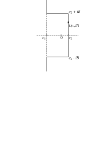
Figure 1. The path $L(c_{1},c_{2},B)$

To justify the operations and verify the absolute convergence of the integral in (4.1) one may use the estimate (2.13) and a simple lemma:

Lemma 4.2.

For real constants $a,\,b,\,c$, the function

$$\phi(y,v)=(|y|+1)^{-a}(|v|+1)^{-b}(|y+v|+1)^{-c}$$

is integrable over ${\mathbb{R}}^{2}$ if (and only if) $a+b>1$, $a+c>1$, $b+c>1$ and $a+b+c>2$. For integrability over ${\mathbb{R}}_{+}^{2}$ the condition $a+b>1$ may be dropped.

For verification let $A>0$. On the subset of ${\mathbb{R}}^{2}$ where $|y|\leq A$, the condition $b+c>1$ is necessary and sufficient for a finite $v$-integral. Similarly for $|v|\leq A$ and the condition $a+c>1$. When $|y+v|\leq A$ one needs the condition $a+b>1$ in the case of ${\mathbb{R}}^{2}$. For the fourth condition one looks at the set where $v\geq y\geq 1$. Setting $v=yr$ with new variable $r$,

$$\phi(y,v)dydv\asymp y^{-a}(yr)^{-b}\{y(r+1)\}^{-c}ydydr,$$

and the right-hand side is integrable over the set $\{1<y<\infty,\,1<r<\infty\}$ if and only if $b+c>1$ and $a+b+c>2$. Similarly when $y$ and $v$ have opposite sign; one may of course assume that $|y+v|>1$ then.

We turn to Proposition 4.1. Setting $z=x+iy$, $w=u+iv$, Stirling’s formula and (2.13) give the following majorant for the integrand in (4.1) on the remote parts of the paths $L(c,B)$:

$$(|y|+1)^{c_{1}-1/2}(|v|+1)^{c_{1}-1/2}(|y+v|+1)^{-2c_{1}-7/2}.$$

For integrability one thus needs $-3<c_{1}<0$. The more stringent requirements in the proposition serve to justify inversion of the order of integration in a triple integral and to keep the paths within the strip $\{-3<X<1\}$ where $M^{\lambda}(Z)$ is known to be regular.

5. The complex integral for $T^{\lambda}(s)$

The function $T^{\lambda}(s)$ in (2.5) is defined by the integral below for $\sigma>1+|c_{1}|$, while for $s$ with smaller real part it is defined by analytic continuation;

$$\quad T^{\lambda}(s) =\int_{L(c,B)}\Gamma(z)\frac{\zeta^{\prime}(z+s)}{\zeta(z+s)}\,dz\int_{L(c,B)}\Gamma(w)\frac{\zeta^{\prime}(w+s)}{\zeta(w+s)}\,\cdot$$

(5.1) $$\qquad\cdot M^{\lambda}(z+w)\cos\{\pi(z-w)/2\}dw.$$

Theorem 5.1.

Let $-3/2<c_{1}<0<c_{2}<1/2$. Then the integral $(\ref{eq:5.1})$ defines $T^{\lambda}(s)$ as a holomorphic function of $s=\sigma+i\tau$ for $\sigma>1-c_{1}$. Assuming RH, the integral gives $T^{\lambda}(s)$ as a holomorphic function for $\sigma>\max\{(1/2)-c_{1},1-c_{2}\}$ and $|\tau|<B$.

The integral has an analytic continuation to the half-plane $\{\sigma>1/2\}$ given by the expansion

(5.2) $$T^{\lambda}(s)=\sum_{k,l}\Lambda(k)\Lambda(l)k^{-s}l^{-s}E^{\lambda}(k-l).$$

Discussion.

For $z\in L(c,B)$ and $\sigma>1-c_{1}$, the sum $z+s$ will stay away from the poles of $\zeta^{\prime}/\zeta$. Under RH the same holds when $\sigma>\max\{(1/2)-c_{1},1-c_{2}\}$ and $|\tau|<B$. Indeed, in that case $x+\sigma>1/2$ and also $z+s\neq 1$: if $x+\sigma=1$, then $z$ must lie on the part of $L(c,B)$ where $|y|\geq B$, and then $y+\tau\neq 0$. Similarly for $w=u+iv$. The absolute convergence of the repeated integral in (5) can be proved in the same way as that of (4.1). Indeed, the quotient $(\zeta^{\prime}/\zeta)(Z)$ grows at most logarithmically in $Y$ for $X\geq 1$, and for $X\geq(1/2)+\eta$ under RH; cf. Titchmarsh [38]. The holomorphy of the integral for $T^{\lambda}(s)$ now follows from locally uniform convergence in $s$.

For the second part we substitute the Dirichlet series for $(\zeta^{\prime}/\zeta)(\cdot)$ into (5), initially taking $\sigma>1-c_{1}$. Integrating term by term and applying Proposition 4.1 one obtains the expansion (5.2). Because $E^{\lambda}(k-l)\neq 0$ only for finitely many values of $k-l$, the series represents a holomorphic function for $\sigma>1/2$; cf. the proof of Theorem 5.2 below. The sum of the series provides an (the) analytic continuation of the integral to the half-plane $\{\sigma>1/2\}$. ∎

We will now derive (2.5).

Theorem 5.2.

For arbitrary $\lambda>0$ and $\sigma>1/2$,

(5.3) $$T^{\lambda}(s)=D_{0}(s)+2\sum_{0<2r\leq\lambda}\,E(2r/\lambda)D_{2r}(s)+H^{\lambda}_{1}(s),$$

where $H^{\lambda}_{1}(s)$ is holomorphic for $\sigma>0$. On the real interval $\{1/2\leq s\leq 3/4\}$ one has $H^{\lambda}_{1}(s)=\mathcal{O}(\lambda)$ as $\lambda\to\infty$.

Proof.

Taking $k=l$ in (5.2) one obtains the term $D_{0}(s)$ in (5.3). For $|k-l|=2r$ one obtains a constant multiple of $D_{2r}(s)$. The coefficient is different from $0$ only if $2r<\lambda$ and in fact equal to $2E(2r/\lambda)$. If $|k-l|=2r-1$ one can have $\Lambda(k)\Lambda(l)\neq 0$ only if either $k$ or $l$ is of the form $2^{\alpha}$ for some $\alpha>0$. The resulting functions, for which $2r-1$ must be $<\lambda$, are holomorphic for $\sigma>0$. For real $s\searrow 1/2$ the sum $H^{\lambda}_{1}(s)$ of their values will be $\mathcal{O}(\lambda\log\lambda)$ as $\lambda\to\infty$. ∎

It remains to determine the analytic character of $D_{0}(s)$:

Lemma 5.3.

One has

(5.4) $$D_{0}(s)=\sum_{k=1}^{\infty}\,\frac{\Lambda^{2}(k)}{k^{2s}}=\frac{1/4}{(s-1/2)^{2}}+H_{0}(s),$$

where $H_{0}(s)$ is analytic for $\sigma\geq 1/2$, and for $\sigma>1/4$ under RH.

Indeed, for $x>1$

$$\sum_{k}\Lambda^{2}(k)k^{-z}=\sum_{p}(\log^{2}p)p^{-z}+H_{1}(z)=-\frac{d}{dz}\sum_{p}(\log p)p^{-z}+H_{1}(z)$$

$$=-\frac{d}{dz}\sum_{k}\Lambda(k)k^{-z}+H_{2}(z)=\frac{d}{dz}\frac{\zeta^{\prime}(z)}{\zeta(z)}+H_{2}(z)=\frac{1}{(z-1)^{2}}+H_{3}(z),$$

where $H_{1}(z)$ and $H_{2}(z)$ define holomorphic functions for $x>1/2$, while $H_{3}(z)$ is holomorphic for $x\geq 1$, and for $x>1/2$ under RH. Finally take $z=2s$.

6. Transformation of the integral for $T^{\lambda}(s)$

Taking $c_{1},\,c_{2}$ and $s$ as in the first part of Theorem 5.1 we will move the paths of integration in the integral for $T^{\lambda}(s)$, but first change variables. Replacing $z$ by $z^{\prime}-s$ and $w$ by $w^{\prime}-s$ (and subsequently dropping the primes), one obtains

$$T^{\lambda}(s) =\int_{L(c^{\prime},B^{\prime})}\Gamma(z-s)\frac{\zeta^{\prime}(z)}{\zeta(z)}\,dz\int_{L(c^{\prime},B^{\prime})}\Gamma(w-s)\frac{\zeta^{\prime}(w)}{\zeta(w)}\,\cdot$$

(6.1) $$\quad\;\cdot\,M^{\lambda}(z+w-2s)\cos\{\pi(z-w)/2\}dw.$$

Here the paths of integration will initially depend on $s$: $c^{\prime}_{1}=c_{1}+s$, $c^{\prime}_{2}=c_{2}+s$, and the horizontal segments may be at different distances from the real axis. However, by our standard estimates and Cauchy’s theorem, one may fix $c^{\prime}_{1}=1$ and $c^{\prime}_{2}=3/2$, say, use a constant $B^{\prime}$ and take $1<\sigma<3/2$, $|\tau|<B^{\prime}$. Observe that henceforth, the point $s$ will be to the left of the paths.

Starting with (6), where we rename $c^{\prime}_{1}=1=c_{1}$, $c^{\prime}_{2}=3/2=c_{2}$ and $B^{\prime}=B$, the paths of integration $L(c,B)$ will be moved across the poles $s$, $1$ and $\rho$ to the line $L(0)$, the imaginary axis. We first describe what happens when we move the $w$-path:

(6.2) $$T^{\lambda}(s)=\int_{L(c,B)}\cdots\,dz\int_{L(0)}\cdots\,dw+U^{\lambda}_{2}(s)=U^{\lambda}_{1}(s)+U^{\lambda}_{2}(s),$$

say, where by the residue theorem

(6.3) $$U^{\lambda}_{2}(s)=\int_{L(c,B)}\Gamma(z-s)\frac{\zeta^{\prime}(z)}{\zeta(z)}\,J(z,s)dz,$$

with

$$J(z,s) =\frac{\zeta^{\prime}(s)}{\zeta(s)}\,M^{\lambda}(z-s)\cos\{\pi(z-s)/2\}$$

(6.4) $$\quad-\Gamma(1-s)M^{\lambda}(z+1-2s)\cos\{\pi(z-1)/2\}$$

$$\quad+\sum_{\rho}\,\Gamma(\rho-s)M^{\lambda}(z+\rho-2s)\cos\{\pi(z-\rho)/2\}.$$

By the usual estimates and Lemma 4.2 the repeated integral $U^{\lambda}_{1}(s)$ defines a holomorphic function for $1/2<\sigma<3/2$, hence by Theorem 5.1, the function $U^{\lambda}_{2}(s)$ must have an analytic continuation to the same strip!

For $1<\sigma<3/2$ the function $J(z,s)$ is holomorphic in $z$ on and between the paths $L(c,B)$ and $L(0)$. If we define $J(z,s)$ for $z\in L(c,B)$ by continuity at $s=1$ and points $s=\rho$, it becomes holomorphic in $s$ for $3/4<\sigma<3/2$; apparent poles cancel each other. What can we say about the integral for $U^{\lambda}_{2}(s)$? The critical part is the one that corresponds to the sum over $\rho=\beta\pm i\gamma$ in (6). For $|y|>B\geq 2$ its integrand is majorized by

$$\sum_{\rho}|y|^{c_{1}-\sigma-1/2}(\log|y|)|\rho|^{\beta-\sigma-1/2}(|y+\rho|+1)^{-c_{1}-\beta+2\sigma-7/2}.$$

Since $c_{1}=1$, $0<\beta<1$ and $|\rho_{n}|\sim 2\pi n/\log n$ as $n\to\infty$, the analog of Lemma 4.2 for the integral of a sum proves the absolute convergence and holomorphy of the integral when $3/4<\sigma<3/2$.

To justify the above application of the residue theorem one may start with $w$-integrals over a sequence of closed contours $W_{R}$, $B<R=R_{k}\to\infty$, whose upper part is shown in Figure 2.

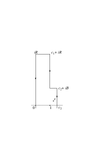
Figure 2. Upper half of $W_{R}$

Here the numbers $R=R_{k}$ are chosen ‘away from the numbers $\gamma_{n}$’, in the sense that on the horizontal segments $\{v=\pm R\}$ one has $\zeta^{\prime}(w)/\zeta(w)\ll\log^{2}|v|$. One may require that $R_{k}\in(k,k+1)$, $k=1,2,\cdots$; cf. the expansion of $(\zeta^{\prime}/\zeta)(\cdot)$ and ways of estimating this quotient in Titchmarsh [38]. One can now use the standard majorants to show that for $3/4<\sigma<3/2$,

$$\int_{L(c,B)}\Gamma(z-s)\frac{\zeta^{\prime}(z)}{\zeta(z)}\,dz\int_{c_{1}+iR}^{iR}\Gamma(w-s)\frac{\zeta^{\prime}(w)}{\zeta(w)}\,\cdot$$

(6.5) $$\quad\cdot\,M^{\lambda}(z+w-2s)\cos\{\pi(z-w)/2\}dw\to 0\quad\mbox{as}\;\;R\to\infty.$$

Similarly for the segment where $v=-R$. We summarize what we have found so far:

Proposition 6.1.

For $1<\sigma<3/2$ and $|\tau|<B$ the integral for $T^{\lambda}(s)$ admits a holomorphic decomposition $T^{\lambda}(s)=U^{\lambda}_{1}(s)+U^{\lambda}_{2}(s)$, see $(\ref{eq:6.2})$, in which both integrals $U^{\lambda}_{j}(s)$ define analytic functions for $3/4<\sigma<3/2$.

In a second step, inverting order of integration where necessary, the $z$-paths $L(c,B)$ in the integrals (6.2), (6.3) for $U^{\lambda}_{1}(s)$ and $U^{\lambda}_{2}(s)$ are moved to $L(0)$. Again using the residue theorem, this results in the decomposition

$$T^{\lambda}(s) =\int_{L(0)}\,\cdots\,dz\int_{L(0)}\,\cdots\,dw+2\int_{L(0)}\,\Gamma(z-s)\frac{\zeta^{\prime}(z)}{\zeta(z)}\,J(z,s)dz$$

(6.6) $$+\bigg{\{}\frac{\zeta^{\prime}(s)}{\zeta(s)}\,J(s,s)-\Gamma(1-s)J(1,s)+\sum_{\rho^{\prime}}\,\Gamma(\rho^{\prime}-s)J(\rho^{\prime},s)\bigg{\}}.$$

The new integrals will define holomorphic functions for $0<\sigma<1$. In the case of the single integral involving the sum over $\rho=\beta+i\gamma$ in $J(z,s)$, where $\beta$ might be close to $1$, this can be seen by moving the integral over to $L(-\eta)$ with variable $\eta\in(0,1)$. On the interval $\{1/2\leq s\leq 3/4\}$ the integrals are $\mathcal{O}(1)$ as $\lambda\to\infty$.

We now turn to the big residue in the last line of (6). With the aid of (6) it leads to nine terms. Four of these combine into the three terms of $\Sigma^{\lambda}(s)$ in (3); here the sum $\Sigma^{\lambda}_{2}(s)$ of the double series has to be formed in a suitable way as described below. Another term gives the important constituent

(6.7) $$U^{\lambda}_{3}(s)\stackrel{{\scriptstyle\mathrm{def}}}{{=}}\Gamma^{2}(1-s)M^{\lambda}(2-2s).$$

By Proposition 2.1 the function $U^{\lambda}_{3}(s)$ is meromorphic for $0<\sigma<1$, with just one pole, a first-order pole at $s=1/2$. Since $M^{\lambda}(z)$ has residue $-(2\lambda/\pi)A^{E}$ at $z=1$, expansion about $s=1/2$ gives

(6.8) $$U^{\lambda}_{3}(s)=\frac{A^{E}\lambda}{s-1/2}+H^{\lambda}_{2}(s),$$

where $A^{E}=\int_{0}^{1}E(\nu)d\nu$ and $H^{\lambda}_{2}(s)$ is holomorphic for $0<\sigma<1$. On the interval $\{1/2\leq s\leq 3/4\}$ one has $H^{\lambda}_{2}(s)=\mathcal{O}(\lambda\log\lambda)$ as $\lambda\to\infty$.

The other four terms provided by the last line of (6) combine to

$$U^{\lambda}_{4}(s) =-2\Gamma(1-s)\frac{\zeta^{\prime}(s)}{\zeta(s)}\,M^{\lambda}(1-s)\sin(\pi s/2)$$

(6.9) $$\quad-2\Gamma(1-s)\sum_{\rho}\,\Gamma(\rho-s)M^{\lambda}(1+\rho-2s)\sin(\pi\rho/2).$$

This function is meromorphic for $0<\sigma<1$ with poles at zeta’s complex zeros that cancel one another, and further poles at the points $s=\rho/2$. Thus $U^{\lambda}_{4}(s)$ is holomorphic for $1/2\leq\sigma<1$, and for $1/4<\sigma<1$ under RH. For $s\searrow 1/2$ one has $U^{\lambda}_{4}(s)=\mathcal{O}(\lambda)$ as $\lambda\to\infty$.

To justify the application of the residue theorem one now has to show that (6) remains valid if $L(c,B)$ is replaced by $L(0)$, and also that

$$\int_{1+iR}^{iR}\Gamma(z-s)\frac{\zeta^{\prime}(z)}{\zeta(z)}\,J(z,s)dz\to 0\quad\mbox{as}\;\;R=R_{k}\to\infty.$$

This is no problem if $1/2<\sigma<3/2$. Similarly for the segment $v=-R$.

Since $T^{\lambda}(s)$ is holomorphic for $\sigma>1/2$ by Theorem 5.1, the discussion above implies that the ‘big residue’ in (6) represents a holomorphic function for $1/2<\sigma<1$, provided the sum over $\rho^{\prime}$ is interpreted as

$$\lim_{R=R_{k}\to\infty}\,\sum_{|{\rm Im\,}\rho^{\prime}|<R}\,\Gamma(\rho^{\prime}-s)J(\rho^{\prime},s).$$

It follows that the function $\Sigma^{\lambda}(s)$ in (3) likewise represents a holomorphic function for $1/2<\sigma<1$, provided the double sum $\Sigma^{\lambda}_{2}(s)$ involving $\rho$ and $\rho^{\prime}$ is interpreted as a limit of $\sum_{|{\rm Im\,}\rho^{\prime}|<R}\,\sum_{\rho}$. Under RH the double series is absolutely convergent; cf. Lemma 4.2. Summarizing we have

Theorem 6.2.

For $s=\sigma+i\tau$ with $1/2<\sigma<1$ there is a holomorphic decomposition

(6.10) $$T^{\lambda}(s)=\frac{A^{E}\lambda}{s-1/2}+\Sigma^{\lambda}(s)+H^{\lambda}_{3}(s),\quad A^{E}=\int_{0}^{1}E(\nu)d\nu,$$

where $\Sigma^{\lambda}(s)$ is given by $(\ref{eq:3.1})$ with proper interpretation of the double sum. The function $H^{\lambda}_{3}(s)$ has an analytic continuation to the strip $\{1/2\leq\sigma<1\}$, and to the strip $\{1/4<\sigma<1\}$ under RH. On the interval $\{1/2\leq s\leq 3/4\}$ one has $H^{\lambda}_{3}(s)=\mathcal{O}(\lambda\log\lambda)$ as $\lambda\to\infty$.

7. Proofs for the main results in Section 3

Proof of Theorem 3.1.

The proof is obtained by combining Theorem 5.2, Lemma 5.3 and Theorem 6.2. For $1/2<\sigma<1$ these results give the following holomorphic representations for the sum $V^{\lambda}(s)$:

$$V^{\lambda}(s) =2\sum_{0<2r\leq\lambda}\,E(2r/\lambda)D_{2r}(s)=T^{\lambda}(s)-D_{0}(s)+H^{\lambda}_{4}(s)$$

(7.1) $$=T^{\lambda}(s)-\frac{1/4}{(s-1/2)^{2}}+H^{\lambda}_{5}(s)$$

$$=-\frac{1/4}{(s-1/2)^{2}}+\frac{A^{E}\lambda}{s-1/2}+\Sigma^{\lambda}(s)+H^{\lambda}_{6}(s).$$

Here $A^{E}=\int_{0}^{1}E(\nu)d\nu$ and $\Sigma^{\lambda}(s)$ is given by (3) with suitable interpretation of the double sum. The functions $H^{\lambda}_{j}(s)$ are holomorphic for $1/2\leq\sigma<1$, and for $1/4<\sigma<1$ under RH. For the final line of (3.1) one applies (7) to $V^{1}(s)=0$ and subtracts the result from (7) for $V^{\lambda}(s)$.

Results on $H^{\lambda}_{1}(s)$ in Theorem 5.2 and $H^{\lambda}_{3}(s)$ in Theorem 6.2 show that on the interval $\{1/2\leq s\leq 3/4\}$ one has $H^{\lambda}_{6}(s)=\mathcal{O}(\lambda\log\lambda)$ as $\lambda\to\infty$. We will see below that the sum of the double series $\Sigma^{\lambda}_{2}(s)$ in the definition of $\Sigma^{\lambda}(s)$ may be formed as a limit of square partial sums. ∎

Discussion of $\Sigma^{\lambda}(s)$. The part of the double sum $\Sigma^{\lambda}_{2}(s)$ in which $\gamma={\rm Im}\,\rho$ and $\gamma^{\prime}={\rm Im}\,\rho^{\prime}$ have the same sign defines a meromorphic function for $1/2<\sigma<1$ whose only poles occur at complex zeros of $\zeta(\cdot)$. Indeed, for $s$ different from those zeros the series is absolutely convergent; to verify this one may use an analog for sums of the final part of Lemma 4.2.

Proposition 7.1.

The function $\Sigma^{\lambda}_{2}(s)$ can be obtained as a limit of square partial sums:

$$\Sigma^{\lambda}_{2}(s)=$$

$$\lim_{R\to\infty}\,\sum_{|\gamma|,\,|\gamma^{\prime}|<R}\,\Gamma(\rho-s)\Gamma(\rho^{\prime}-s)M^{\lambda}(\rho+\rho^{\prime}-2s)\cos\{\pi(\rho-\rho^{\prime})/2\},$$

where $R$ ‘stays away’ from the numbers $\gamma_{n}$ as described in Section 6.

Proof.

By the preceding we may restrict ourselves to the double sum $\Sigma^{\lambda}_{3}(s)$ in which $\gamma$ and $\gamma^{\prime}$ have opposite sign; as shown in Section 6 it is the limit of $\sum_{|\gamma^{\prime}|<R}\,\sum_{\gamma;\,\gamma\gamma^{\prime}<0}$ for suitable $R\to\infty$. In order to prove that one can use square partial sums it will suffice to show that for fixed $s$ (different from the numbers $\rho^{\prime}$) with $1/2<\sigma<1$,

$$\sum_{-R<\gamma^{\prime}<0}\,\sum_{\gamma>R}\,\Gamma(\rho^{\prime}-s)\Gamma(\rho-s)M^{\lambda}(\rho+\rho^{\prime}-2s)\cos\{\pi(\rho-\rho^{\prime})/2\}\to 0$$

as $R\to\infty$. Using standard majorants and setting $\gamma^{\prime}=-\gamma^{\prime\prime}$ this will follow if we prove

(7.2) $$\sum_{0<\gamma^{\prime\prime}<R,\,\gamma>R}\,(\gamma\gamma^{\prime\prime})^{(1/2)-\sigma}(\gamma-\gamma^{\prime\prime}+1)^{2\sigma-7/2}\to 0$$

as $R\to\infty$. Now the number of zeta’s zeros with $T<\gamma\leq T+1$ is $\mathcal{O}(\log T)$, cf. Titchmarsh [38]. Thus for fixed $\sigma\in(1/2,1)$ the double sum in (7.2) is majorized by

$$\int_{2}^{R}v^{(1/2)-\sigma}(\log v)dv\int_{R}^{\infty}y^{(1/2)-\sigma}(y-v+1)^{2\sigma-7/2}(\log y)dy$$

$$\ll\int_{2}^{R}v^{(1/2)-\sigma}(\log v)R^{(1/2)-\sigma}(\log R)(R-v+1)^{2\sigma-5/2}dv$$

$$\ll R^{(1/2)-\sigma}\log^{2}R\int_{2}^{R}v^{(1/2)-\sigma}(R-v+1)^{2\sigma-5/2}dv.$$

In the last integral one may treat the $v$-intervals $(1,R/2)$ and $(R/2,R)$ separately to obtain the final majorant

$$(R^{-1/2}+R^{1-2\sigma})\log^{2}R,\quad\mbox{which}\;\;\to 0\quad\mbox{as}\;\;R\to\infty.$$

∎

Proof of Corollary 3.2.

The proof uses induction with respect to $m\geq 1$. The induction hypothesis is that the PPC for pairs $(p,\,p+2r)$ is known to hold for every $r<m$.

(i) Suppose that the PPC is also true for $r=m$. Then if $\lambda$ is any given number in $(2m,2m+2]$, the PPC is true for every $r<\lambda/2$. Hence for any smooth $E$, by (2.4) the function

(7.3) $$W^{\lambda}(s)\stackrel{{\scriptstyle\mathrm{def}}}{{=}}2\sum_{0<2r<\lambda}\,E(2r/\lambda)\Big{(}D_{2r}(s)-\frac{C_{2r}}{s-1/2}\Big{)}$$

has good (local pseudofunction) boundary behavior as $\sigma\searrow 1/2$. Now by (3.1)–(3.4) one has, for the present $\lambda$,

$$G^{\lambda}(s)=W^{\lambda}(s)-H^{\lambda}(s),$$

where $H^{\lambda}(s)$ is holomorphic for $1/2\leq\sigma<1$. Hence $G^{\lambda}(s)$ will also have good boundary behavior.

(ii) Conversely suppose that $G^{\lambda}(s)$ has good boundary behavior as $\sigma\searrow 1/2$ for some smooth $E$ and some $\lambda\in(2m,2m+2]$. Then with this $\lambda$, the sum $W^{\lambda}(s)$ in (7.3) has good boundary behavior. But we know from the induction hypothesis that

$$2\sum_{0<2r<2m}\,E(2r/\lambda)\Big{(}D_{2r}(s)-\frac{C_{2r}}{s-1/2}\Big{)}$$

has good boundary behavior, hence so does the difference

$$2E(2m/\lambda)\Big{(}D_{2m}(s)-\frac{C_{2m}}{s-1/2}\Big{)}.$$

Since $E(2m/\lambda)\neq 0$ this implies the PPC for pairs $(p,\,p+2m)$. ∎

8. Proof of Theorem 3.4

Assume RH and let $N(T)$ denote the number of zeta’s zeros $\rho=(1/2)+i\gamma$ with $0<\gamma\leq T$. Setting $s=(1/2)+\delta$ with $0<\delta<1/4$ we will write $\Sigma^{\lambda}_{0}(\delta)\stackrel{{\scriptstyle\mathrm{def}}}{{=}}\Sigma^{\lambda}_{3}(s)$ as an integral. Recall that $\gamma={\rm Im}\,\rho$ and $\gamma^{\prime}={\rm Im}\,\rho^{\prime}$ in $\Sigma^{\lambda}_{3}(s)$ have opposite sign. Thus it is convenient to introduce

(8.1) $$F^{\lambda}(y,v,\delta)=$$

$$\Gamma(iy-\delta)\Gamma(-iv-\delta)M^{\lambda}\{-2\delta+i(y-v)\}\cosh\{\pi(y+v)/2\}.$$

Since $F^{\lambda}(y,v,\delta)=F^{\lambda}(-v,-y,\delta)$ one finds that

(8.2) $$\Sigma^{\lambda}_{0}(\delta)=\Sigma^{\lambda}_{3}(s)=2\int\int_{y,\,v>2}F^{\lambda}(y,v,\delta)dN(y)dN(v).$$

For the study of $F^{\lambda}(\cdot)$ we use Stirling’s uniform asymptotic formula for $|\arg z|<\pi-\varepsilon$ and $|z|>2$:

(8.3) $$\log\Gamma(z)=(z-1/2)\log z-z+(1/2)\log(2\pi)+\mathcal{O}(1/|z|);$$

cf. Whittaker and Watson [39]. It shows that for $|y|>2$

$$\Gamma(iy-\delta) =\sqrt{2\pi}e^{-\pi i({\rm sgn}\,y)(1+2\delta)/4}|y|^{-\delta-1/2}\big{[}1+\mathcal{O}(1/|y|)\big{]}\cdot$$

$$\quad\cdot\exp\{iy\log|y|-iy-\pi|y|/2\}.$$

This formula will be used also for $\Gamma(-iv-\delta)$. Thus by (8.1), (2.12) and (2.13), for $y,\,v>2$,

$$F^{\lambda}(y,v,\delta)=\pi(yv)^{-\delta-1/2}e^{i(y\log y-y-v\log v+v)}\,\cdot$$

(8.4) $$\;\;\cdot\lambda^{-2\delta+i(y-v)}M\{-2\delta+i(y-v)\}\big{[}1+\mathcal{O}(1/y)+\mathcal{O}(1/v)\big{]}$$

$$\ll G^{\lambda}(y,v,\delta)\stackrel{{\scriptstyle\mathrm{def}}}{{=}}\lambda^{-2\delta}(yv)^{-\delta-1/2}(|y-v|+1)^{2\delta-7/2}.$$

To complete the proof of Theorem 3.4 we establish

Proposition 8.1.

The pole-type behavior of $\Sigma^{\lambda}_{0}(\delta)=\Sigma^{\lambda}_{3}(s)$ as $\delta\searrow 0$ is the same as that of the reduced function

$$\Sigma^{\lambda}_{4}(s)=\Sigma^{\lambda}_{*}(\delta) =2\pi\int\int_{y,\,v>2;\,|y-v|<y^{1/2}}\,y^{-1-2\delta+i(y-v)}\,\cdot$$

(8.5) $$\qquad\qquad\cdot M^{\lambda}\{-2\delta+i(y-v)\}dN(y)dN(v).$$

Proof.

In the discussion of the integral $I^{\lambda}$ of $F^{\lambda}$ one may ignore the quantities $\mathcal{O}(1/y)$ and $\mathcal{O}(1/v)$ that occur in (8); by Lemma 4.2 they lead to bounded functions of $\delta$. Furthermore, it follows from the majorization (8) that the integral $I^{\lambda}_{1}$ of $|F^{\lambda}(y,v,\delta)|dN(y)dN(v)$ over the set $\Omega_{1}$ where $y,\,v>2$ and $|y-v|\geq y^{1/4}$ is bounded on the interval $\{0<\delta<1/4\}$. Indeed, for fixed $\lambda$,

$$I^{\lambda}_{1} \ll\int\int_{\Omega_{1}}\,G^{\lambda}(y,v,\delta)dN(y)dN(v)$$

$$\ll\int_{2}^{\infty}y^{-\delta-1/2}(\log y)dy\int_{|v-y|\geq y^{1/4}}\,(|v-y|+1)^{2\delta-7/2}(\log v)dv$$

$$\ll\int_{2}^{\infty}y^{-\delta-1/2}(\log y)\cdot y^{(\delta/2)-5/8}(\log y)dy.$$

It follows that we may surely restrict ourselves to the part $I^{\lambda}_{2}$ of the integral in (8.2) over the set $\Omega_{2}$ where $y,\,v>2$ and $|y-v|<y^{1/2}$. On this set the function

$$v^{-\delta-1/2}=y^{-\delta-1/2}\{1+(v-y)/y\}^{-\delta-1/2}=y^{-\delta-1/2}+\mathcal{O}(y^{-\delta-1})$$

may be replaced by $y^{-\delta-1/2}$; by Lemma 4.2 the error term gives rise to a bounded function of $\delta$. We finally observe that on $\Omega_{2}$

$$y\log y-y-v\log v+v=\int_{v}^{y}(\log t)dt=(y-v)(\log y)+\mathcal{O}\{|y-v|^{2}/y\},$$

hence

$$e^{i(y\log y-y-v\log v+v)}=y^{i(y-v)}\big{[}1+\mathcal{O}\{|y-v|^{2}/y\}\big{]}.$$

The contribution to $I^{\lambda}_{2}$ due to the final $\mathcal{O}$-term is bounded on the interval $\{0<\delta<1/4\}$. Thus as regards pole-type behavior, the function $\Sigma^{\lambda}_{0}(\delta)$ can be reduced to $\Sigma^{\lambda}_{*}(\delta)$ or $\Sigma^{\lambda}_{4}(s)$. ∎

Remark 8.2.

The pole-type behavior of $\Sigma^{\lambda}_{3}(s)$ and $\Sigma^{\lambda}(s)$ as $s\searrow 1/2$ is also the same as that of the symmetric sum

$$2\pi\sum_{\gamma,\,\gamma^{\prime};\,|\gamma-\gamma^{\prime}|<(\gamma\gamma^{\prime})^{1/6}}(\gamma\gamma^{\prime})^{-s+i(\gamma-\gamma^{\prime})/2}M^{\lambda}\{1-2s+i(\gamma-\gamma^{\prime})\}.$$

9. Pair correlation of zeta’s zeros and
the conditional Theorem 3.6

Goldston, Pintz and Yildirim [20] have shown conditionally that there are infinitely many prime pairs $(p,\,p+2r)$ for some $r$ with $2r\leq 16$. Their proof used a hypothesis of Elliott and Halberstam [9] on (weighted) equidistribution of primes in arithmetic progressions. Below we will discuss the conditional Theorem 3.6 which would imply that there is an abundance of prime pairs for some difference $2r$. The proof depends on Hypothesis 3.5, which is supported by Theorem 3.4 and related aspects of the pair correlation of zeta’s complex zeros.

As an introduction we describe some results on the pair correlation from the now extensive literature. In the background was a comparison, under RH, of the fine distribution of zeta’s zeros $\rho=(1/2)+i\gamma$ to the eigenvalue distribution of large unitary matrices; see the LMS Lecture Notes vol. 322 [30]. Using an ingenious computation, Montgomery [31] obtained the following basic pair-correlation result, cf. Goldston and Montgomery [18]:

Theorem 9.1.

Assume RH and set $w(u)=4/(4+u^{2})$ so that $w(0)=1$. Then for $T\to\infty$, uniformly for $\alpha\in[0,1]$,

$$F_{w}(\alpha,T) \stackrel{{\scriptstyle\mathrm{def}}}{{=}}\frac{2\pi}{T\log T}\sum_{0<\gamma,\,\gamma^{\prime}\leq T}\,e^{i\alpha(\gamma-\gamma^{\prime})\log T}w(\gamma-\gamma^{\prime})$$

(9.1) $$=\{1+o(1)\}T^{-2\alpha}\log T+\alpha+o(1).$$

One may speculate that (9.1) holds for many other weight functions $w$ with $w(0)=1$; cf.  Hejhal [24], Rudnick and Sarnak [34], [35], Bogomolny and Keating [2]. Furthermore, Montgomery used the PPC to support the conjecture that, uniformly for $1\leq\alpha\leq C$,

(9.2) $$F_{w}(\alpha,T)=1+o(1)\quad\mbox{as}\;\;T\to\infty.$$

This conjecture would imply that almost all of zeta’s complex zeros are simple: $N_{s}(T)\sim N(T)\sim(T\log T)/(2\pi)$. It also implies that the behavior of $F_{w}(\alpha,T)$ for $\alpha\geq 1$ is determined largely by the terms in the double sum of (9.1) for which $\gamma^{\prime}=\gamma$; the terms with $\gamma^{\prime}\neq\gamma$ would essentially cancel each other. To visualize the exponentials $e^{i\alpha(\gamma-\gamma^{\prime})\log T}$ on the unit circle, observe that the mean spacing of zeta’s zeros $(1/2)+i\gamma$ for $\gamma$ near $T$ is approximately $2\pi/\log T$.

See also the subsequent work by Gallagher and Mueller [12], Heath-Brown [23], Gallagher [11], Goldston [13], Goldston and Gonek [15], [16], Goldston, Gonek, Özlük and Snyder [17], Montgomery and Soundararajan [32], Chan [5], [6], [7], and Goldston [14].

Always assuming RH, it is interesting to compare the case $\alpha=1$ of Montgomery’s result and the case $\lambda=1$ of Theorem 3.4. By (9.1)

$$2\pi\sum_{0<\gamma,\,\gamma^{\prime}\leq T}\,e^{i(\gamma-\gamma^{\prime})\log T}w(\gamma-\gamma^{\prime})\sim T\log T\quad\mbox{as}\;\;T\to\infty,$$

while by (7) (since $V^{1}(s)=0$) and Theorem 3.4 (with $2s=1+\delta$)

$$2\pi\sum_{\gamma,\,\gamma^{\prime};\,|\gamma-\gamma^{\prime}|<\gamma^{1/2}}\,\gamma^{-1-\delta+i(\gamma-\gamma^{\prime})}M^{\lambda}\{-\delta+i(\gamma-\gamma^{\prime})\}\sim 1/\delta^{2}$$

as $\delta\searrow 0$. It appears that in first approximation, the behavior of the second sum is also determined by the terms with $\gamma^{\prime}=\gamma$:

$$2\pi\int_{2}^{\infty}y^{-1-\delta}M^{\lambda}(-\delta)dN(y)\sim\int_{2}^{\infty}y^{-1-\delta}(\log y)dy\sim 1/\delta^{2}.$$

Support for Hypothesis 3.5.

Using Theorems 3.1 and 3.4 with $s=(1/2)+\delta$, and writing $\Sigma^{\lambda}_{4}(s)=\Sigma^{\lambda}_{*}(\delta)$ as in (8.1), we will now consider the difference

$$\Sigma^{\lambda}_{*}(\delta)-\Sigma^{1}_{*}(\delta) =2\pi\sum_{\gamma,\,\gamma^{\prime};\,|\gamma-\gamma^{\prime}|<\gamma^{1/2}}\,\big{\{}\lambda^{-2\delta+i(\gamma-\gamma^{\prime})}-1\big{\}}\cdot$$

(9.3) $$\qquad\qquad\cdot\gamma^{-1-2\delta+i(\gamma-\gamma^{\prime})}M\{-2\delta+i(\gamma-\gamma^{\prime})\}.$$

For $\lambda=2$ it follows from Theorem 3.1 (since $V^{2}(s)=0$) that

$$\Sigma^{2}_{*}(\delta)-\Sigma^{1}_{*}(\delta)=-\frac{A^{E}}{\delta}+\mathcal{O}(1)\quad\mbox{as}\;\;\delta\searrow 0.$$

Compared to the original sum $\Sigma^{1}_{*}(\delta)$, the general term in (9) now contains an additional factor $2^{-2\delta+i(\gamma-\gamma^{\prime})}-1$. For small $\delta$ and $\gamma-\gamma^{\prime}$, this factor is like $\{-2\delta+i(\gamma-\gamma^{\prime})\}\log 2$. If one may ignore the contribution due to larger $|\gamma-\gamma^{\prime}|$, the effect of the factor will be roughly

$$\{-2\delta(\log 2)/(4\delta^{2})+\,\mbox{contribution of}\;\;i(\gamma-\gamma^{\prime})(\log 2)/(4\delta^{2}).$$

We know that the new pole is $-A^{E}/\delta$, hence the second contribution must also result in a first order pole with modest residue.

In the case of general $\lambda$ the effect of the factor

$$\lambda^{-2\delta+i(\gamma-\gamma^{\prime})}-1\approx\{-2\delta+i(\gamma-\gamma^{\prime})\}\log\lambda$$

might well be a first order pole with residue of order $\log\lambda$; cf. also (2.10) and (1.6). Thus Hypothesis 3.5 appears to be plausible. ∎

Proof of Theorem 3.6.

For given $\varepsilon\in(0,1)$ we form a smooth sieving function $E^{\lambda}(\nu)=E(\nu/\lambda)$ (as in Section 2) such that

(9.4) $$A^{E}=\int_{0}^{1}E(\nu)d\nu>1-\varepsilon/3.$$

For $\lambda>2$ and $s\in(1/2,1)$ we now use the final representation for $V^{\lambda}(s)$ in Theorem 3.1:

$$V^{\lambda}(s) =2\sum_{0<2r\leq\lambda}\,E(2r/\lambda)D_{2r}(s)$$

(9.5) $$=\frac{A^{E}(\lambda-1)}{s-1/2}+\Sigma^{\lambda}(s)-\Sigma^{1}(s)+H^{\lambda}(s),$$

where $H^{\lambda}(s)$ is holomorphic for $1/2\leq\sigma<1$. Thus by Hypothesis 3.5

(9.6) $$\limsup_{s\searrow 1/2}\,(s-1/2)V^{\lambda}(s)=A^{E}(\lambda-1)+\omega(\lambda),$$

where $\omega(\lambda=o(\lambda)$ as $\lambda\to\infty$. Hence by (9.4), the right-hand side of (9.6) will be greater than $(1-\varepsilon/2)\lambda$ for all sufficiently large $\lambda$. We choose the smallest even positive integer $\lambda=2m$ for which this is so. Since $0\leq E(\nu)\leq 1$, it then follows from (9) that

(9.7) $$\limsup_{s\searrow 1/2}\,(s-1/2)\sum_{r\leq m}\,D_{2r}(s)>(1-\varepsilon/2)m.$$

We will show that this implies

(9.8) $$\limsup_{x\to\infty}\,(1/x)\sum_{r\leq m}\,\psi_{2r}(x)>C=(2-\varepsilon)m.$$

Suppose to the contrary that $(1/x)\sum_{r\leq m}\,\psi_{2r}(x)\leq C$ for all $x\geq x_{0}\geq 1$. Now by (2.3) and (2.1) for $s\in(1/2,1)$,

$$D_{2r}(s) =\int_{1}^{\infty}x^{-s}(x+2r)^{-s}d\psi_{2r}(x)\leq\int_{x_{0}}^{\infty}x^{-2s}d\psi_{2r}(x)+\mathcal{O}(1)$$

$$\leq 2s\int_{x_{0}}^{\infty}x^{-2s-1}\psi_{2r}(x)dx+\mathcal{O}(1).$$

Hence it would follow that

$$\sum_{r\leq m}\,D_{2r}(s)\leq 2s\int_{x_{0}}^{\infty}x^{-2s-1}\sum_{r\leq m}\,\psi_{2r}(x)dx+\mathcal{O}(1)$$

(9.9) $$\leq 2s\int_{x_{0}}^{\infty}Cx^{-2s}dx+\mathcal{O}(1)\leq 2sC/(2s-1)+\mathcal{O}(1).$$

As a result the upper residue in (9.7) would be $\leq C/2$, hence $\leq(1-\varepsilon/2)m$. This contradiction proves (9.8).

In order to pass from (9.8) to (3.7) one may appeal to the discussion in Section 2. ∎

10. Positivity of sums $\Sigma^{\lambda}_{2}(s)$ and
conditional abundance of prime pairs

We will verify the positivity of the double sums $\Sigma^{\lambda}_{2}(s)$ in (3) for $1/2<s<1$ when $\hat{E}^{\lambda}(t)\geq 0$.

Proof of Proposition 3.7.

It will be convenient to replace $\rho^{\prime}$ in the double sum $\Sigma^{\lambda}_{2}(s)$ by $\overline{\rho}^{\prime}$. Set $\Omega_{R}(t,s)=\Omega^{\prime}_{R}(t,s)+\Omega^{\prime\prime}_{R}(t,s)$, where

$$\Omega^{\prime}_{R}(t,s)=\sum_{|{\rm Im}\,\rho|,\,|{\rm Im}\,\rho^{\prime}|<R}\,\Gamma(\rho-s)\Gamma(\overline{\rho}^{\prime}-s)t^{2s-\rho-\overline{\rho}^{\prime}}\cos(\pi\rho/2)\cos(\pi\overline{\rho}^{\prime}/2),$$

and $\Omega^{\prime\prime}_{R}(t,s)$ is the corresponding function with $\sin$ instead of $\cos$. Then

$$\Omega^{\prime}_{R}(t,s)=\bigg{|}\sum_{|{\rm Im}\,\rho|<R}\Gamma(\rho-s)t^{s-\rho}\cos(\pi\rho/2)\bigg{|}^{2}\geq 0,$$

and similarly for $\Omega^{\prime\prime}_{R}(t,s)$. Hence by Proposition 7.1 and (2.11)

$$\Sigma^{\lambda}_{2}(s)=\frac{1}{\pi}\lim_{R\to\infty}\,\int_{0}^{\infty}\hat{E}^{\lambda}(t)\Omega_{R}(t,s)dt\geq 0.$$

∎

One may use Proposition 3.7 to derive another conditional abundance result:

Theorem 10.1.

Suppose that for certain positive integers $m_{1}<m_{2}<\cdots<m_{k}$ there are a constant $c>0$ and a sequence $S$ of numbers $\lambda\to\infty$, such that for $\lambda\in S$ and sufficiently large $x$, say $x\geq x_{1}=x_{1}(\lambda)$ with $\log x_{1}(\lambda)=o(\lambda)$, one has

(10.1) $$\frac{1}{k}\,\sum_{j=1}^{k}\,\pi_{2m_{j}}(x)\geq c\cdot\frac{2}{\lambda}\sum_{0<2r\leq\lambda}\,\pi_{2r}(x).$$

Then

(10.2) $$\limsup_{x\to\infty}\,\frac{1}{k}\,\sum_{j=1}^{k}\,\frac{\pi_{2m_{j}}(x)}{x/\log^{2}x}\geq c.$$

There is both heuristic and numerical support for the hypothesis of the theorem. The proof below makes use of the sieving function $E^{\lambda}(\nu)=E^{\lambda}_{F}(\nu)$. Although it does not satisfy the smoothness requirement imposed in Section 2, one can show that it may be used anyway; it gives a better result here than $E^{\lambda}_{J}$. We plan to return to the details later; cf. also [29].

Brief indication of the proof.

It suffices to treat the case $k=1$, the general case being similar; we write $m_{k}=m$. Now Theorem 3.1 with $E=E_{F}$, so that $A^{E}=1/2$, the decomposition $\Sigma^{\lambda}(s)=\Sigma^{\lambda}_{1}(s)+\Sigma^{\lambda}_{2}(s)$ and Proposition 3.7 imply the following inequality for $1/2<s<3/4$:

$$2\sum_{0<2r\leq\lambda}\,E(2r/\lambda)D_{2r}(s)\geq-\frac{1/4}{(s-1/2)^{2}}+\frac{\lambda/2}{s-1/2}+\Sigma^{\lambda}_{1}(s)-\mathcal{O}(\lambda\log\lambda).$$

Here $0\leq E(2r/\lambda)\leq 1$ and the sum $\Sigma^{\lambda}_{1}(s)$ of the first two terms in (3) is $\mathcal{O}(\lambda^{1/2})$. Setting $s-1/2=\delta$ it follows that

(10.3) $$\frac{2}{\lambda}\sum_{0<2r\leq\lambda}\,\delta D_{2r}\{(1/2)+\delta\}\geq\frac{1}{2}-\frac{1}{4\lambda\delta}-\mathcal{O}(\delta\log\lambda).$$

Combining this with the hypothesis of the theorem, appropriate estimates show that

(10.4) $$\delta D_{2m}\{(1/2)+\delta\}\geq c\bigg{(}\frac{1}{2}-\frac{1}{4\lambda\delta}\bigg{)}-\mathcal{O}\{\delta\log(x_{1}(\lambda)\}.$$

For given $\varepsilon\in(0,1/2)$ we now choose $\lambda\to\infty$ in $S$ and $\delta\searrow 0$ in $(0,1/4)$ such that $1/(4\lambda\delta)=\varepsilon/2$. Since $\log x_{1}(\lambda)=o(\lambda)$ one may conclude that

(10.5) $$\limsup_{\delta\searrow 0}\,\delta D_{2m}\{(1/2)+\delta\}\geq(1-\varepsilon)c/2.$$

From here on one may argue as in the proof of Theorem 3.6. ∎

KdV Institute of Mathematics, University of Amsterdam,
Plantage Muidergracht 24, 1018 TV Amsterdam, Netherlands

E-mail: korevaar@science.uva.nl

References

- [1] R. F. Arenstorf, ‘There are infinitely many prime twins’, available on the Internet at http://arxiv.org/abs/math/0405509v1. Article posted May 26, 2004; withdrawn June 9, 2004. [sec 1, 2]
- [2] E. B. Bogomolny and J. P. Keating, Random matrix theory and the Riemann zeros I, Three- and four-point correlations, Nonlinearity 8 (1995), 1115–1131; II, -point correlations, ibid 9 (1996), 911–935. [sec 9]
- [3] E. Bombieri and H. Davenport, Small differences between prime numbers, Proc. Roy. Soc. Ser. A 293 (1966), 1–18. [sec 1]
- [4] F. J. van de Bult, Counts of prime pairs, Report, University of Amsterdam, February 2007. [sec 1]
- [5] Tsz Ho Chan, More precise pair correlation of zeros and primes in short intervals, J. London Math. Soc. (2) 68 (2003), 579–598. [sec 9]
- [6] Tsz Ho Chan, More precise pair correlation conjecture on the zeros of the Riemann zeta function, Acta Arith. 114 (2004), 199–214. [sec 9]
- [7] Tsz Ho Chan, Pair correlation of the zeros of the Riemann zeta function in longer ranges, Acta Arith. 115 (2004), 181–204. [sec 9]
- [8] Jing Run Chen, On the representation of a larger even integer as the sum of a prime and the product of at most two primes, Sci. Sinica 16 (1973), 157–176. [sec 1]
- [9] P. D. T. A. Elliott and H. Halberstam, A conjecture in prime number theory, Symposia Mathematica, vol. 4 (INDAM, Rome, 1968/69), pp 59–72, Academic Press, London. [sec 9]
- [10] J. B. Friedlander and D. A. Goldston, Some singular series averages and the distribution of Goldbach numbers in short intervals, Illinois J. Math. 39 (1995), 158–180. [sec 1]
- [11] P. X. Gallagher, Pair correlation of zeros of the zeta function, J. Reine Angew. Math. 362 (1985), 72–86. [sec 9]
- [12] P. X. Gallagher and J. H. Mueller, Primes and zeros in short intervals, J. Reine Angew. Math. 303/304 (1978), 205–220. [sec 9]
- [13] D. A. Goldston, On the pair correlation conjecture for zeros of the Riemann zeta-function, J. Reine Angew. Math. 385 (1988), 24–40. [sec 9]
- [14] D. A. Goldston, Notes on pair correlation of zeros and prime numbers, in: Recent Perspectives in Random Matrix Theory and Number Theory, pp 79–110, London Math. Soc. Lecture Note Ser. 322, Cambridge Univ. Press 2005. [sec 9]
- [15] D. A. Goldston and S. M. Gonek, A note on the number of primes in short intervals, Proc. Amer. Math. Soc. 108 (1990), 613–620. [sec 9]
- [16] D. A. Goldston and S. M. Gonek, Mean value theorems for long Dirichlet polynomials and tails of Dirichlet series, Acta Arith. 84 (1998), 155–192. [sec 9]
- [17] D. A. Goldston, S. M. Gonek, A. E. Özlük and C. Snyder, On the pair correlation of zeros of the Riemann zeta-function, Proc. London Math. Soc. (3) 80 (2000), 31–49. [sec 1, 9]
- [18] D. A. Goldston and H. L. Montgomery, Pair correlation of zeros and primes in short intervals, in: Analytic Number Theory and Diophantine Problems (Stillwater, OK, 1984), Progr. Math. 70, Birkhäuser, Boston etc. 1987, pp 183–203. [sec 1, 9]
- [19] D. A. Goldston, Y. Motohashi, J. Pintz and C. Y. Yildirim, Small gaps between primes exist, Proc. Japan Acad. Ser. A Math. Sci. 82 (2006), 61–65. [sec 1]
- [20] D. A. Goldston, J. Pintz and C. Y. Yildirim, Primes in tuples I, to appear in Ann. of Math. 2007. [sec 1, 9]
- [21] H. Halberstam, and H.-E. Richert, Sieve Methods, Academic Press, London, 1974. [sec 1]
- [22] G. H. Hardy and J. E. Littlewood, Some problems of ‘partitio numerorum’ III: On the expression of a number as a sum of primes, Acta Math. 44 (1923), 1–70. [sec 1]
- [23] D. R. Heath-Brown, Gaps between primes, and the pair correlation of zeros of the zeta-function, Acta Arith. 41 (1982), 85–99. [sec 9]
- [24] D. A. Hejhal, On the triple correlation of zeros of the zeta function, Internat. Math. Res. Notices 1994, 293–302. [sec 9]
- [25] S. Ikehara, An extension of Landau’s theorem in the analytic theory of numbers, J. Math. and Phys. M.I.T. 10 (1931), 1–12. [sec 1]
- [26] J. Korevaar, A century of complex Tauberian theory, Bull. Amer. Math. Soc. (N.S.) 39 (2002), 475–531. [sec 1]
- [27] J. Korevaar, Tauberian Theory, a Century of Developments, Grundl. math. Wiss. vol. 329, Springer, Berlin, 2004. [sec 1]
- [28] J. Korevaar, Distributional Wiener–Ikehara theorem and twin primes, Indag. Math. (N.S.) 16 (2005), 37–49. [sec 1]
- [29] J. Korevaar, Prime pairs and the zeta function. Manuscript based on two lectures, Amsterdam, Spring 2007. [sec 2, 10]
- [30] LMS Notes: Recent Perspectives in Random Matrix Theory and Number Theory (F. Mezzadri and N. C. Snaith, eds.), London Math. Soc. Lecture Note Ser. vol. 322, Cambridge Univ. Press, 2005. [sec 9]
- [31] H. L. Montgomery, The pair correlation of zeros of the zeta function, in: Analytic Number Theory (Proc. Symp. Pure Math., vol. 24), pp 181–193, Amer. Math. Soc., Providence, RI, 1973. [sec 1, 3, 9]
- [32] H. L. Montgomery and K. Soundararajan, Primes in short intervals, Commun. Math. Phys. 252 (2004), 589–617. [sec 9]
- [33] T. R. Nicely, Counts of twin-prime pairs and Brun’s constant to , at http://www.trnicely.net/twins/tabpi2.html (2005). [sec 1]
- [34] Z. Rudnick and P. Sarnak, The -level correlations of zeros of the zeta function, C. R. Acad. Sci. Paris Sér. I Math. 319 (1994), 1027–1032. [sec 9]
- [35] Z. Rudnick and P. Sarnak, Zeros of principal -functions and random matrix theory, Duke Math. J. 81 (1996), 269–322. [sec 9]
- [36] K. Soundararajan, Small gaps between prime numbers: The work of Goldston–Pintz–Yildirim, Bull. Amer. Math. Soc. (N.S.) 44 (2007), 1–18. [sec 1]
- [37] G. Tenenbaum, The prime-pair constants have mean value one, a simple proof. Proposed in e-mail dated October 29, 2006. [sec 1]
- [38] E. C. Titchmarsh, The Theory of the Riemann Zeta-Function, first edition 1951, second edition edited by D. R. Heath-Brown, Clarendon Press, Oxford, 1986. [sec 5, 6, 7]
- [39] E. T. Whittaker and G. N. Watson, A Course of Modern Analysis, Cambridge Univ. Press, 1927 (reprinted 1996). [sec 8]
- [40] N. Wiener, Tauberian theorems, Ann. of Math. 33 (1932), 1–100. [sec 1]
- [41] Jie Wu, Chen’s double sieve, Goldbach’s conjecture and the twin prime problem, Acta Arith. 114 (2004), 215–273. [sec 1]