Experimental demonstration of deterministic one-way quantum computing on a NMR quantum computer

Abstract

One-way quantum computing is an important and novel approach to quantum computation. By exploiting the existing particle-particle interactions, we report the first experimental realization of the complete process of deterministic one-way quantum Deutsch-Josza algorithm in NMR, including graph state preparation, single-qubit measurements and feed-forward corrections. The findings in our experiment may shed light on the future scalable one-way quantum computation.

I Introduction

The one-way quantum computing (QC) onewayPRL ; onewayPRA is a recently proposed approach to quantum computation Chuang . Being entirely different to the traditional quantum circuit model Chuang , it invokes only single-qubit measurements with appropriate feed-forwards to accomplish the computation, provided a highly entangled state - the cluster state clusterstate or some other special shaped graph states othergraph - is given in advance. These entangled states serve as the universal resource of the one-way QC. The one-way QC is not only important as a novel quantum computing model, it also helps people to further understand the quantum entanglement and measurement since these two fundamental physcial concepts are particularly highlighted in this model.

The one-way QC has so far attracted much attention of the physical community. Besides various theoretical researches, the existing experiments mainly focused on the generation and characterization of a few-qubit graph states eworkn1 ; ework1 ; ework2 , the demonstration of one- and two-qubit gates eworkn1 ; eworkn2 ; eworkprl1 ; eworkprl2a , and the realization of two-qubit quantum algorithms eworkn1 ; eworkn2 ; eworkprl1 ; eworkdj . Up to now all the experiments of one-way QC were performed in linear optics. Owing to the lack of interaction between photons, the cluster states were generated probabilistically, and the success rate decreased exponentially with the number of photons.

In this paper, by exploiting the existing particle-particle interactions, we realized the deterministic one-way QC in NMR, including the graph state generation, single-qubit measurement, and feed-forward. Our experiment consists of two parts, the deterministic generation of a star-like four qubit graph state and the implementation of a two-qubit Deutsch-Josza (DJ) algorithm.

II Theory

We consider the simplest version of the DJ DJ algorithm, which examines whether an unknown one-bit to one-bit function $f$ is constant or balanced. There are four possible such functions as described in Fig. 1(b). Classically one needs to call the function twice to check both the outputs $f(0)$ and $f(1)$, while in DJ algorithm only one function call is needed. The process of the algorithm is illustrated in Fig. 1. The ”function call” is implemented in the oracle, which applies the following unitary operations: first a $\sigma_{z}$ applied on the target qubit (denoted by $t$), then the two-qubit operation $|x\rangle_{c}|y\rangle_{t}\rightarrow|x\rangle_{c}|y\oplus f_{j}(x)\rangle_{t}$ ($x,y\in\{0,1\}$) corresponding to the specific function $f_{j}$ ($j=1,2,3,4$). The result of the algorithm is read on the control qubit (denoted by $c$) by measuring it with $\sigma_{x}$ (the Pauli operator). If the outcome is $|+\rangle$ then the function is definitely to be constant, otherwise it is balanced.

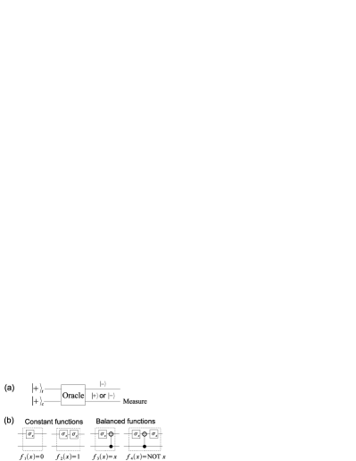
Figure 1: (a) Schematic illustration of the Deutsch-Josza algorithm. (b) The quantum networks for all possible oracles. The inter-line symbol in the network denotes the controlled-NOT gate $|0\rangle\langle 0|^{(c)}\otimes\mathbb{I}^{(t)}+|1\rangle\langle 1|^{(c)}\otimes\sigma_{x}^{(t)}$, where the superscripts denote the qubits and $\mathbb{I}$ is identity.

To implement the DJ algorithm one should be able to construct all the possible four configurations (Fig. 1(b)). We find it is sufficient to do these on the star-like 4-qubit graph state with appropriate single-qubit measurement sequences and corresponding feed-forwards. We start with the introduction of the general logical quantum circuit that can be realized on the star-like 4-qubit graph (Fig. 2(a)), with arbitrary logical input states and arbitrary single-qubit measurement bases in the $x$-$y$ plane. For this purpose, as in Ref. onewayPRL , we first prepare the four physical qubits in the graph into the initial state $|\psi_{t}\rangle_{1}\otimes|+\rangle_{2}\otimes|+\rangle_{3}\otimes|\psi_{c}\rangle_{4}$, where the two arbitrary logical input states $|\psi_{t}\rangle$ and $|\psi_{c}\rangle$ of the two logical qubits eworkn1 (a target qubit and a control qubit) are initially encoded on the physical qubits 1 and 4. Then all physical qubits are entangled by the entangling operator

$$S=S^{(12)}S^{(23)}S^{(42)},$$ (1)

where $S^{(jk)}=|0\rangle\langle 0|^{(j)}\otimes\sigma_{z}^{(k)}+|1\rangle\langle 1|^{(j)}\otimes\mathbb{I}^{(k)}$ is a controlled-phase gate applied on the physical qubits $j$ and $k$ cphase . The logical information is now delocalized. It is then manipulated by the measurements carried on the physical qubits 1 and 2 with the bases $B_{1}(\alpha_{1})=\{|\alpha_{1+}\rangle_{1},|\alpha_{1-}\rangle_{1}\}$ and $B_{2}(\alpha_{2})=\{|\alpha_{2+}\rangle_{2},|\alpha_{2-}\rangle_{2}\}$ respectively, where $|\alpha_{\pm}\rangle=\frac{1}{\sqrt{2}}(|0\rangle\pm e^{i\alpha}|1\rangle)$ and $\alpha_{1},\alpha_{2}$ are arbitrary angles. After the measurements the logical target qubit is transferred to the physical qubit 3, while the logical control qubit is still encoded on the physical qubit 4. The effective logical quantum circuit performed on the two logical qubits for the above process is shown in Fig. 2(b). The $s_{1}$ and $s_{2}$ in the circuit denote the outcome of the two measurements, where $s_{j}=0(1)$ corresponds to the output state $|\alpha_{j+}\rangle(|\alpha_{j-}\rangle)$ ($j=1,2$). The presence of the $s_{1}$ and $s_{2}$ represents the randomness introduced by the single-qubit projective measurements. In one-way QC appropriate feed-forwards onewayPRL compensate for this randomness to restore the determinacy of the computing.

Figure 2: (a) The star-like 4-qubit graph. The vertices represent the four physical qubits, and each edge between them indicates a controlled-phase gate applied on the connected qubits when to produce the entangled state. The arrows marked on vertices 1 and 2 denote the measurements. For the detailed description of the initial state, entangling, and measurements, see the text. (b) The general logical quantum circuit realized on the above graph with arbitrary logical input states and arbitrary measurement bases. $R_{n}(\alpha)=e^{-i\alpha\sigma_{n}/2}$ $(n=x,z)$

The design of the resource entangled state and the single-qubit measurement sequences for implementing the DJ algorithm is done by comparing the general logical circuit in Fig. 2(b) with the networks in Fig. 1(b). Since the input state in the DJ algorithm is $|+\rangle\otimes|+\rangle$, we set $|\psi_{t}\rangle=|\psi_{c}\rangle=|+\rangle$. The resulted entangled state, $|\psi_{\text{G}}\rangle=(|+\rangle_{1}|0\rangle_{2}|-\rangle_{3}|+\rangle_{4}+|-\rangle_{1}|1\rangle_{2}|+\rangle_{3}|-\rangle_{4})/\sqrt{2}$, which is produced by performing the entangling operator $S$ on the initial state $|+\rangle_{1}\otimes|+\rangle_{2}\otimes|+\rangle_{3}\otimes|+\rangle_{4}$, is exactly the 4-qubit graph state which corresponds to the star-like 4-qubit graph onewayPRA (it is also equivalent to the 4-qubit GHZ state under local unitary operations). The measurement bases and the corresponding feed-forward operations which are chosen to reproduce the networks of all possible oracles are summarized in the Table 1. Note in the design of the measurements which correspond to the constant functions $f_{1}$ and $f_{2}$, the fact is used that a CNOT gate is equivalent to the identity operation when it acts on the state $|+\rangle\otimes|+\rangle$. The final result of the algorithm is read by measuring the physical qubit 4. If its state (after accounting for the feed-forward operation) is $|+\rangle(|-\rangle)$ then the function is constant(blanced).

Table 1: Measurement bases and feed-forward operations for implementing the DJ algorithm. $\text{FF}^{(3)}$ and $\text{FF}^{(4)}$ represent the feed-forward operations on physical qubits 3 and 4.

	Measurement bases	$\text{FF}^{(3)}$	$\text{FF}^{(4)}$
$f_{1}$	$B_{1}(0),B_{2}(0)$	$\sigma_{z}^{s_{1}}\sigma_{x}^{s_{2}+1}$	$\sigma_{z}^{s_{1}}$
$f_{2}$	$B_{1}(0),B_{2}(0)$	$\sigma_{z}^{s_{1}}\sigma_{x}^{s_{2}}$	$\sigma_{z}^{s_{1}}$
$f_{3}$	$B_{1}(\pi),B_{2}(0)$	$\sigma_{z}^{s_{1}+1}\sigma_{x}^{s_{2}}$	$\sigma_{z}^{s_{1}}$
$f_{4}$	$B_{1}(\pi),B_{2}(0)$	$\sigma_{z}^{s_{1}+1}\sigma_{x}^{s_{2}+1}$	$\sigma_{z}^{s_{1}}$

III Experiment

III.1 Graph state generation

We used the spins of the four ¹³C nuclei in the crotonic acid dissolved in $\text{D}_{2}\text{O}$ (see Fig. 3) as the four physical qubits, which provide the reduced hamiltonian $H_{0}=\sum_{j=1}^{4}\omega_{j}I_{z}^{(j)}+2\pi\sum_{j<k}^{4}J_{jk}I_{z}^{(j)}I_{z}^{(k)}$ with the Larmor angular frequencies $\omega_{j}$ and $J$-coupling strengths $J_{jk}$. On a Bruker UltraShield 500 spectrometer at room temperature, the measured parameters are listed in Fig. 3 and their relaxation times are obtained as $T_{1}(C1)=12.37s$, $T_{1}(C2)=4.89s$, $T_{1}(C3)=4.13s$, $T_{1}(C4)=4.96s$, $T_{2}(C1)=376.2ms$, $T_{2}(C2)=506.7ms$, $T_{2}(C3)=566.5ms$, $T_{2}(C4)=544.5ms$. In experiments, we labelled the nuclei spins C2, C4, C3, C1 as the physic qubits 1, 2, 3, 4 in Fig. 2.

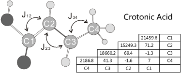
Figure 3: Molecular structure of crotonic acid with a table of the chemical shifts (on the diagonal) and $J$-coupling constants (below the diagonal). The parameters are given in unit Hz.

Figure 4: Network for implementing the one-way DJ algorithm, consisting of the main three stages: (i) graph state generation, (ii) single-qubit measurements and (iii) feed-forward correction. Here $\text{H}=e^{-i\frac{\pi}{4}\sigma_{y}}$ is the pseudo-Hadamard gate with its conjugate ${H^{+}}$, and $\text{G}_{z}$ is the pulsed magnetic filed gradient along z axis. In the feed-forward process, the controlled gates are performed by the conditionality on the controlling spin being in the $|0\rangle$ or $|1\rangle$ state, which are determined by the values of (A, B): (A, B) = (0, 1), (1, 1), (1, 0) and (0, 0) correspond to the functions $f_{1}$ to $f_{4}$.

We first initialized the NMR ensemble to a standard pseudopure state with deviation $|0000\rangle\langle 0000|$ from the thermal equilibrium state using the spatial average technique spatial . Then a 4-qubit GHZ state $|\psi\rangle_{GHZ}=(|0110\rangle+|1001\rangle)/\sqrt{2}$ can be created from $|0000\rangle$ by the network shown in Fig. 4. Here, the controlled-not gate $\text{CNOT}^{(jk)}$ could be further decomposed into

$$R_{-z}^{(k)}(\frac{\pi}{2})-R_{-z}^{(j)}(\frac{\pi}{2})-R_{-x}^{(k)}(\frac{\pi}{2})-e^{-i\frac{\pi}{4}\sigma_{z}^{(j)}\sigma_{z}^{(k)}}-R_{y}^{(k)}(\frac{\pi}{2}),$$ (2)

where $R_{y}^{(k)}(\frac{\pi}{2})=e^{-i(\pi/4)\sigma_{y}^{(k)}}$ denotes a $\frac{\pi}{2}$-rotation of the qubit $k$ around the $\hat{y}$ axis, and so forth. The $J$-coupling gate $e^{-i\frac{\pi}{4}\sigma_{z}^{(j)}\sigma_{z}^{(k)}}$ can be realized by the free evolution of the spin system under $H_{0}$ with appropriate refocusing pulses. Those $\hat{z}$ rotations in CNOT gates can be omitted due to the initial state $|0000\rangle$nmrreview . Such a GHZ state has the total zero spin quantum number that facilitates us to clean-up the state further by a pulsed magnetic field gradient ernst . Finally, the graph state $|\psi_{\text{G}}\rangle$ is generated from the GHZ state by the local operations $R_{-y}^{(1)}(\frac{\pi}{2})R_{-y}^{(3)}(\frac{\pi}{2})R_{-y}^{(4)}(\frac{\pi}{2})$.

In experiments, all the single-qubit operations are realized by sequences of strongly modulating NMR pulses created by GRAPE algorithm grape . We maximized the gate fidelity of the simulated propagator to the ideal gate, taking into account of radio frequency (RF) inhomogeneity. Theoretically the gate fidelities we calculated for every pulse are greater than 0.99, and all the pulse lengths are 600 $\mu s$.

In order to access the quality of the graph state we prepared, we employed the state tomography process tomo to obtain the reconstructed density matrix $\rho_{\text{exp}}$. Since only single-quantum coherences can be directly observed, the tomography involves 19 repetitions of the experiment, each with a different readout pulse sequence aaa by taking consideration of some unresolved J couplings. The real part of the reconstructed density matrix is shown in Fig. 5 along with the theoretical expectation. The imaginary part is small comparable to zero in the theoretical expectation. To quantify how close the prepared state $\rho_{\text{exp}}$ to the theoretical one $\rho_{id}$, we used the measure of the attenuated correlation defined by $c(\rho_{exp})=Tr(\rho_{id}\rho_{exp})/\sqrt{Tr(\rho_{id}^{2})}$, which takes into account both systematic errors and the net loss of magnetization due to random errors and decoherence. The value of the correlation for the tomographic readout of the GHZ state $|\psi\rangle_{GHZ}$ is $c(\rho_{GHZ}^{exp})=0.73$, compared to the simulated value 0.80 where we adopted the decoherence model corr to take the loss of magnetization due to spin relaxation. The experimental time for the preparation is around 85 $ms$. To remove the effect of the net loss of magnetization due to random errors and spin relaxation, we also calculated the fidelity defined corr2 by $F_{GHZ}=Tr(\rho_{id}\rho_{exp})/\sqrt{Tr(\rho_{id}^{2})Tr(\rho_{exp}^{2}))}$, which yields the value of 0.88. Due to the imperfection of GRAPE pulses calculated and the effect of strongly-coupling, the total theoretical fidelity is around 0.92. Moreover, the lower experimental fidelity of 0.88 is mainly caused by other uncertainties (e.g., the imperfection of the static magnetic field) in the experiments. The correlation of the graph state $|\psi_{G}\rangle$ is similar to the state $|\psi_{GHZ}\rangle$, because it was created only by local operations.

Moreover, we confirmed the generation of the four-partite pseudo-entanglement by obtaining a negative expectation value of the entanglement witness witness $W=I/2-|\psi_{\text{GHZ}}\rangle\langle\psi_{\text{GHZ}}|$ ($I$ denotes identity operator) from the tomographic readout: Tr$(W\rho_{\text{exp}})=-0.175$.

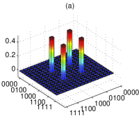
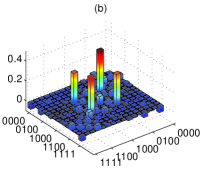
Figure 5: (color online) The ideal (a) and measured (b) density matrices of the four-qubit GHZ state $|\psi\rangle_{GHZ}=(|0101\rangle+|1010\rangle)/\sqrt{2}$. The rows and columns are numbered with the computational basis states.

III.2 Implementation of DJ algorithm

The required single-qubit projective measurements in the one-way QC are absent in current NMR quantum computing technologies. But instead we can use the pulsed magnetic field gradients to mimic them measure , whose effects are equivalent to that by applying these projective measurements on every member of the ensemble. For example, one could use the operations

$$P_{z}^{(1)}:G_{1}-R_{y}^{(2)}(\pi)-R_{y}^{(4)}(\pi)-G_{1}-R_{y}^{(3)}(\pi)-R_{y}^{(4)}(\pi)$$

$$-G_{1}-R_{-y}^{(2)}(\pi)-R_{-y}^{(4)}(\pi)-G_{1}-R_{-y}^{(3)}(\pi)-R_{-y}^{(4)}(\pi)$$ (3)

to mimic the $\sigma_{z}^{(1)}$ measurement on the physical qubit 1, where $G_{1}$ is the pulsed magnetic field gradient along $\hat{z}$ with a period of $\tau_{1}/4$. These operations dephase all the coherences which are associated with the transitions of qubit 1 in the density matrix $\rho=|\Phi\rangle\langle\Phi|$ (suppose $|\Phi\rangle=|0\rangle_{1}|\phi_{0}\rangle+|1\rangle_{1}|\phi_{1}\rangle$, where $|\phi_{0(1)}\rangle$ is the state of the other three qubits), resulting in an ensemble-average density matrix $|0\rangle_{1}\langle 0||\phi_{0}\rangle\langle\phi_{0}|+|1\rangle_{1}\langle 1||\phi_{1}\rangle\langle\phi_{1}|$, which is exactly the same as the outcome by performing projective measurement $\sigma_{z}^{(1)}$ on every member of the ensemble. To mimic the measurement $\sigma_{x}^{(1)}$, one just first rotate the qubit 1 to the $\hat{z}$ axis before $P_{z}^{(1)}$. In our experiment we use the sequences $R_{-y}^{(1)}(\frac{\pi}{2})-P_{z}^{(1)}$ and $R_{y}^{(1)}(\frac{\pi}{2})-P_{z}^{(1)}$ to mimic the measurements with the bases $B_{1}(0)$ and $B_{1}(\pi)$ respectively. Therefore the different outcomes are labeled in the different subspaces of qubit 1 denoted by $|0\rangle_{1}\langle 0|$(i.e., $s_{1}=0$) and $|1\rangle_{1}\langle 1|$ (i.e., $s_{1}=1$). The measurement on qubit 2 with basis $B_{1}(0)$ is mimicked by a similar sequence $R_{-y}^{(2)}(\frac{\pi}{2})-P_{z}^{(2)}$, where

$$P_{z}^{(2)}:R_{y}^{(3)}(\pi)-R_{y}^{(4)}(\pi)-G_{2}-R_{y}^{(1)}(\pi)-R_{y}^{(4)}(\pi)-G_{2}$$

$$-R_{-y}^{(3)}(\pi)-R_{-y}^{(4)}(\pi)-G_{2}-R_{-y}^{(1)}(\pi)-R_{-y}^{(4)}(\pi)-G_{2},$$ (4)

where $G_{2}$ is the pulsed magnetic field gradient with a period of $\tau_{2}/4$.

After the measurements, the computational outcomes have been stored in the different subspaces depending on the measurement results $s_{1}$ and $s_{2}$. However, to obtain a deterministic and correct computation, the feed-forward operations should be carried out conditionally on the measurement results $s_{1}$ and $s_{2}$. We also experimentally realized the feed-forward operations by the conditional unitary operations illustrated in Fig. 4. After this, the judgement of whether the function $f$ is constant or balanced is determined by measuring the state of qubit 4: if the state of qubits is in $|+\rangle$, the function $f$ is constant; conversely, if the state of qubits is in $|-\rangle$, the function $f$ is balanced. As a result of $|\pm\rangle\langle\pm|=\frac{1}{2}I\pm\sigma_{x}$, the $|+\rangle/|-\rangle$ state will give a positive/negative NMR signal if we first reference the spectrum of the thermal equilibrium after a $[\frac{\pi}{2}]_{y}$ pulse as a positive one. The results are shown in Fig. 6 for four cases $f_{1}-f_{4}$. In (a) and (b), the signal amplitude is positive, which indicates the state of qubit 4 is in $|+\rangle$ and the function $f$ is constant. In (c) and (d), the signal is inverted which indicates the state of qubit 4 is in $|-\rangle$ and the function $f$ is balanced. Here the carbon signal-to-noise ratio (Signal/Noise) of the spectra is about 44.4-48.3. The imperfection of the experimental spectra compared to the simulated spectra is mainly caused by the unideal input graph state, the imperfection of the static magnetic field and the GRAPE pulses. Alternatively, the feed-forward process can also be replaced by the single-qubit measurement under a suitable basis onewayPRL , which makes that the one-way QC can be completed solely by single-qubit measurements.

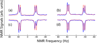
Figure 6: (color online) The experimental (line) and simulated (dotted line) spectra of qubit 4 for one-way DJ algorithm: (a)-(b) for the constant functions $f_{1}$ and $f_{2}$, (c)-(d) for the balanced functions $f_{3}$ and $f_{4}$.

IV Conclusion

We realized the complete process of deterministic one-way QC using a star-like 4-qubit graph state in NMR: the graph state was generated deterministically by exploiting the existing particle-particle interactions in our experiments; the single qubit measurements were mimicked by pulsed magnetic field gradients; and the feed-forward corrections were realized by conditional-unitary gates in our specific NMR system. Here NMR technique is used as a test-bed for the demonstration of deterministic one-way QC, however, it does not imply that any of the results obtained are specific to NMR. The experience obtained from our experiments could be helpful to other physical systems for future scalable deterministic one-way QC and deserve further investigation. If the direct particle-particle interactions of the quantum system (such as trapped ions and optical lattices) are provided, one can prepare the cluster state deterministically, do single-qubit measurements, and perform the feed-forward correction by unitary gates, therefore realizing scalable one-way QC deterministically.

- (1) R. Raussendorf and H. J. Briegel, Phys. Rev. Lett. 86, 5188 (2001).
- (2) R. Raussendorf, D. E. Browne, and H. J. Briegel, Phys. Rev. A 68, 022312 (2003).
- (3) M. A. Nielsen and I. L. Chuang, Quantum Computation and Quantum Information (Cambridge University Press, Cambridge, England, 2000).
- (4) H. J. Briegel and R. Raussendorf, Phys. Rev. Lett. 86, 910 (2001).
- (5) M. Van den Nest, A. Miyake, W. Dür, and H. J. Briegel, Phys. Rev. Lett. 97, 150504 (2006).
- (6) P. Walther et al., Nature 434, 169 (2005).
- (7) P. Walther, M. Aspelmeyer, K. J. Resch, and A. Zeilinger, Phys. Rev. Lett. 95, 020403 (2005); N. Kiesel et al., Phys. Rev. Lett. 95, 210502 (2005); A.-N. Zhang et al., Phys. Rev. A 73, 022330 (2006); C.-Y. Lu et al., Nature Phys. 3, 91 (2007); G. Vallone et al., Phys. Rev. Lett. 98, 180502 (2007).
- (8) X. Su et al., Phys. Rev. Lett. 98, 070502 (2007).
- (9) R. Prevedel et al., Nature 445, 65 (2007).
- (10) K. Chen et al., Phys. Rev. Lett. 99, 120503 (2007).
- (11) G. Vallone, E. Pomarico, F. De Martini, and P. Mataloni, Phys. Rev. Lett. 100, 160502 (2008).
- (12) M. S. Tame et al., Phys. Rev. Lett. 98, 140501 (2007).
- (13) D. Deutsch and R. Jozsa, Proc. R. Soc. London A 439, 553 (1992).
- (14) Note that some papers use another controlled-phase gate as the entangling operator. The produced graph states with these two entangling operators are equivalent up to local unitary operations.
- (15) D. G. Cory, M. D. Price, and T. F. Havel, Physica D 120, 82 (1998).
- (16) L. M. K. Vandersypen and I. L. Chuang, Rev. Mod. Phys. 76, 1037 (2005).
- (17) R. R. Ernst, G. Bodenhausen, A. Wokaun, Principles of Nuclear Magnetic Resonance in One and Two Dimensions, Clarendon Press, Oxford, 1987.
- (18) N. Khanejaa, T. Reiss et al., Journal of Magnetic Resonance 172, 296-305 (2005).
- (19) J. S. Lee, Phys. Lett. A 305, 349 (2002).
- (20) The 19 readout pulse sequences: X1Y2, Y2X3, X2X3, Y1X2X4, Y1X3Y4, Y1, Y3, YY1X2Y3, Y1X2Y3YX1Y2Y3X4, X2Y3YX1Y2, X2Y3YX1Y2X3, X2X3YY1Y2, X1X2Y3Y4, Y1Y2X3X4, X2XX1X2X3X4, YX1X2X3Y4, X2Y, Y3YY1Y2Y3X4, Y1X3XY2X3X4, where Xi(Yi) denotes a pulse around the X(Y) axis for the qubit , and denotes the J-coupling evolution between qubit and for a period of .
- (21) Lieven M. K. Vandersypen, Matthias Steffen et al., Nature 414, 883-887
- (22) N. Boulant, E.M. Fortunato, M.A. Pravia, G. Teklemariam, D.G. Cory, and T.F. Havel, Phys. Rev. A 65, 024302 (2002).
- (23) G. Tóth and O. Gühne, Phys. Rev. A 72, 022340 (2005).
- (24) G. Teklemariam, E. M. Fortunato, M. A. Pravia, T. F. Havel, and D. G. Cory, Phys. Rev. Lett. 86, 5845 (2001).