Substructure and Scatter in the Mass–Temperature Relations of Simulated Clusters

Abstract

Galaxy clusters exhibit regular scaling relations among their bulk properties. These relations establish vital links between halo mass and cluster observables. Precision cosmology studies that depend on these links benefit from a better understanding of scatter in the mass-observable scaling relations. Here we study the role of merger processes in introducing scatter into the $M$-$T_{\rm X}$ relation, using a sample of 121 galaxy clusters simulated with radiative cooling and supernova feedback, along with three statistics previously proposed to measure X-ray surface brightness substructure. These are the centroid variation ($w$), the axial ratio ($\eta$), and the power ratios ($P_{20}$ and $P_{30}$). We find that in this set of simulated clusters, each substructure measure is correlated with a cluster’s departures $\delta\ln T_{\rm X}$ and $\delta\ln M$ from the mean $M$-$T_{\rm X}$ relation, both for emission-weighted temperatures $T_{\rm EW}$ and for spectroscopic-like temperatures $T_{\rm SL}$, in the sense that clusters with more substructure tend to be cooler at a given halo mass. In all cases, a three-parameter fit to the $M$-$T_{\rm X}$ relation that includes substructure information has less scatter than a two-parameter fit to the basic $M$-$T_{\rm X}$ relation.

1. Introduction

Clusters of galaxies play a critical role in our understanding of the Universe and its history and are potentially powerful tools for conducting precision cosmology. For example, large cluster surveys can discriminate between cosmological models with different dark-energy equations of state by providing complementary observations of the shape of the cluster mass function, evolution in the number density of clusters with redshift, and bias in the spatial distribution of clusters (Wang & Steinhardt, 1998; Levine et al., 2002; Hu, 2003; Majumdar & Mohr, 2004; Voit, 2005). However, this potential to put tight constraints on the properties of dark energy will be realized only if we can accurately measure the masses of clusters and can precisely characterize the scatter in our mass measurements.

Scatter in X-ray cluster properties is directly related to substructure in the intracluster medium. If clusters were all structurally similar, then there would be a one-to-one relationship between halo mass and any given observable property. Generally speaking, deviations from a mean mass-observable relationship are attributed to structural differences among clusters. One kind of structural difference is the presence or absence of a cool core, in which the central cooling time is less than the Hubble time at the cluster’s redshift, and the prominence of a cool core is observed to be a source of scatter in scaling relationships (Fabian et al., 1994; Markevitch, 1998; Voit et al., 2002; McCarthy et al., 2004). We also expect structural differences to arise from substructure in the dark matter, galaxy, and gas distributions. For instance, there may be a spread in halo concentration at a given mass, variations in the incidence of gas clumps, differences in the level of AGN feedback, or various effects due to mergers. All of these deviations can be considered forms of substructure that produce scatter in the mass-observable relations one would like to use for cosmological purposes. While it may ultimately be possible to constrain the amount of scatter and its evolution with redshift using self-calibration techniques (Lima & Hu, 2005), such constraints would be improved by prior knowledge about the relationship between scatter and substructure.

Traditionally, the most worrisome form of substructure has been that due to the effects of merger events. Clusters are often identified as “relaxed” or “unrelaxed”, with the former assumed to be nearly in hydrostatic equilibrium and the latter suspected of being far from equilibrium. Cosmological simulations of clusters indicate that the truth is somewhere in between. The cluster population as a whole appears to follow well-defined virial relations with log-normal scatter around the mean, showing that clusters do not cleanly separate into relaxed and unrelaxed systems (e.g.,Evrard et al. (2007)). Even the most relaxed-looking clusters are not quite in hydrostatic equilibrium (e.g.,Kravtsov et al. (2006)). Instead of simply being “relaxed” or “unrelaxed,” clusters occupy a continuum of relaxation levels determined by their recent mass-accretion history.

Quantifying this continuum of relaxation offers opportunities for reducing scatter in the mass-observable relations. If mergers are indeed responsible for much of the observed scatter around a given scaling relation, then there may be correlations between a cluster’s morphology and its degree of deviation from the mean relation. Once one identifies a morphological parameter that correlates with the degree of deviation, one can construct a new mass-observable relation with less scatter by including the morphological parameter in the relation. Such an approach would be analogous to the improvement of Type Ia supernovae as distance indicators by using light-curve stretch as a second parameter to indicate the supernova’s luminosity (Phillips, 1993; Riess et al., 1996).

Here we investigate how merger-related substructure in simulated clusters affects the relationship between a simulated cluster’s mass and the temperature of its intracluster medium, building upon Buote & Tsai (1995) and O’Hara et al. (2006). Buote & Tsai (1995) quantified the morphologies and dynamical states of observed clusters and found structure measures to be an indicator of the dynamical state of a cluster. O’Hara et al. (2006) also examined morphological measurements, for both observed and simulated clusters, and found that simulations without cooling showed no correlation between substructure and scaling relation scatter. In this work we examine substructure for simulated clusters with radiative cooling and focus on the idea that merger processes introduce intrinsic scatter into the $M$-$T_{\rm X}$ relationship by displacing clusters in the $M$-$T_{\rm X}$ plane away from the mean X-ray temperature $\langle{T_{\rm X}}\rangle|_{{}_{M}}$ at a given mass $M$, either to higher or lower average ICM temperature. We then adopt a set of statistics (Buote & Tsai, 1995; O’Hara et al., 2006) for quantifying galaxy cluster substructure and merger activity in order to investigate this hypothesis. Section 2 discusses the $M$-$T_{\rm X}$ scaling relationship in our sample of simulated clusters and shows that disrupted-looking clusters in this sample tend to be cooler at a given cluster mass. In Section 3 we attempt to quantify the relationship between morphology and temperature using four different substructure statistics and compare it to similar studies. We then show that substructure in these simulated clusters indeed correlates with scatter in the $M$-$T_{\rm X}$ relationship and assess the prospects for using that correlation to reduce scatter in the $M$-$T_{\rm X}$ plane. Section 4 summarizes our results.

2. Mass-Temperature Relation in Simulated Clusters

This study is based on an analysis of 121 clusters simulated using the cosmological hydrodynamics TREE+SPH code GADGET-2 (Springel, 2005), which were simulated in a standard $\Lambda$ cold dark matter ($\Lambda$CDM) universe with matter density $\Omega_{M}$ = 0.3, $h$ = 0.7, $\Omega_{b}$ = 0.04, and $\sigma_{8}$ = 0.8. The simulation treats radiative cooling with an optically-thin gas of primordial composition, includes a time-dependent UV background from a population of quasars, and handles star formation and supernova feedback using a two-phase fluid model with cold star-forming clouds embedded in a hot medium. All but four of the clusters are from the simulation described in Borgani et al. (2004), who simulated a box $192\,h^{-1}\,{\rm Mpc}$ on a side, with $480^{3}$ dark matter particles and an equal number of gas particles. The present analysis considers the 117 most massive clusters within this box at $z=0$, which all have $M_{200}$ greater than $5\times 10^{13}\,h^{-1}M_{\odot}$. By convention, $M_{\Delta}$ refers to the mass contained in a sphere which has a mean density of $\Delta$ times the critical density $\rho_{c}$, and whose radius is denoted by $R_{\Delta}$

That cluster set covers the $\sim$1.5-5 keV temperature range, but the $192\,h^{-1}\,{\rm Mpc}$ box is too small to contain significantly hotter clusters. We therefore supplemented it with four clusters with masses $>10^{15}\,h^{-1}\,M_{\odot}$ and temperatures $>5$ keV drawn from a dark-matter-only simulation in a larger $479\,h^{-1}\,{\rm Mpc}$ box (Saro et al., 2006). The cosmology for this simulation also was $\Lambda$CDM, but with $\sigma_{8}$ = 0.9. These were then re-simulated including hydrodynamics, radiative cooling, and star formation, again with GADGET-2 and using the zoomed-initial-conditions technique of Tormen (1997), with a fourfold increase in resolution. This is comparable to the resolution of the clusters in the smaller box. Adding these four massive clusters to our sample gives a total of 121 clusters with $M_{200}$ in the interval $5\times 10^{13}\,h^{-1}M_{\odot}$ to $2\times 10^{15}\,h^{-1}M_{\odot}$.

We first need to specify our definitions for mass and temperature. In this paper, cluster mass refers to $M_{200}$. For temperature, we use two definitions. The first is the emission-weighted temperature

$$T_{\rm EW}=\frac{\int T[n^{2}\Lambda(T)]\,d^{3}x}{\int n^{2}\Lambda(T)\,d^{3}x}\;\;,$$ (1)

where $n$ is the electron number density and $\Lambda(T)$ is the usual cooling function for intracluster plasma. The second is the spectroscopic-like temperature of Mazzotta et al. (2004),

$$T_{\rm SL}=\frac{\int T[n^{2}T^{-3/4}]\,d^{3}x}{\int n^{2}T^{-3/4}\,d^{3}x}\;\;,$$ (2)

where the power-law weighting function replacing $\Lambda(T)$ is chosen so that $T_{\rm SL}$ approximates as closely as possible the temperature that would be determined from fitting a single-temperature plasma emission model to the integrated spectrum of the intracluster medium. The presence of metals in the ICM of real clusters introduces line emission that complicates the computation of $T_{\rm SL}$ for clusters $<$3 keV (Vikhlinin, 2006). However, the simulated spectra for the clusters in our sample are modelled with zero metallicity, which eases this restriction in our analysis.

Figure 1 shows the mass-temperature relations based on these definitions for our sample of simulated clusters. The best fits to the power-law form

$$M=M_{0}\left(\frac{T_{\rm X}}{3\,{\rm keV}}\right)^{\alpha}$$ (3)

have the coefficients $M_{0}\simeq 5.9\times 10^{13}\ h^{-1}M_{\odot},\alpha\simeq 1.5$ for $T_{\rm X}$ corresponding to $T_{\rm SL}$ and $M_{0}\simeq 4.4\times 10^{13}\ h^{-1}M_{\odot},\alpha\simeq 1.4$ for $T_{\rm X}$ corresponding to $T_{\rm EW}$. As is generally the case for simulated clusters, the power-law indices of the mass-temperature relations found here are consistent with cluster self-similarity and the virial theorem (Kaiser, 1986; Navarro et al., 1995). These relationships have scatter, which we characterize by the standard deviation in log space $\sigma_{\ln M}$ about the best-fit mass at fixed temperature $T_{\rm X}$. When relating $M$ to the emission-weighted temperature $T_{\rm EW}$, we find $\sigma_{\ln M}=0.102$. When relating cluster mass $M$ to the spectroscopic-like temperature $T_{\rm SL}$, the scatter is $\sigma_{\ln M}=0.127$. That the scatter is larger for the spectroscopic-like temperature is not surprising, given the sensitivity of $T_{\rm SL}$ to the thermal complexity of the ICM.

Figure 1.— Mass-temperature ($M$-$T_{\rm X}$) relationships for the 121 clusters in our sample. Spectroscopic-like temperature $T_{\rm SL}$ is plotted in the top panel, while emission-weighted temperature $T_{\rm EW}$ is plotted in the bottom panel. The solid lines show the best-fit power-law relation $M=M_{0}(T_{\rm X}/3\ {\rm keV})^{\alpha}$ over the whole sample, while the dashed lines show the best-fit relation for systems with $T_{\rm X}>$ 2 keV. Open circles represent the clusters that have the greatest positive temperature offset from the mean relationship, and filled circles represent the clusters with the greatest negative temperature offset.

Figure 1 also highlights two subsamples for each definition of temperature, selected based on the clusters’ deviations in $\ln T_{\rm X}$ space from the mean mass-temperature relation. In each panel, open circles represent the eight clusters that have the largest positive deviations and are therefore “hotter” than other clusters of the same mass, while filled circles represent the eight with the largest negative deviation and are “cooler” than other clusters of the same mass. In general, these temperature estimates are well correlated, so that hotter outliers in $T_{\rm EW}$ are also hotter outliers in $T_{\rm SL}$ and cooler outliers in $T_{\rm EW}$ are also cooler outliers in $T_{\rm SL}$. Since Figure 1 distinguishes the most extreme outliers for the two temperature estimates, this distinction may define slightly different sets, though they still overlap.

Figure 2 presents a gallery of surface brightness maps for two sets of eight clusters with the most extreme offsets from the mean $M$-$T_{\rm SL}$ relation. The eight unusually hot clusters are in the top panel, and the eight cooler clusters are in the bottom panel. In these plots the hotter clusters appear more symmetric, and are seemingly “more relaxed,” and the cooler clusters appear less symmetric and seemingly “less relaxed.” The gallery as a whole therefore suggests that relaxed clusters tend to be hot for their mass and unrelaxed clusters tend to be cool for their mass.

Figure 2.— Surface-brightness contour maps for sixteen of the clusters in our sample, overlaid with a circular aperture of radius $R_{500}$. The top panel has eight maps representing the clusters that have the largest positive deviation $\delta\ln T_{\rm X}$ from the mean $M$-$T_{\rm X}$ relation, calculated using the spectroscopic-like temperature $T_{\rm SL}$. These are the objects represented by open circles in the top panel of Figure 1. The bottom panel has eight maps representing the clusters that have the largest negative deviation from the same $M$-$T_{\rm X}$ relationship, represented by the filled circles in Figure 1. Note that the “hotter” clusters in the top panel appear more symmetric, while the “cooler” clusters in the bottom panel appear more irregular.

At first glance, the result that disrupted-looking clusters in cosmological simulations tend to be cooler than other clusters of the same mass may seem counterintuitive, since one might expect that mergers ought to produce shocks that raise the mean temperature of the intracluster medium. This finding has also been noted by Mathiesen & Evrard (2001) and Kravtsov et al. (2006). Cluster systems in the process of merging tend to be cool for their total halo mass because much of the kinetic energy of the merger has not yet been thermalized.

The idealized simulations of Poole et al. (2007) illustrate what may happen to the ICM temperature during a single merger. Before the cores of the two merging systems collide, the mean temperature is cool for the overall halo mass because it is still approximately equal to the pre-merger temperature of the two individual merging halos. There is a brief upward spike in temperature when the cores of the merging halos collide, after which the system is again cool for its mass. Then, as the remaining kinetic energy of the merger thermalizes over a period of a few billion years, the temperature gradually rises to its equilibrium value. The merging system therefore spends a considerably longer time at relatively cool values of mean temperature for its halo mass than at relatively hot values. Hence, such simulations suggest a possible explanation for why more relaxed systems would tend to lie on the hot side of the $M$-$T_{\rm X}$ relation, while disrupted systems would tend to lie on the cool side. A caveat, however, is that the current generation of hydrodynamic cluster simulations tend to produce relaxed clusters whose temperature profiles continue to rise to smaller radii than is observed in real clusters (Tornatore et al., 2003; Nagai et al., 2007), potentially enhancing average temperatures for such systems. As a separate test of this effect, we excise the core regions from our sample clusters, calculate new substructure measures and new emission-weighted temperatures for the core-excised clusters, and repeat our analysis.

3. Quantifying Substructure

The question we would like to address in this study is whether the surface-brightness substructure evident in Figure 2 is well enough correlated with deviations from the mean mass-temperature relation to yield useful corrections to that relation. In order to answer that question, we need to quantify the surface-brightness substructure in each cluster image, so that we can determine the degree of correlation across the entire sample. O’Hara et al. (2006) explored the relationship between cluster structure and X-ray scaling relations in both observed and simulated clusters, and we adopt their suite of substructure measures in this study. These include centroid variation, axial ratio, and the power ratios of Buote & Tsai (1995). In this section we define and discuss those statistics and apply them to surface-brightness maps made from three orthogonal projections of each cluster. Then we assess how well these statistics correlate with offsets from the mean mass-temperature relation.

3.1. Axial Ratio

The axial ratio $\eta$ for a cluster surface-brightness map is a measure of its elongation, which is of interest because it has been found from simulations that the ICM is often highly elongated during merger events (Evrard et al., 1993; Pearce et al., 1994). It is computed from the second moments of the surface brightness,

$$M_{ij}=\sum I_{\rm X}x_{i}x_{j}.$$ (4)

The summation is conducted over the coordinates $(x_{1},x_{2})$ of the pixels that lie within an aperture centered at the origin of the coordinate system to which $(x_{1},x_{2})$ refer. Following the work of O’Hara et al. (2006), we use an aperture of radius $R_{500}$ centered on the brightness peak. We then compute $\eta$ from the ratio of the non-zero elements that result from diagonalizing the matrix $M$. That is,

$$D=U^{T}MU,$$ (5)

where $U$ is a diagonalizing matrix for $M$, and

$$\eta=\left\{\begin{array}[]{ll}\frac{D_{12}}{D_{21}},&D_{12}\leq D_{21}\\ \frac{D_{21}}{D_{12}},&D_{12}>D_{21}\end{array}\right\}\;\;.$$ (6)

The axial ratio is therefore defined to be in the range $\eta\in[0,1]$, with $\eta=1$ for a circular cluster. Of course there are other choices for the origin of the coordinate system, besides using the brightness peak. For instance, in order to avoid misplaced apertures yielding artificially low axial ratios for nearly circular distributions, one could adjust the position of the aperture to seek a maximum in $\eta$. Doing this, we sometimes find that $\eta\approx 1$ even for non-circular clusters, as is evident in Figure 3. This figure depicts the surface-brightness map of what appears to be a disturbed cluster, chosen from among those in our sample that appear by eye to be the most unrelaxed. Yet, it happens to have an axial ratio very close to 1 for an aperture placed so as to maximize $\eta$. This example demonstrates that, while the axial ratio statistic may yield results consistent with a visual interpretation of cluster substructure, it is also capable of unexpected results for some clusters.

Figure 3.— Surface-brightness contour plot of an asymmetric cluster which, for certain choices of aperture placement, yields an axial ratio close to 1. The circle represents an aperture of $R_{500}$

.

Figure 4.— Surface of axial ratio $\eta$ as a two-dimensional function of the coordinates of the aperture center. The axial ratio statistic appears to be ill-defined for this cluster.

Figure 5.— Abstract surface of axial ratio $\eta$ as a two-dimensional function of the coordinates of the aperture center. This is a relaxed cluster, for which the axial ratio is better-defined.

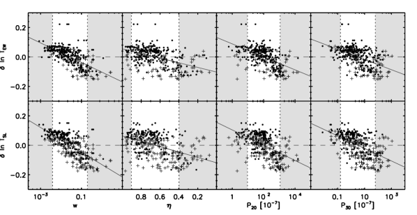
Figure 6.— Relationship between a cluster’s deviation $\delta\ln T_{\rm X}$ from the mean $M$-$T_{\rm X}$ relationship and four measures of substructure: the centroid variation $w$, the axial ratio $\eta$, and the power ratios $P_{20}$ and $P_{30}$. The lower panels are for spectroscopic-like temperature, and the upper ones are for emission-weighted temperature. The light gray bands and vertical dashed lines show the extremes in substructure measurements, with 80% of our clusters falling in the central region between the bands. The black filled circles correspond to clusters above 2 keV, while the plus signs correspond to clusters below 2 keV. Finally, the solid lines indicate the best-fitting linear relationships between our substructure measures and temperature offset, for the above 2 keV sub-sample denoted by the black filled circles.

To further illustrate this point, we have computed an axial ratio value for this cluster for every possible choice of aperture placement. Apertures of radius $R_{500}$ were centered on each and every pixel within the surface-brightness map, provided the aperture so placed does not reach the edge of the map. This procedure generated an axial-ratio “surface” mapping all of the aperture placements to a value of $\eta$. Figure 4 shows the axial-ratio surface for the cluster in Figure 3. For comparison purposes, Figure 5 presents an axial-ratio surface map for a very symmetric, uniform, and apparently relaxed cluster, in which the cluster’s brightness peak reassuringly corresponds to the aperture location that maximizes $\eta$. In contrast, the presence of two peaks in the axial-ratio surface for the asymmetric cluster shows that $\eta$ can sometimes depend strongly on aperture placement. Ideally, we would like to place the aperture on the “center” of this cluster, but the center of an unrelaxed cluster can be difficult to define, meaning that the axial ratio statistic may be likewise ill-defined for such clusters.

3.2. Power Ratio

The power-ratio statistics (Buote & Tsai, 1995; O’Hara et al., 2006) quantify substructure by decomposing the surface-brightness image into a two-dimensional multipole expansion, the terms of which are calculated from the moments of the image, computed within an aperture of radius $R_{\rm ap}$:

$$a_{m}(R_{\rm ap})=\int_{R^{\prime}\leq R_{\rm ap}}\Sigma(\vec{x}^{\prime})(R^{\prime})^{m}\cos m\phi^{\prime}\ d^{2}x^{\prime}$$ (7)

$$b_{m}(R_{\rm ap})=\int_{R^{\prime}\leq R_{\rm ap}}\Sigma(\vec{x}^{\prime})(R^{\prime})^{m}\sin m\phi^{\prime}\ d^{2}x^{\prime}.$$ (8)

The power in terms of order $m$ is then

$$P_{m}=\frac{(a_{m}^{2}+b_{m}^{2})}{2m^{2}R_{\rm ap}^{2m}}.$$ (9)

For $m=0$, the power is given by

$$P_{0}=[a_{0}\ln(R_{\rm ap})]^{2}.$$ (10)

The power ratios $P_{m0}\equiv P_{m}/P_{0}$ are then dimensionless measures of substructure which have differing interpretations. For instance, $P_{10}$ quantifies the degree of balance about some origin and can be used to find the image centroid, $P_{20}$ is related to the ellipticity of the image, and $P_{30}$ is related to the triangularity of the photon distribution. As in the case of the axial ratio computations, we set the aperture radius $R_{\rm ap}$ equal to $R_{500}$. The most appropriate place to center the aperture is at the set of pixel coordinates that minimizes $P_{10}$, which we achieve using a self-annealing algorithm.

3.3. Centroid Variation

The centroid variation statistic $w$ is a measure of the center shift, or “skewness”, of a two-dimensional photon distribution. It is measured for a cluster surface-brightness map in the following way. For a set of surface-brightness levels one finds the centroids of the corresponding isophotal contours and computes the variance in the coordinates of those centroids, scaled to $R_{500}$. Here we select 10 isophotes evenly spaced in $\log I_{\rm X}$ between the minimum and maximum of $I_{\rm X}$ within an aperture of radius $R_{500}$ centered on the brightness peak, so as to adapt to the full dynamic range of surface brightness for different clusters. We employed this adaptive scheme because using one set of isophotes for all clusters tended to ignore important substructure in less massive clusters when they had surface brightness substructure inside $R_{500}$ but outside of the lowest isophote.

3.4. Substructure and Scaling Relationships

Using the quantitative measures of substructure described in the previous section, we can test the significance of the relationship between substructure and temperature offset hinted at in Figure 2. We begin by treating four of our substructure statistics—centroid variation $w$, axial ratio $\eta$, and power ratios $P_{20}$ and $P_{30}$—as different imperfect measurements of an intrinsic degree of substructure $S$. Figure 6 shows the relationship between substructure and a cluster’s deviation $\delta\ln T_{\rm X}$ from the mean $M$-$T_{\rm X}$ relation for each substructure measure. In each case we present results for both the spectroscopic-like temperature $T_{\rm SL}$ and the emission-weighted temperature $T_{\rm EW}$. Note that centroid variation $w$ and the power ratios $P_{20}$ and $P_{30}$ have large dynamic ranges, whereas the axial ratio $\eta$ is always of order unity. We therefore attempt to fit the relationships between $\delta\ln T_{\rm X}$ and the different substructure measures with the following forms:

$$\delta\ln T_{\rm X}=\left\{\begin{array}[]{l}Aw^{\alpha}\\ B+\beta\eta\\ CP_{20}^{\gamma}\\ DP_{30}^{\lambda}\end{array}\right.$$ (11)

To visually indicate where the bulk of our substructure measures lie, Figure 6 has light gray bands covering the extremes, so that 80% of our sample clusters have substructure measures lying between the extremes. The power ratios in our study generally span two decades (in units of $10^{-7}$), from $\sim$2—300 for $P_{20}$ and from $\sim$0.01—10 for $P_{30}$. These ranges are consistent with those of Buote & Tsai (1995), O’Hara et al. (2006), and Jeltema et al. (2007). The measurements of axial ratio in our sample, with 80% of clusters having $\eta$$\sim$0.4—0.95, cover a slightly wider range than do the simulated clusters of O’Hara et al. (2006). Finally, our measurements of centroid variation, with 80% of clusters having $w[R_{500}]$$\sim$0.01—0.1, are again similar to those of O’Hara et al. (2006).

As denoted in Figure 6 by black filled circles, the systems with $T_{\rm X}$ above 2 keV occupy a slightly narrower range of substructure values than the systems below 2 keV, which are denoted by plus signs. For the axial ratio and the power ratios, the variance is 15 to 25 percent larger among the low-temperature systems when compared to the systems with $T_{\rm X}>$ 2 keV. For centroid variation the variance among the low-temperature systems is approximately the same as it is among the high-temperature systems. However, it is not clear that there is a significant correlation between substructure and mass, since the mean substructure values are generally very similar between the low-temperature and high-temperature subsamples. The mean value of the power ratio $P_{30}$ is significantly larger for the low-temperature subsample, however this measure also has the weakest correlation with offsets from the mean $M$-$T_{\rm X}$ relation.

To test whether the low-mass clusters in our sample significantly boost the overall scatter in the $M$-$T_{\rm X}$ relation, we perform a cut at 2 keV and fit this relation both to the whole sample and to the sub-sample above 2 keV. Figure 7 shows the residuals in mass, actual minus predicted, where the predicted mass derives only from the $M$-$T_{\rm X}$ relation. The plus signs indicate clusters whose mass is predicted from an $M$-$T_{\rm X}$ relation derived from all 121 clusters. The black filled circles indicate clusters that are above 2 keV in X-ray temperature, with the mass estimated using the sub-sample $M$-$T_{\rm X}$ relation. There is a negligible reduction in scatter, from 0.127 to 0.124 for $T_{\rm SL}$ and from 0.102 to 0.094 for $T_{\rm EW}$, suggesting that at best only a modest improvement is found in our sample if we remove the low-mass systems. In order to test the degree to which incorporating substructure measures adds to this modest improvement, when we compare mass estimates derived using substructure to those derived only from the $M$-$T_{\rm X}$ relation, we focus on clusters above 2 keV in the rest of our analysis.

Figure 6 shows that for our simulated clusters, a greater amount of measured substructure tends to be associated with “cooler” clusters while less substructure tends to be associated with “hotter” clusters. Also, the centroid variations $w$ are more highly-correlated with $\delta\ln T_{\rm X}$ than are the other substructure parameters. We interpret this to mean that the centroid variation is a better predictor of the offset in the $M$-$T_{\rm X}$ relationship than are the power ratios and the axial ratio, though all four measures appear to be related to the temperature offset. Again, in this figure we denote systems above 2 keV by black filled circles, and systems below 2 keV by plus signs.

Figure 7.— Comparison of mass offset $\delta\ln M$ between true mass and predicted mass, based on the $M(T_{\rm X})$ relation. Plus signs indicate residuals for masses estimated from the $M$-$T_{\rm X}$ relation derived from all 121 clusters, while black filled circles are for masses estimated from the $M$-$T_{\rm X}$ relation for clusters above 2 keV. Upper panels are for spectroscopic-like temperature and lower panels are for emission-weighted temperature. The standard deviations $\sigma$ in the residuals are given in each plot.

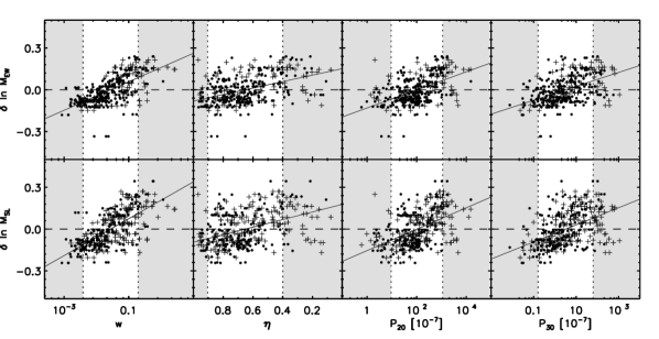
Figure 8.— Relationship between substructure and mass offset $\delta\ln M(T_{\rm X})$ from the mean $M$-$T_{\rm X}$ relationship for the same substructure measures as in Figure 6. The lower panels are for $T_{\rm X}=T_{\rm SL}$, and the upper panels are for $T_{\rm X}=T_{\rm EW}$. As in Figure 6 the solid lines indicate the best-fitting linear relationships to the above 2 keV sub-sample denoted by black filled circles, and the gray bands and vertical dashed lines mark the extremes in substructure between which 80% of our clusters lie. Also as in Figure 6, the plus signs correspond to systems below 2 keV., while the black filled circles correspond to systems above 2 keV.

Correlations between substructure and $\delta\ln T_{\rm X}$ can potentially be exploited to improve on mass estimates of real clusters derived from the mass-temperature relation. Instead of computing the temperature offset at fixed mass, we can determine a substructure-dependent mass offset at fixed temperature and then apply it as a correction to the predicted mass $M_{\rm pred}(T_{\rm X})$ one would derive from the mean $M$-$T_{\rm X}$ relation alone. To assess the prospects for such a correction, based on this sample of simulated clusters, we first define the mass offset from the mean mass-temperature relation to be

$$\delta\ln M(T_{\rm X})=\ln\left[\frac{M}{M_{\rm pred}(T_{\rm X})}\right]\;\;,$$ (12)

where $M$ is the cluster’s actual mass, and examine the correlations between substructure measures and $\delta\ln M$. Figure 8 shows the results. These plots show mass predictions from both the $M$-$T_{\rm SL}$ relation and the $M$-$T_{\rm EW}$ relation. Consistent with our analysis of $\delta\ln T_{\rm X}$, the centroid variation $w$ appears to be a more effective predictor of the mass offset $\delta\ln M(T_{\rm X})$. Nonetheless, all four measures of substructure appear to be correlated with mass offset.

Figure 9.— Comparison of mass offset $\delta\ln M$ between true mass and predicted mass, based on the $M(T_{\rm X})$ relation (open circles) and the $M(T_{\rm X},S)$ relation (filled circles). Upper panels are for $T_{\rm SL}$ and lower panels are for $T_{\rm EW}$. The standard deviations $\sigma$ in the residuals are given in each plot.

In order to incorporate a substructure correction into the mass-temperature relation, we perform a multiple regression, fitting our simulated clusters’ mass, temperature, and substructure data to the form,

$$\log M_{\rm pred}(T_{\rm X},S)=\log M_{0}+\alpha\log T_{\rm X}+\beta S,$$ (13)

where $S$ represents one of the following substructure measures: $\eta$, $\log w$, $\log P_{20}$, or $\log P_{30}$. This fit gives us a substructure-corrected mass prediction $M_{\rm pred}(T_{\rm X},S)$ for each substructure measure, and we can assess the effectiveness of that correction by measuring the dispersion of the substructure-corrected mass offset

$$\delta\ln M(T_{\rm X},S)=\ln\left[\frac{M}{M_{\rm pred}(T_{\rm X},S)}\right]\;\;,$$ (14)

between the revised prediction and the true cluster mass.

Figure 9 shows the results of that test. Open circles in each panel indicate mass offsets $\delta\ln M(T_{\rm X})$ without substructure corrections, which have a standard deviation $\sigma_{M(T)}$. Filled circles indicate mass offsets $\delta\ln M(T_{\rm X},S)$ with substructure corrections, which have a standard deviation $\sigma_{M(T,S)}$. The upper set of panels shows results for $T_{\rm SL}$, and the lower set is for $T_{\rm EW}$. In each case, incorporating a substructure correction to the mass-temperature relation reduces the scatter, yielding more accurate mass estimates. The centroid variation corrections are the most effective, reducing the scatter in mass from 0.124 to 0.085 in the $M$-$T_{\rm SL}$ relation and from 0.094 to 0.072 in the $M$-$T_{\rm EW}$ relation, though admittedly this is again a modest improvement. Although non-negligible structure correlates significantly with offsets in the $M$-$T_{\rm X}$ plane, apparently it does so with substantial scatter. This scatter may be partly due to projection effects, in which line-of-sight mergers are discounted by the measures of substructure and may dilute their corrective power (Jeltema et al., 2007).

Lastly, Figure 10 shows the results for a similar analysis to that of Figure 9, except that in this case we have excised a region of radius 0.15$R_{500}$ around the center of each cluster and recomputed $T_{\rm EW}$. We do this to test whether offset in temperature, whose correlation with substructure is the basis of our correction scheme, stems from a potentially unrealistic feature, which is that the cores of many real clusters have temperature profiles that decline at larger radii than occurs in simulated clusters. As in Figure 9, we restrict our analysis to clusters above 2 keV. After doing this test, for $T_{\rm EW}$ excising the core actually increases the scatter in $M$-$T_{\rm X}$ from 0.094 to 0.106. It may be that by removing the bright central region, the average temperature becomes more sensitive to structure outside the core. Also, this figure shows that the effect of incorporating substructure measurements into the mass-estimates is still present. The scatter is reduced to 0.075 for $w$, 0.093 for $\eta$, 0.090 for $P_{20}$ and 0.094 for $P_{30}$. Figure 10 summarizes the results of this test, which support the conclusion that the reduction in scatter we realize using substructure is a real effect and not an artifact of known defects in the simulations.

3.5. Comparisons with Other Substructure Studies

O’Hara et al. (2006) examined the relationship between galaxy cluster substructure and X-ray scaling relationships, including the $M$-$T_{\rm X}$ relation, using both a flux-limited sample of nearby clusters and a sample of simulated clusters, and found a greater amount scatter among the more relaxed clusters in their observed sample. Contrasting that result they also found a greater amount of scatter among the more disrupted clusters in their simulation sample, though they characterize the evidence for this second result to be weak. Finally, they see no evidence in either sample for more disrupted clusters to be below the mean, and the more relaxed clusters to be above. One difference between our study and theirs is the presence of radiative cooling and supernova feedback in the simulation that produced our cluster sample. Also, the focus of our work is different from theirs in that we concentrate on the degree of correlation between the amount of substructure and the size and direction of the offset from the mean relation. We do find significant evidence of this correlation, such that relaxed clusters are hotter than expected given their mass. We also test, as best we can given our simulation sample, the hypothesis that substructure can be used to improve mass estimates derived from the ICM X-ray temperature. It is possible that our detection of a correlation between substructure and temperature offset arises from the additional physics in our simulated clusters, since when radiative cooling is included, cool lumps may be better preserved than in simulations that don’t include cooling.

Figure 10.— Comparison of mass offset $\delta\ln M$ between true mass and predicted mass, based on the $M(T_{\rm X})$ relation (open circles) and the $M(T_{\rm X},S)$ relation (filled circles). These results are for are for $T_{\rm EW}$, with the central 0.15 $R_{500}$ region removed both from the average temperature and from the substructure measures. The standard deviations $\sigma$ in the residuals are given in each plot.

Our results are in agreement with Valdarnini (2006), who examined substructure in clusters simulated with cooling and feedback and found that unrelaxed clusters, identified with a larger power ratio $P_{30}$, have spectral-fit temperatures biased low relative to the mass-weighted temperatures. This trend aligns with our finding that the spectroscopic-like temperature $T_{\rm SL}$ is lower than the best-fit temperature at fixed mass for clusters with larger power ratios $P_{20}$ and $P_{30}$. However, Valdarnini (2006) did not investigate the effectiveness of substructure measures in reducing scatter in the mass-temperature relation.

Our results are also in agreement with some of the results of Jeltema et al. (2007), who have recently investigated correlations between substructure and offsets in mass predictions in simulated clusters. They found that measuring cluster structure is an effective way to correct masses estimated using the assumption of hydrostatic equilibrium, which tend to be underestimates. Our findings support these results, given that we find substructure can be used to correct masses estimated directly from the $M$-$T_{\rm X}$ relationship. There also are differences between our findings and theirs. They report that the $M$-$T_{\rm X}$ relation for their simulation sample shows no dependence on structure, whereas the clusters in our sample exhibit offsets that correlate with the degree of substructure. One possibility is that these differences stem from differences in the simulations’ feedback mechanisms. Another possibility is that some of the offset we observe derives from enhanced temperatures in simulations with radiative cooling. As we describe in section 3, we perform a test in which we estimate $T_{\rm EW}$ using projected surface-brightness and temperature maps, in order to remove the core regions from our analysis, but this may be less effective than properly excising the cores in the simulations, as Jeltema et al. (2007) have done.

Kravtsov et al. (2006) also looked at the relationship that cluster structure has to the $M$-$T_{\rm X}$ relation in simulated clusters, to show that the sensitivity of mass proxies $Y_{X}$ and $Y_{SZ}$ to substructure is not very strong. They divided their sample into unrelaxed and relaxed subsamples, based on the presence or absence of multiple peaks in the surface-brightness maps of clusters, and found the normalization of the $M$-$T_{\rm X}$ relation to be biased to cooler temperatures for the unrelaxed systems. Other workers also have looked at the relationship between the $M$-$T_{\rm X}$ relation and substructure, as reflected in the X-ray spectral properties. Mathiesen & Evrard (2001) have examined the ratio of X-ray spectral-fit temperatures in hard and full bandpasses for an ensemble of simulated clusters, and found it to be a way of quantifying the dynamical state of a cluster. We consider our approach of using surface-brightness morphology information to be complementary to theirs. More recently, Kay et al. (2007) performed an interesting analysis on another large-volume simulation sample, using as substructure metrics the centroid variation and measures of concentration to report evolution in the luminosity-temperature relationship. Specifically, they report that the more irregular clusters in their sample lie above the mean $M$-$T_{\rm X}$ relation (i.e., they are cooler than average), for the spectroscopic-like temperature $T_{\rm SL}$.

4. Summary

Using a sample of galaxy clusters simulated with cooling and feedback, we investigated three substructure statistics and their correlations with temperature and mass offsets from mean scaling relations in the $M$-$T_{\rm X}$ plane. First, we showed that the substructure statistics $w$, $\eta$, $P_{20}$ and $P_{30}$ all correlate significantly with $\delta\ln T_{\rm X}$, though with non-negligible scatter. In all cases this scatter is larger for $\delta\ln$ $T_{\rm SL}$ than it is for $\delta\ln$ $T_{\rm EW}$. Next, we considered the possibility that $M$-$T_{\rm X}$ scatter is driven by low-mass clusters. We tested the degree to which scatter can be reduced by filtering out these systems. This consisted of performing a cut at 2 keV, for which we saw that it yielded a modest improvement in mass estimates. To see whether incorporating substructure could refine these mass estimates, we first showed that $w$, $\eta$, $P_{20}$, and $P_{30}$ correlate significantly with the difference $\delta\ln M$ between masses predicted from the mean $M(T_{\rm X})$ relation and the true cluster masses, with non-negligible scatter that again is less for $M(T_{\rm EW})$ than it is for $M(T_{\rm SL})$. Then we adopted a full three-parameter model, $M$-$T_{\rm X}$-$S$, which includes substructure information $S$ estimated using $w$, $\eta$, $P_{20}$, and $P_{30}$. Scatter about the basic two-parameter $M$-$T_{\rm EW}$ relation was 0.094. Including substructure as a third parameter reduced the scatter to 0.072 for centroid variation, 0.084 for axial ratio, 0.081 for $P_{20}$, and 0.084 for $P_{30}$. Scatter about the basic two-parameter $M$-$T_{\rm SL}$ relation was 0.124, and including substructure as a third parameter reduced the scatter to 0.085 for centroid variation, 0.112 for axial ratio, 0.110 for $P_{20}$, and 0.108 for $P_{30}$. As one last test, and to increase our confidence that our substructure measures are not relying on potentially non-physical core structure in the simulations, we also repeated the comparison of mass-estimates for $T_{\rm EW}$, with the core regions of the clusters excised. First, removing the core slightly increased the scatter in $M$-$T_{\rm X}$  possibly by making the average temperature more sensitive to structure outside the core. Second, even with the cores removed the improvement in mass-estimates obtained using substructure information remains. Based on these results, it appears that centroid variation is the best substructure statistic to use when including a substructure correction in the $M$-$T_{\rm EW}$ relation. However, the correlations we have found in this sample of simulated clusters might not hold in samples of real clusters, because relaxed clusters in the real universe tend to have cooler cores than our simulated clusters do.

References

- Borgani et al. (2004) Borgani, S., Murante, G., Springel, V., Diaferio, A., Dolag, K., Moscardini, L., Tormen, G., Tornatore, L., & Tozzi, P. 2004, MNRAS, 348, 1078
- Buote & Tsai (1995) Buote, D. A., & Tsai, J. C. 1995, ApJ, 452, 522
- Evrard et al. (2007) Evrard, A. E., Bialek, J., Busha, M., White, M., Habib, S., Heitmann, K., Warren, M., Rasia, E., Tormen, G., Moscardini, L., Power, C., Jenkins, A. R., Gao, L., Frenk, C. S., Springel, V., White, S. D. M., & Diemand, J. 2007, ArXiv Astrophysics e-prints
- Evrard et al. (1993) Evrard, A. E., Mohr, J. J., Fabricant, D. G., & Geller, M. J. 1993, ApJ, 419, L9+
- Fabian et al. (1994) Fabian, A. C., Crawford, C. S., Edge, A. C., & Mushotzky, R. F. 1994, MNRAS, 267, 779
- Hu (2003) Hu, W. 2003, Phys. Rev. D, 67, 081304
- Jeltema et al. (2007) Jeltema, T. E., Hallman, E. J., Burns, J. O., & Motl, P. M. 2007, ArXiv e-prints, 708
- Kaiser (1986) Kaiser, N. 1986, MNRAS, 222, 323
- Kay et al. (2007) Kay, S. T., da Silva, A. C., Aghanim, N., Blanchard, A., Liddle, A. R., Puget, J.-L., Sadat, R., & Thomas, P. A. 2007, MNRAS, 377, 317
- Kravtsov et al. (2006) Kravtsov, A. V., Vikhlinin, A., & Nagai, D. 2006, ApJ, 650, 128
- Levine et al. (2002) Levine, E. S., Schulz, A. E., & White, M. 2002, ApJ, 577, 569
- Lima & Hu (2005) Lima, M., & Hu, W. 2005, Phys. Rev. D, 72, 043006
- Majumdar & Mohr (2004) Majumdar, S., & Mohr, J. J. 2004, ApJ, 613, 41
- Markevitch (1998) Markevitch, M. 1998, ApJ, 504, 27
- Mathiesen & Evrard (2001) Mathiesen, B. F., & Evrard, A. E. 2001, ApJ, 546, 100
- Mazzotta et al. (2004) Mazzotta, P., Rasia, E., Moscardini, L., & Tormen, G. 2004, ArXiv Astrophysics e-prints
- McCarthy et al. (2004) McCarthy, I. G., Balogh, M. L., Babul, A., Poole, G. B., & Horner, D. J. 2004, ApJ, 613, 811
- Nagai et al. (2007) Nagai, D., Kravtsov, A. V., & Vikhlinin, A. 2007, ApJ, 668, 1
- Navarro et al. (1995) Navarro, J. F., Frenk, C. S., & White, S. D. M. 1995, MNRAS, 275, 720
- O’Hara et al. (2006) O’Hara, T. B., Mohr, J. J., Bialek, J. J., & Evrard, A. E. 2006, ApJ, 639, 64
- Pearce et al. (1994) Pearce, F. R., Thomas, P. A., & Couchman, H. M. P. 1994, MNRAS, 268, 953
- Phillips (1993) Phillips, M. M. 1993, ApJ, 413, L105
- Poole et al. (2007) Poole, G. B., Babul, A., McCarthy, I. G., Fardal, M. A., Bildfell, C. J., Quinn, T., & Mahdavi, A. 2007, MNRAS, 380, 437
- Riess et al. (1996) Riess, A. G., Press, W. H., & Kirshner, R. P. 1996, ApJ, 473, 88
- Saro et al. (2006) Saro, A., Borgani, S., Tornatore, L., Dolag, K., Murante, G., Biviano, A., Calura, F., & Charlot, S. 2006, MNRAS, 373, 397
- Springel (2005) Springel, V. 2005, MNRAS, 364, 1105
- Tormen (1997) Tormen, G. 1997, MNRAS, 290, 411
- Tornatore et al. (2003) Tornatore, L., Borgani, S., Springel, V., Matteucci, F., Menci, N., & Murante, G. 2003, MNRAS, 342, 1025
- Valdarnini (2006) Valdarnini, R. 2006, New Astronomy, 12, 71
- Vikhlinin (2006) Vikhlinin, A. 2006, ApJ, 640, 710
- Voit (2005) Voit, G. M. 2005, Phys. Rev. D, 77, 207
- Voit et al. (2002) Voit, G. M., Bryan, G. L., Balogh, M. L., & Bower, R. G. 2002, ApJ, 576, 601
- Wang & Steinhardt (1998) Wang, L., & Steinhardt, P. J. 1998, ApJ, 508, 483