Electric displacement as the fundamental variable in electronic-structure calculations

Abstract

Finite-field calculations in periodic insulators are technically and conceptually challenging, due to fundamental problems in defining polarization in extended solids. While significant progress has been made recently with the establishment of techniques to fix the electric field $\bm{\mathcal{E}}$ or the macroscopic polarization $\mathbf{P}$ in first-principles calculations, both methods lack the ease of use and conceptual clarity of standard zero-field calculations. Here we develop a new formalism in which the electric displacement $\mathbf{D}$, rather than $\bm{\mathcal{E}}$ or $\mathbf{P}$, is the fundamental electrical variable. Fixing $\mathbf{D}$ has the intuitive interpretation of imposing open-circuit electrical boundary conditions, which is particularly useful in studying ferroelectric systems. Furthermore, the analogy to open-circuit capacitors suggests an appealing reformulation in terms of free charges and potentials, which dramatically simplifies the treatment of stresses and strains. Using PbTiO₃ as an example, we show that our technique allows full control over the electrical variables within the density functional formalism.

The development of the modern theory of polarization King-Smith/Vanderbilt:1993 has fueled exciting progress in the theory of the ferroelectric state. Many properties that could previously be inferred only at a very qualitative level can now be computed with quantum-mechanical accuracy within first-principles density-functional theory. Early ab-initio studies focused on bulk ferroelectric crystals, elucidating the delicate balance between covalency and electrostatics that gives rise to ferroelectricity. Over time, these methods were extended to treat the effects of external parameters such as strains or electric fields Souza/Iniguez/Vanderbilt:2002 ; Umari/Pasquarello:2002 . Of particular note is the recent introduction by Diéguez and Vanderbilt Dieguez/Vanderbilt:2006 of a method for performing calculations at fixed macroscopic polarization $\mathbf{P}$. The ability to compute crystal properties from first principles as a function of $\mathbf{P}$ provides an an intuitive and appealing link to Landau-Devonshire and related semiempirical theories in which $\mathbf{P}$ serves as an order parameter.

Despite its obvious appeal, however, the constrained-$\mathbf{P}$ method has found limited practical application to date. One reason for this is that the procedure to enforce a constant $\mathbf{P}$ during the electronic self-consistency cycle is relatively involved; this hampers the study of complex heterostructures with large supercells, where computational efficiency is crucial. There are also physical reasons. In particular, fixing $\mathbf{P}$ does not correspond to experimentally realizable electrical boundary conditions (Fig. 1). Moreover, in an inhomogeneous heterostructure, the local polarization can vary from one layer to another, and its average is therefore best regarded as a derived, not a fundamental, quantity. In the following we show that considering $\mathbf{D}$ as the fundamental electrical variable overcomes these physical limitations, and that constraining $\mathbf{D}$ rather than $\mathbf{P}$ leads to a simpler implementation.

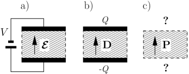
Figure 1: Electrical boundary conditions within different methods. a) The fixed-$\bm{\mathcal{E}}$ method corresponds to adopting closed-circuit boundary conditions with a constant applied bias $V$. b) Constraining $\mathbf{D}$ corresponds to a capacitor in open-circuit conditions with a fixed value of the free charge $Q$ on the plates. c) constraining $\mathbf{P}$ does not correspond to a clear experimental set-up.

Formalism. We consider a periodic insulating crystal defined by three primitive translation vectors $\mathbf{a}_{i}$, with $\Omega$ the unit cell volume, and we introduce the new functional

$$U(\mathbf{D},v)=E_{\rm KS}(v)+\frac{\Omega}{8\pi}[\mathbf{D}-4\pi\mathbf{P}(v)]^{2}\;.$$ (1)

$U(\mathbf{D},v)$ depends directly on an external vector parameter $\mathbf{D}$, and indirectly on the internal (ionic and electronic) coordinates $v$ through the Kohn-Sham energy $E_{\rm KS}$ and the Berry-phase polarization $\mathbf{P}$ King-Smith/Vanderbilt:1993 . (For the moment we fix the lattice vectors; strains will be discussed shortly.) The minimum of $U$ at fixed $\mathbf{D}$ is given by the stationary point where all the gradients with respect to $v$ vanish,

$$\frac{\partial U}{\partial v}\Big{|}_{\mathbf{D}}=\frac{\partial E_{\rm KS}}{\partial v}-\Omega\,(\mathbf{D}-4\pi\mathbf{P})\cdot\frac{\partial\mathbf{P}}{\partial v}=0\;.$$ (2)

Comparing with the fixed-$\bm{\mathcal{E}}$ approach of Ref. Souza/Iniguez/Vanderbilt:2002 ; Umari/Pasquarello:2002 in which the electric enthalpy $\mathcal{F}$ is given by

$$\mathcal{F}(\bm{\mathcal{E}},v)=E_{\rm KS}(v)-\Omega\,\bm{\mathcal{E}}\cdot\mathbf{P}(v)\;,$$ (3)

we see that

$$\frac{\partial\mathcal{F}}{\partial v}\Big{|}_{\bm{\mathcal{E}}}=\frac{\partial U}{\partial v}\Big{|}_{\mathbf{D}}$$ (4)

provided that we set $\bm{\mathcal{E}}=\mathbf{D}-4\pi\mathbf{P}$. We thus discover that $\mathbf{D}=\bm{\mathcal{E}}+4\pi\mathbf{P}$ is the macroscopic electric displacement field. The functional in Eq. (1) takes the form $U=E_{\rm KS}+(\Omega/8\pi)\,\bm{\mathcal{E}}^{2}$, which is the correct expression for the internal energy of a periodic crystal when a uniform external field is present (details are given in Supplementary Section 2.4). Eq. (1) thus provides a framework for finding the minimum of the internal energy $U(\mathbf{D})$ with respect to all internal degrees of freedom at specified electric displacement $\mathbf{D}$. This is the essence of our constrained-$\mathbf{D}$ method.

As a consequence of Eq. (4), the method is analogous to a standard finite-$\mathcal{E}$-field calculation Souza/Iniguez/Vanderbilt:2002 ; Umari/Pasquarello:2002 . In particular, the Hellmann-Feynman forces are computed in the same way. The only difference is that the value of $\bm{\mathcal{E}}$, instead of being kept constant, is updated at every iteration until the target value of $\mathbf{D}$ is obtained at the end of the self-consistency cycle (or ionic relaxation). This implies that the implementation and use of the constrained-$\mathbf{D}$ method in an existing finite-$\cal E$-field code is immediate; in our case it required the modification of two lines of code only.

The effect of constraining $\mathbf{D}$, rather than $\bm{\mathcal{E}}$, essentially corresponds to the imposition of longitudinal, rather than transverse, electrical boundary conditions. For example, as we shall see below, the phonon frequencies obtained from the force-constant matrix computed at fixed $\mathbf{D}$ are the longitudinal optical (LO) ones, while the usual approach yields instead the transverse optical (TO) frequencies. Furthermore, the longitudinal electrical boundary conditions are appropriate to the physical realization of an open-circuit capacitor with fixed free charge on the plates, while the usual approach applies to a closed-circuit one with a fixed voltage across the plates (Fig. 1).

Stress tensor. This analogy with an open-circuit capacitor suggests an intuitive strategy for deriving the stress tensor, a quantity that plays a central role in piezoelectric materials. In particular, the electrode of an isolated open-circuit capacitor cannot exchange free charge with the environment. This suggests that the flux of the vector field $\mathbf{D}$ through the three independent facets of the primitive unit cell should remain constant under an applied strain. These fluxes are $\mathbf{a}_{i}\times\mathbf{a}_{j}\cdot\mathbf{D}=\Omega\,\mathbf{b}_{i}\cdot\mathbf{D}$, where the $\mathbf{b}_{i}$ are duals ($\mathbf{a}_{i}\cdot\mathbf{b}_{j}=\delta_{ij}$) differing by a factor of $2\pi$ from the conventional reciprocal lattice vectors. We then rewrite the functionals in terms of the “internal” or “reduced” variables $d_{i}=(\Omega/4\pi)\,\mathbf{b}_{i}\cdot\mathbf{D}$. It is also useful to define the reduced polarization $p_{i}=\Omega\,\mathbf{b}_{i}\cdot\mathbf{P}$ and the “dual” reduced electric field $\bar{\varepsilon}_{i}=\mathbf{a}_{i}\cdot\mathcal{E}$. Additional details are provided in the Supplementary Section 4.

By Gauss’s law, $d_{i}=-Q_{i}$, where the $Q_{i}$ are the free charges per surface unit cell located on the cell face normal to $\mathbf{b}_{i}$. With these definitions, the internal energy can be rewritten as

$$U(\{d\})=E_{\rm KS}+\frac{2\pi}{\Omega}\sum_{ij}\big{(}d_{i}-p_{i}\big{)}\,g_{ij}\,\big{(}d_{j}-p_{j}\big{)}$$ (5)

where we have introduced the metric tensor $g_{ij}=\mathbf{a}_{i}\cdot\mathbf{a}_{j}$. We then define the fixed-$\{d\}$ stress tensor as

$$\sigma_{\mu\nu}=\frac{1}{\Omega}\left(\frac{dU}{d\eta_{\mu\nu}}\right)_{\{d\}}$$ (6)

where $\eta_{\mu\nu}$ is the strain tensor. By a Hellmann-Feynman argument (see Supplementary Section 4.3) the total derivative in Eq. (6) can be replaced by a partial derivative. Using $dg_{ij}/d\eta_{\mu\nu}=2a_{iu}a_{jv}$, we find

$$\sigma_{\mu\nu}=\sigma_{\mu\nu}^{\rm KS}+\sigma_{\mu\nu}^{\rm Max}+\sigma_{\mu\nu}^{\rm aug}\,,$$ (7)

where $\sigma_{\mu\nu}^{\rm KS}$ is the standard zero-field expression,

$$\sigma_{\mu\nu}^{\rm Max}=\frac{2\mathcal{E}_{\mu}\mathcal{E}_{\nu}-\delta_{\mu\nu}\mathcal{E}^{2}}{8\pi}$$ (8)

is the Maxwell stress tensor (which originates from the derivative acting on $g_{ij}$ and $\Omega^{-1}$), and

$$\sigma_{\mu\nu}^{\rm aug}=-\frac{1}{\Omega}\sum_{i}\,\bar{\varepsilon}_{i}\,\frac{\partial p_{i}}{\partial\eta_{\mu\nu}}\,$$ (9)

is the “augmented” part. If the internal variables $v$ are chosen as reduced atomic coordinates and plane-wave coefficients in a norm-conserving pseudopotential context, neither the ionic nor the Berry-phase component of $p_{i}$ has any explicit dependence on strain, and $\sigma_{\mu\nu}^{\rm aug}$ vanishes. The name thus refers to the fact that $\sigma_{\mu\nu}^{\rm aug}$ is nonzero only in ultrasoft pseudopotential Vanderbilt:1990 and projector augmented-wave Bloechl:1994 contexts.

We note that, as a consequence of fixing the reduced variables $d_{i}$ rather than the Cartesian $\mathbf{D}$, the proper treatment of piezoelectric effects Vanderbilt:2000 ; Wu/Vanderbilt/Hamann:2005 is automatically enforced. This formal simplification allows for an enhanced flexibility in the simultaneous treatment of electric fields and strains. For example, it is possible to introduce a rigorous constant-pressure enthalpy by simply defining

$$U^{\pi}(d)=\min_{\eta}[U(d,\eta)-\pi\Omega]\,,$$ (10)

where $\pi$ is the external pressure and $\Omega$ is the cell volume. We will demonstrate the use of this strategy in the application to PbTiO₃.

Legendre transformation. The transformation from variables $\mathbf{D}$ to variables $\bm{\mathcal{E}}$ can be regarded as part of a Legendre transformation. We spell out this connection here, working instead with reduced variables $(d_{1},d_{2},d_{3})$ and $(\bar{\varepsilon}_{1},\bar{\varepsilon}_{2},\bar{\varepsilon}_{3})$. First, we note that

$$\frac{dU}{dd_{i}}=\frac{\partial U}{\partial d_{i}}=\bar{\varepsilon}_{i}\,.$$ (11)

Recall that $\bar{\varepsilon}_{i}=\mathbf{a}_{i}\cdot\bm{\mathcal{E}}$, so that $-\bar{\varepsilon}_{i}$ is just the potential step $V_{i}$ encountered while moving along lattice vector $\mathbf{a}_{i}$, while $Q_{i}$ is just the free charge on cell face $i$. Thus, when the system undergoes a small change at fixed $(\bar{\varepsilon}_{1},\bar{\varepsilon}_{2},\bar{\varepsilon}_{3})$, the work done by the battery is $-\sum_{i}V_{i}\,dQ_{i}=-\sum_{i}\bar{\varepsilon}_{i}\,dd_{i}$. We therefore define

$$\tilde{\mathcal{F}}(\bar{\varepsilon}_{1},\bar{\varepsilon}_{2},\bar{\varepsilon}_{3})=\min_{d_{1},d_{2},d_{3}}\big{[}U(d_{1},d_{2},d_{3})-\sum_{i}\bar{\varepsilon}_{i}\,d_{i}\big{]},$$ (12)

where the potentials $\bar{\varepsilon}_{i}$ have become the new independent variables and $d_{i}$ are now implicit in the minimum condition. The energy functionals $U(\{d_{i}\})$ and $\tilde{\mathcal{F}}(\{\bar{\varepsilon}_{i}\})$ thus form a Legendre-transformation pair.

All the gradients with respect to the internal and strain degrees of freedom are preserved by the Legendre transformation and need not be rederived for $\tilde{\mathcal{F}}$. The physical electrical boundary conditions, however, have changed back to the closed-circuit case. It is therefore natural to expect the functional $\tilde{\mathcal{F}}$ to be closely related to the fixed-$\bm{\mathcal{E}}$ enthalpy $\mathcal{F}$ of Eq. (3). Indeed, it is straightforward to show that

$$\tilde{\mathcal{F}}=U-\frac{\Omega}{4\pi}\mathcal{E}\cdot\mathbf{D}=\mathcal{F}-\frac{\Omega}{8\pi}\mathcal{E}^{2}\;.$$ (13)

At fixed strain and $\bar{\varepsilon}_{i}$, the $\Omega\mathcal{E}^{2}/8\pi$ term is constant, and thus does not contribute to the gradients with respect to the internal variables, consistent with Eq. (4). However, the stress derived from $\mathcal{F}$ differs from the one derived from $\tilde{\mathcal{F}}$ by the Maxwell term $\sigma_{\mu\nu}^{\rm Max}$, which is absent in $\mathcal{F}$ (details of the derivation are provided in Supplementary Section 4.3). Although the Maxwell stress is tiny on the scale of typical first-principles calculations (e.g. $10^{8}$ V/m produces a pressure of $44.3$ KPa), for reasons of formal consistency we encourage the use of $\tilde{\mathcal{F}}$ in place of $\mathcal{F}$ in future works.

Partial Legendre transformations. It is also possible to define hybrid thermodynamic functionals via partial Legendre transformations that act only on one or two of the three electrical degrees of freedom. Of most interest is the case of two fixed $V$ and one fixed $Q$, i.e., functions of variables $(\bar{\varepsilon}_{1},\bar{\varepsilon}_{2},d_{3})$. The special direction is denoted by unit vector $\hat{\mathbf{q}}$ which is along direction $\mathbf{b}_{3}$. When $\bar{\varepsilon}_{1}=\bar{\varepsilon}_{2}=0$, this applies to two common experimental situations: the case of an insulating film sandwiched in the $\hat{\mathbf{q}}$ direction between parallel electrodes in open-circuit boundary conditions, and the case of a long-wavelength LO phonon of wavevector $\mathbf{q}$ where the $\mathbf{q}\rightarrow 0$ limit is taken along direction $\hat{\mathbf{q}}$.

This latter case of LO phonons exemplifies the physical interpretation of our method and its usefulness. While the gradients of $U$ and its partially Legendre-transformed partner are identical, the force constant matrices, which are second derivatives, are not. Indeed, the force-constant matrices are found to differ by

$$\Delta K_{I\alpha,J\beta}=\frac{4\pi}{\Omega}\,\frac{(\mathbf{Z}_{I}\cdot\hat{\mathbf{q}})_{\alpha}(\mathbf{Z}_{J}\cdot\hat{\mathbf{q}})_{\beta}}{\hat{\mathbf{q}}\cdot\mathbf{\epsilon}_{\infty}\cdot\hat{\mathbf{q}}}\;,$$ (14)

where $I\alpha$ labels the atom $I$ and its displacement direction $\alpha$, $\mathbf{Z}_{I\alpha}$ is the corresponding dynamical charge, and $\mathbf{\epsilon}_{\infty}$ is the purely electronic dielectric tensor. This is readily identified as the non-analytic contribution to the LO-TO splitting of a phonon of small wavevector $\mathbf{q}$ in the theory of lattice dynamics Baroni/deGironcoli/DalCorso:2001 . This demonstrates that the lattice dynamical-properties of a given insulating crystal within our fixed-$D$ method are fully consistent with what should be expected from a change in the electrical boundary conditions from transverse to longitudinal.

Dielectric tensor and linear response. This scheme lends itself naturally to the perturbative linear-response analysis of the second derivatives of the internal energy as described in Ref. Wu/Vanderbilt/Hamann:2005 , with two important differences. First, in our scheme the derivatives at constant $\mathbf{D}$ become the elementary tensors, while the derivatives at constant $\bm{\mathcal{E}}$ are “second-level” quantities; this is an advantage, since using $\mathbf{D}$ as independent variable is very convenient in ferroelectric systems. Second, the use of the reduced field variables $d_{i}$ and $\bar{\varepsilon}_{i}$ in place of the macroscopic vector fields $\mathbf{P}$ and $\bm{\mathcal{E}}$ makes the discussion of strains under an applied field much more rigorous and intuitive.

As an example of the relationship between constrained-$\bar{\varepsilon}$ and constrained-$d$ tensors it is useful to introduce the inverse capacitance, $\gamma=C^{-1}$, in matrix form as

$$\gamma_{ij}=\frac{d^{2}U}{dd_{i}dd_{j}}\;.$$ (15)

Incidentally, while this expression is fully general and well-defined in the non-linear regime, for the special case of a linear medium we can write

$$U=U_{0}+\frac{1}{2}\sum_{ij}\gamma_{ij}\,Q_{i}\,Q_{j},$$ (16)

which generalizes the textbook formula $U=Q^{2}/2C$ to the case of three mutually coupled capacitors. It can be shown that the same information can be obtained within the constrained-$\bar{\varepsilon}$ approach by means of the relationship

$$(\gamma^{-1})_{ij}=\frac{d^{2}\tilde{\mathcal{F}}}{d\bar{\varepsilon}_{i}d\bar{\varepsilon}_{j}}\;.$$ (17)

The matrix $\gamma_{ij}$ can be thought of a “reduced” representation of the macroscopic dielectric tensor,

$$(\epsilon^{-1})_{\alpha\beta}=\frac{\Omega}{4\pi}\sum_{i,j}\gamma_{ij}\,b_{i,\alpha}\,b_{j,\beta}\;,$$ (18)

or equivalently

$$\epsilon_{\alpha\beta}=\frac{4\pi}{\Omega}\sum_{i,j}(\gamma^{-1})_{ij}\,a_{i,\alpha}\,a_{j,\beta}\;.$$ (19)

We will consider, in addition to the total static capacitance above, the closely related frozen-strain $\gamma^{\eta}_{ij}$ and frozen-ion $\gamma^{\infty}_{ij}$ tensors. The remainder of the response functions discussed in Ref. Wu/Vanderbilt/Hamann:2005 can be similarly defined in terms of the second derivatives of $U(\{d\},u,\eta)$.

Applications. In the following we illustrate our method by computing the electrical equation of state of a prototypical ferroelectric material, PbTiO₃. Our calculations are performed within the local-density approximation Perdew/Wang:1992 (LDA) of density-functional theory using norm-conserving troullier pseudopotentials and a planewave cutoff of 150 Ry. The tetragonal unit cell contains one formula unit, and a $6\times 6\times 6$ Monkhorst and Pack Monkhorst/Pack:1976 grid is used to sample the Brillouin zone. The finite electric field is applied through a Wannier-based real-space technique Stengel/Spaldin:2007 , which converges quickly as a function of $k$-point mesh resolution Stengel/Spaldin:2005 ; indeed, tests made with finer meshes showed no differences within numerical accuracy. We obtain an equilibrium lattice constant of $a$=3.879 Å for cubic paraelectric PbTiO₃, in line with values previously reported in the literature. Due to the tetragonal symmetry, the state of the system is fully determined by six parameters: the electric displacement $d$, the cell parameters $a$ and $c$, and three internal coordinates describing relative displacements along $z$.

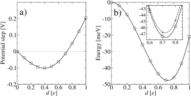
Figure 2: Potential step and internal energy as a function of $d$. Symbols, calculated using constrained-$\mathbf{D}$ method: (a) reduced electric field $\bar{\varepsilon}$ (squares); (b) internal energy $U$ (circles). Solid curves: (a) numerical cubic spline fit to the symbols; (b) numerical integral of the spline fit in (a). Inset: enlargement near the minimum, also showing magnitude of the error made if Pulay stresses are neglected (dashed curve).

Starting from the relaxed cubic structure in zero field, we calculate the equilibrium state for ten evenly spaced values of the reduced displacement $d$, ranging from $d$=0.1 $e$ to $d$=1.0 $e$ (where $-e$ is the electron charge), and relaxing all the structural variables at each $d$ value. We set a stringent accuracy threshold of $10^{-5}$ Ha/bohr for atomic forces and $10^{-7}$ Ha/bohr³ for stresses. First we check the internal consistency of the formalism by verifying that our calculated potential drop $\bar{\varepsilon}$ coincides with the numerical derivative of $U$ with respect to $d$ as expected from Eq. (11). The comparison is shown in Fig. 2, where the discrepancies, of order 10^-6 Ha, are not even visible. This confirms the internal consistency of the formalism and the high numerical accuracy of the calculations. The minimum in Fig. 2 (b) [which coincides with the zero-crossing in (a)] at $d=0.725\,e$ corresponds to a spontaneous polarization of $P_{\rm s}=0.78\,$C/m².

We note that this comparison is sensitive to the Pulay stress, even in the present case where our conservative choice of the plane-wave cutoff makes this error as small as $\pi_{P}$ = 82 MPa. Neglecting such error corresponds to applying a spurious hydrostatic pressure of $-\pi_{P}$, which leads to a discrepancy between the integrated potential (dashed curve in the inset of Fig. 2) and the calculated internal energy values. The agreement can be restored by plotting, instead of $U$ (circles), the correct functional, Eq. (10), for constant-pressure conditions (plus symbols). As such, this comparison constitutes a stringent test that all numerical issues have been properly accounted for, particularly in systems like PbTiO₃ that are characterized by a strong piezoelectric response.

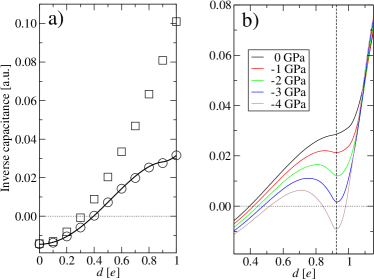
Figure 3: Dielectric properties. (a) Calculated inverse capacitance in the free-stress ($\gamma$, circles) and fixed strain ($\gamma^{\eta}$, squares) limits. The points were obtained by extracting the symmetric $6\times 6$ elementary response tensors by finite differences (steps of $\pm$0.001 were taken for each parameter) for each value of $d$; the continuous curve is the result of numerical differentiation of the splined potential. (b) Evolution of $\gamma$ for increasingly larger negative pressures.

Having verified the accuracy and consistency of our method, we now demonstrate its utility by analyzing the second derivative of the internal energy (or equivalently the first derivative of the potential) as a function of $d$, which corresponds to the inverse capacitance $\gamma$. The symbols in Fig. 3(a) show the linear-response values of both $\gamma^{\eta}$ and $\gamma$, which are identical in the non-piezoelectric cubic limit. The numerical derivative of the splined potential of Fig. 2(a) accurately matches $\gamma$, again confirming the high numerical quality of our calculations. Fig. 3(a) shows that the inverse capacitance is negative for $0<d<0.395$ [the zero-crossing point corresponds to the inflection point of the $U(d)$ curve of Fig. 2(b), and to the minimum of $\bar{\varepsilon}(d)$ of Fig. 2(a)]. This is indicative of the fact that cubic PbTiO₃ is characterized by a ferroelectric instability, which means that the $U(d)$ curve has a negative curvature around the saddle point $d=0$. We suggest, therefore, that the constrained-$\mathbf{D}$ inverse capacitance at $d=0$, while not accessible experimentally (since it corresponds to an unstable configuration of the crystal), is a useful indicator of the strength of the ferroelectric instability. As such, it can play an important role in determining the critical thickness for ferroelectricity in thin perovskite films; in particular, a material with lower $\gamma$ should be ferroelectric down to smaller thicknesses, provided that the depolarizing effects due to the ferroelectric/electrode interface are equally important Junquera/Ghosez:2003 . Note that in our terminology one ferroelectric can be both stronger and less polar than another if it has a more negative $\gamma$ but a smaller $|P_{s}|$.

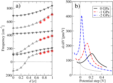
Figure 4: Lattice-dynamical and piezoelectric properties. (a) Longitudinal (filled symbols, continuous curves) and transverse (open symbols, dashed curves) optical modes of $\Gamma_{15}$ symmetry as a function of $d$ at zero pressure. Selected TO frequencies for $\pi$=-4 GPa are shown as red star symbols. (b) Calculated piezoelectric coefficient as a function of external pressure $\pi$ and bias $V$ (thick curves). Results of the Landau-Devonshire model of Refs. haun_pbtio3, and chen_piezo:2003, are shown as a thin dashed curve for comparison.

Piezoelectricity. Interestingly, the free-stress $\gamma(D)$ curve in Fig. 3(a) shows a peculiar plateau for $0.8<d<1.0$, indicative of a “softening” of the response of the crystal to the applied electric field. This behavior is surprising, as an electric field of increasing strength would rather be expected to drive a perovskite crystal further into the anharmonic regime, with a consequent progressive hardening of the overall dielectric response chen_piezo:2003 . To analyze this effect, we start by observing that the evolution of the fixed-strain $\gamma^{\eta}$ dielectric response as a function of $d$ is essentially featureless. This indicates that optical phonons alone cannot be responsible for the effect, and volume (and/or cell-shape) relaxations are crucially involved. To investigate the coupling between the volume and the dielectric response, we repeated our calculations within a negative hydrostatic pressure by using the mixed fixed-$D$, fixed-$\pi$ enthalpy defined in Eq. (10). The results for the free-stress $\gamma(D)$, plotted in Fig. 3 (b), show a dramatic influence of the external pressure on the dielectric response of the system. In particular, the plateau in $\gamma(D)$ becomes an increasingly deeper local minimum, which crosses the $\gamma=0$ axis for $\pi$ between $-$3 and $-$4 GPa; the local minimum is approximately centered in $d=0.925$ for all values of $\pi$.

A negative $\gamma$ indicates a structural instability, and structural instabilities in ferroelectric systems are usually understood in terms of “soft” phonon modes. In order to see whether this picture applies here, we plotted in Fig. 4(a) the zone-center polar mode frequencies as a function of $d$. At zero pressure, the curves show no notable irregularity, consistent with the smooth evolution of the fixed-strain response $\gamma^{\eta}$. Remarkably, the external pressure has a negligible influence on such frequencies, which remain practically unchanged for the strained crystal at the same value of $d$, confirming our hypothesis that the effect is essentially of piezoelectric nature.

Pursuing this idea, we combined the values of the potential drop $V(d)$ with the equilibrium values of out-of-plane lattice parameter, and calculated the free-stress piezoelectric coefficient by numerical differentiation as

$$h=-\frac{dc}{dV}\,.$$ (20)

The results, plotted in Fig. 4(b), show for zero pressure a clear peak at $V\sim 0.2V$, corresponding to a value of the internal field of about 450 MV/m. We identify this peak with the plateau in the inverse capacitance curve of Fig. 3(a). For incresingly large negative pressures, the piezoelectric peak becomes sharper and shifts to smaller values of the potential; for $\pi<-3$ GPa (not shown) the piezoelectric coefficient diverges, corresponding to the crossover to the unstable region in Fig. 3 (b).

These results shed light on the recent experimental measurements of Ref. grigoriev, , where a remarkable anomaly in the piezoelectric response of PZT films in high fields ($\mathcal{E}=200-300$ MV/m) was detected. Such an anomaly was rationalized in terms of a transition to a supertetragonal state, which previous first-principles calculations tinte predicted to be stable in PbTiO₃ under an applied negative hydrostatic pressure. However, the question remained whether the electric field might actually produce such a transition within the experimental range of applied fields. Our results demonstrate that the piezoelectric coupling is indeed capable of driving such a transition, at least under isotropic free-stress boundary conditions. (In future work, we plan to extend these investigations by considering epitaxial strain clamping effects.) We note that our calculated value of the piezoelectric coefficient of PbTiO₃ at zero field and pressure ($h=82.5$ pm/V) is in excellent agreement with previous Landau-Devonshire theories haun_pbtio3 ; chen_piezo:2003 , but the evolution of $h$ for nonzero values of the applied potential substantially differs [see Fig. 4 (b)]. For small values of the electric field, in particular, our ab-initio results indicate that $h$ remains roughly constant. Then $h$ increases significantly at higher fields, up to a value $\mathcal{E}\sim$ 450 MV/m, where it starts decreasing again. A monotonic decrease was predicted instead by the model of Ref. chen_piezo:2003, . This result, therefore, has important implications for the tunability of the piezoresponse of lead titanate crystals.

Summary and outlook. In conclusion, we have presented a formalism that provides full control over the electrical degrees of freedom in a periodic first-principles electronic-structure calculation. We have in mind several immediate applications for our method. First and foremost, fixing $D$ in ferroelectric capacitors by using the methods of Ref. Stengel/Spaldin:2007, will allow for a detailed analysis of the microscopic mechanisms determining the depolarizing field, both in the linear and anharmonic regime, an issue which is central to the development of efficient ferroelectric devices. Second, imposing constant-$D$ electrical boundary conditions has the virtue of making the force-constant matrix of layered heterostructures short-ranged in real space. This allows one to accurately model the polarization and response of complex superlattices, capacitors and interfaces in terms of the electrical properties of the elementary building blocks; a demonstration of this strategy was recently reported in Ref. xifan_2008, . Third, complex couplings between different order parameters can now be treated with unprecedented flexibility, opening new avenues in the theoretical study of magnetoelectric multiferroics and improper ferroelectrics.

Acknowledgements. This work was supported by the Department of Energy SciDac program on Quantum Simulations of Materials and Nanostructures, grant number DE-FC02-06ER25794 (M.S. and N.A.S.), and by ONR grant N00014-05-1-0054 (D.V.).

References

- (1) King-Smith, R. D. & Vanderbilt, D. Theory of polarization of crystalline solids. Phys. Rev. B 47, R1651–R1654 (1993).
- (2) Souza, I., Íñiguez, J. & Vanderbilt, D. First-principles approach to insulators in finite electric fields. Phys. Rev. Lett. 89, 117602 (2002).
- (3) Umari, P. & Pasquarello, A. Ab initio molecular dynamics in a finite homogeneous electric field. Phys. Rev. Lett. 89, 157602 (2002).
- (4) Diéguez, O. & Vanderbilt, D. First-principles calculations for insulators at constant polarization. Phys. Rev. Lett. 96, 056401 (2006).
- (5) Vanderbilt, D. Soft self-consistent pseudopotentials in a generalized eigenvalue formalism. Phys. Rev. B 7892 (1990).
- (6) Blöchl, P. E. Projector augented-wave method. Phys. Rev. B 50, 17953–17979 (1994).
- (7) Vanderbilt, D. Berry-phase theory of proper piezoelectric response. J. Phys. Chem. Solids 61, 147–151 (2000).
- (8) Wu, X., Vanderbilt, D. & Hamann, D. R. Systematic treatment of displacements, strains, and electric fields in density-functional perturbation theory. Phys. Rev. B 72, 035105 (2005).
- (9) Baroni, S., de Gironcoli, S. & Corso, A. D. Phonons and related crystal properties from density-functional perturbation theory. Rev. Mod. Phys. 73, 515 (2001).
- (10) Perdew, J. P. & Wang, Y. Accurate and simple analytic representation of the electron-gas correlation energy. Phys. Rev. B 45, 13244 (1992).
- (11) Troullier, N. & Martins, J. L. Efficient pseudopotentials for plane-wave calculations. Phys. Rev. B 43, 1993–2006 (1991).
- (12) Monkhorst, H. J. & Pack, J. D. Special points for brillouin-zone integrations. Phys. Rev. B 13, 5188–5192 (1976).
- (13) Stengel, M. & Spaldin, N. A. Ab-initio theory of metal-insulator interfaces in a finite electric field. Phys. Rev. B 75, 205121 (2007).
- (14) Stengel, M. & Spaldin, N. A. Accurate polarization within a unified Wannier function formalism. Phys. Rev. B 73, 075121 (2006).
- (15) Junquera, J. & Ghosez, P. Critical thickness for ferroelectricity in perovskite ultrathin films. Nature 422, 506–509 (2003).
- (16) Haun, M. J., Furman, E., Jang, S. J., McKinstry, H. A. & Cross, L. E. Thermodynamic theory of PbTiO3. J. Appl. Phys. 62, 3331–3338 (1987).
- (17) Chen, L., Nagarajan, V., Ramesh, R. & Roytburd, A. L. Nonlinear electric field dependence of piezoresponse in epitaxial ferroelectric lead zirconate titanate thin films. J. Appl. Phys. 94, 5147–5152 (2003).
- (18) Grigoriev, A. et al. Nonlinear piezoelectricity in epitaxial ferroelectrics at high electric fields. Phys. Rev. Lett. 100, 027604 (2008).
- (19) Tinte, S., Rabe, K. M. & Vanderbilt, D. Anomalous enhancement of tetragonality in PbTiO3 induced by negative pressure. Phys. Rev. B 68, 144105 (2003).
- (20) Wu, X., Stengel, M., Rabe, K. M. & Vanderbilt, D. Predicting polarization and nonlinear dielectric response of arbitrary perovskite superlattice sequences. Phys. Rev. Lett. 101, 087601 (2008).