Cascades, thermalization and eddy viscosity in helical Galerkin truncated Euler flows

Abstract

The dynamics of the truncated Euler equations with helical initial conditions are studied. Transient energy and helicity cascades leading to Kraichnan helical absolute equilibrium at small scales are obtained for the first time. The results of [Cichowlas et al. Phys. Rev. Lett. 95, 264502 (2005)] are extended to helical flows. Similarities between the turbulent transient evolution of the ideal (time-reversible) system and viscous helical flows are found. The observed differences in the behavior of truncated Euler and (constant viscosity) Navier-Stokes are qualitatively understood using the concept of eddy viscosity. The large scales of truncated Euler equations are then shown to follow quantitatively an effective Navier-Stokes dynamics based on a variable (scale dependent) eddy viscosity.

The role played by helicity in turbulent flows is not completely understood. Helicity is relevant in many atmospheric processes, such as rotating convective (supercell) thunderstorms, the predictability of which may be enhanced because of its presence heli . However helicity, which is a conserved quantity in the three dimensional Euler equation, plays no role in the original theory of turbulence of Kolmogorov. Later studies of absolute equilibrium ensembles for truncated helical Euler flows by Kraichnan KRA73 gave support to an scenario where in helical turbulent flows both the energy and the helicity cascade towards small scales Helcas-BFLLM , a phenomena recently verified in numerical simulations BorueOrszag97 ; Eyink03 ; MininniPouquet06 . The thermalization dynamics of the non-helical spectrally truncated Euler flows were studied in CBDB-echel . However, Kraichnan helical equilibrium solutions were never directly observed in simulations. Note that the Galerkin truncated non-helical Euler dynamics was recently found to emerge as the asymptotic limit of high order hyperviscous hydrodynamics and that bottlenecks observed in viscous turbulence may be interpreted as an incomplete thermalization frisch-2008 .

In this letter we study truncated helical Euler flows, and consider the transient turbulent behavior as well as the late time equilibrium of the system. Here is a short summary of our main results. The relaxation toward a Kraichnan helical absolute equilibrium KRA73 is observed for the first time. Transient mixed energy and helicity cascades are found to take place while more and more modes gather into the Kraichnan time-dependent statistical equilibrium. It was shown in CBDB-echel that, due to the effect of thermalized small-scales, the spectrally truncated Euler equation has long-lasting transients behaving similarly to the dissipative Navier-Stokes equation. These results, obtained for non-helical flows, are extended to the helical case. The concept of eddy viscosity, as previously developed in CBDB-echel and GKMEB2fluid , is used to qualitatively explain differences observed between truncated Euler and high-Reynolds number (fixed viscosity) Navier-Stokes. Finally, the truncated Euler large scale modes are shown to quantitatively follow an effective Navier-Stokes dynamics based on a (time and wavenumber dependent) eddy viscosity that does not depend explicitly on the helicity content in the flow.

Performing spherical Galerkin truncation at wave-number $k_{\rm max}$ on the incompressible ($\nabla\cdot{\bf u}=0$) and spatially periodic Euler equation ${\partial_{t}{\bf u}}+({\bf u}\cdot\nabla){\bf u}=-\nabla p$ yields the following finite system of ordinary differential equations for the Fourier transform of the velocity ${\bf\hat{u}}({\bf k})$ (${\bf k}$ is a 3 D vector of relative integers satisfying $|{\bf k}|\leq k_{\rm max}$):

$${\partial_{t}{\hat{u}}_{\alpha}({\bf k},t)}=-\frac{i}{2}{\mathcal{P}}_{\alpha\beta\gamma}({\bf k})\sum_{\bf p}{\hat{u}}_{\beta}({\bf p},t){\hat{u}}_{\gamma}({\bf k-p},t),$$ (1)

where ${\mathcal{P}}_{\alpha\beta\gamma}=k_{\beta}P_{\alpha\gamma}+k_{\gamma}P_{\alpha\beta}$ with $P_{\alpha\beta}=\delta_{\alpha\beta}-k_{\alpha}k_{\beta}/k^{2}$.

This time-reversible system exactly conserves the energy $E=\sum_{k}E(k,t)$ and helicity $H=\sum_{k}H(k,t)$, where the energy and helicity spectra $E(k,t)$ and $H(k,t)$ are defined by averaging respectively ${\frac{1}{2}}|{\bf\hat{u}}({\bf k^{\prime}},t)|^{2}\,$ and ${\bf\hat{u}}({\bf k^{\prime}},t)\cdot{\bf\hat{\omega}}({\bf-k^{\prime}},t)$ (${\bf\omega=\nabla\times{\bf u}}$ is the vorticity) on spherical shells of width $\Delta k=1$. It is trivial to show from the definition of vorticity that $|H(k,t)|\leq 2kE(k,t)$.

We will use as initial condition ${\bf u}_{0}$ the sum of two ABC (Arnold, Beltrami and Childress) flows in the modes $k=3$ and $k=4$,

$${\bf u}_{0}(x,y,z)={\bf u}_{\rm ABC}^{(3)}(x,y,z)+{\bf u}_{\rm ABC}^{(4)}(x,y,z)$$ (2)

where the basic ABC flow is a maximal helicity stationary solution of Euler equations in which the vorticity is parallel to the velocity, explicitly given by

$${\bf u}_{\rm ABC}^{(k)}(x,y,z) = \frac{u_{0}}{k^{2}}\left\{\left[B\cos(ky)+C\sin(kz)\right]\hat{x}+\right.{}$$ (3)

$${}+\left[A\sin(kx)+C\cos(kz)\right]\hat{y}+{}$$

$${}+\left.\left[A\cos(kx)+B\sin(ky)\right]\hat{z}\right\}.$$

The parameters will be set to $A=0.9$, $B=1$, $C=1.1$ and $u_{0}=(A^{2}+B^{2}+C^{2})^{-1/2}(1/3^{4}+1/4^{4})^{-1/2}$. With this choice of normalization the initial energy is $E=0.5$ and helicity $H=3\times 4\times(3^{3}+4^{3})/(3^{4}+4^{4})=3.24$.

Numerical solutions of equation (1) are efficiently produced using a pseudo-spectral general-periodic code PabloCode1 with $512^{3}$ Fourier modes that is dealiased using the $2/3$ rule Got-Ors by spherical Galerkin truncation at $\textbf{k}_{\rm max}=170$. The equations are evolved in time using a second order Runge-Kutta method, and the code is fully parallelized with the message passing interface (MPI) library. The numerical method used is non-dispersive and conserves energy and helicity with high accuracy.

Fig.1 shows the time-evolution of the energy and helicity spectra that evolve from (2) compensated by $k^{5/3}$.

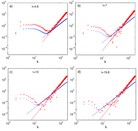
Figure 1: Compensated energy ($\bullet\bullet\bullet$) and helicity spectra ($\times\times\times$) with the predictions (4) in solid lines and (6) in dotted lines. a) $t=4.8$. b) $t=7$. c) $t=10$. d) $t=19.8$.

The plots clearly display a progressive thermalization similar to that obtained in Cichowlas et al.CBDB-echel but with the non zero helicity cascading to the right.

The truncated Euler equation dynamics is expected to reach at large times an absolute equilibrium that is a statistically stationary gaussian exact solution of the associated Liouville equation OrszagAnalytTheo . When the flow has a non vanishing helicity, the absolute equilibria of the kinetic energy and helicity predicted by Kraichnan KRA73 are

$$E(k)=\frac{k^{2}}{\alpha}\frac{4\pi}{1-\beta^{2}k^{2}/\alpha^{2}}\,;\hskip 2.84544ptH(k)=\frac{k^{4}\beta}{\alpha^{2}}\frac{8\pi}{1-\beta^{2}k^{2}/\alpha^{2}}$$ (4)

where $\alpha>0$ and $\beta k_{\rm max}<\alpha$ to ensure integrability. The values of $\alpha$ and $\beta$ are uniquely determined by the total amount of energy and helicity (verifying $|H|\leq 2k_{\rm max}E$) contained in the wavenumber range $[1,k_{\rm max}]$ KRA73 .

The final values of $\alpha$ and $\beta$ (when total thermalization is obtained) corresponding to the initial energy and helicity are $\alpha=4.12\times 10^{7}$ and $\beta=7695$. Therefore the dimensionless number $\beta^{2}k^{2}/\alpha^{2}$ is at most of the order $10^{-4}$ and equations (4) thus lead to almost pure power laws for the energy and helicity spectra, as is manifest in Fig1.d. Fig. 1 thus shows for the first time a time evolving helical quasi-equilibrium.

In order to analyze the run in the spirit of Cichowlas et al. CBDB-echel we define $k_{\rm th}(t)$ as the wavenumber where the thermalized power-law zone starts. We define the thermalized energy and helicity as

$${E}_{\rm th}(t)=\sum_{k_{\rm th}(t)}^{k_{\rm max}}E(k,t)\,;\hskip 8.5359pt{H}_{\rm th}(t)=\sum_{k_{\rm th}(t)}^{k_{\rm max}}H(k,t)$$ (5)

where $E(k,t)$ and $H(t,k)$ are the energy and helicity spectra.

The temporal evolutions of $E_{\rm th},H_{\rm th}$ and $k_{\rm th}(t)$ are shown in Fig. 2.

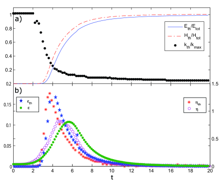
Figure 2: a) Temporal evolution of $E_{\rm th}$ ($-$) ,$H_{\rm th}$ ($\cdot-\cdot$) and $k_{\rm th}(t)$ ($\cdots$) normalized by their respective initial values. $E_{\rm tot}=0.5$, $H_{\rm tot}=3.24$ and $k_{\rm max}=170$. b) Left vertical axis: temporal evolution of $\epsilon_{\rm th}=\frac{dE_{\rm th}}{dt}$ ($\bigstar\bigstar\bigstar$) and Navier-Stokes energy dissipation $\epsilon=2\nu_{0}\sum_{k=1}^{k_{\rm max}}k^{2}E(k)$ ($\bullet\bullet\bullet$). Right vertical axis: $\eta_{\rm th}=\frac{dH_{\rm th}}{dt}$ ($***$) and NS helicity dissipation $\eta=\nu_{0}\sum_{k=1}^{k_{\rm max}}k^{2}H(k)$ ($\circ\circ\circ$).

The values of $\alpha(t)$ and $\beta(t)$ during thermalization can then be obtained from $E_{\rm th}(t),H_{\rm th}(t)$ and $k_{\rm th}(t)$ by inverting the system of equations (5) using $\frac{\beta^{2}}{\alpha^{2}}k_{\rm max}^{2}\ll 1$.

The Kraichnan prediction (4) for the high-$k$ part of the spectra are shown (in solid lines) in Fig. 1. The plot shows an excellent agreement with the prediction.

The low-$k$ part of the compensated spectrum presents a flat zone that amounts to $k^{-5/3}$ scaling for both the energy and helicity spectra. This $k^{-5/3}$ behavior was predicted by Brissaud et al. Helcas-BFLLM in viscous fluids when there are simultaneous energy and helicity cascades. The energy and helicity fluxes, $\epsilon$ and $\eta$ respectively, determine the prefactor in the inertial range of the spectra:

$$E(k)\sim\epsilon^{2/3}k^{-5/3},\hskip 14.22636ptH(k)\sim\eta\epsilon^{-1/3}k^{-5/3},$$ (6)

Helical flows have been also studied in high Reynolds number numerical simulations of the Navier-Stokes (NS) equation. Simultaneous energy and helicity cascades leading to the scaling (6) have been confirmed when the system is forced at large scales BorueOrszag97 ; Eyink03 ; MininniPouquet06 .

The energy and helicity fluxes $\epsilon$ and $\eta$ at intermediate scales in our truncated Euler simulation can be estimated using the time derivative of the thermalized energy and helicity: $\epsilon_{\rm th}=\frac{dE_{\rm th}}{dt}$ and $\eta_{\rm th}=\frac{dH_{\rm th}}{dt}$, whose temporal evolutions are shown in Fig. 2. The predictions (6) for the low-$k$ part of the spectra are shown (in dotted lines) in Fig. 1. The plot shows a good agreement with the data. Note that Fig. 1.a corresponds to $t=4.8$, that is just after the time when both the maximum energy and helicity fluxes (to be interpreted below as “dissipation” rates of the non-thermalized components of the energy and the helicity) are achieved, see Fig. 2. In this way $E_{\rm th}$ and $H_{\rm th}$ determine the thermalized part of the spectra while their time derivative determines an inertial range.

We now compare the dynamics of the truncated Euler equation with that of the unforced high-Reynolds number NS equation (i.e. Eq.(1) with $-\nu_{0}k^{2}{\hat{u}}_{\alpha}({\bf k},t)$ added in the r.h.s.) using the initial condition (2). The viscosity is set to $\nu_{0}=5\times 10^{-4}$, the smallest value compatible with accurate computations using $k_{\rm max}=170$. A behavior qualitatively similar to that of the truncated Euler equation is obtained (see Fig. 2b). However, the maxima of the energy and helicity fluxes (or dissipation rates) occur later, and with smaller values.

We refered above to “dissipation” in the context of the ideal (time-reversible) flow. A proper definition of dissipation in the truncated Euler flow is now in order. Thermalized modes in truncated Euler are known to provide an eddy viscosity $\nu_{\rm{eddy}}$ to the modes with wavenumbers below the transition wavenumber CBDB-echel . It was shown in GKMEB2fluid that Monte-Carlo determinations of $\nu_{\rm eddy}$ are given with good accuracy by the Eddy Damped Quasi-Normal Markovian (EDQNM) two-point closure, previously known to reproduce well direct numerical simulation results BosBertoglioEDQNM . For helical flows, the EDQNM theory provides coupled equations for the energy and helicity spectra EDQNM-Andre-Lesieur , in which using (4) in an analogous way to GKMEB2fluid we find a very small correction of $\nu_{\rm{eddy}}$ that depends on the total amount of helicity and is of order $\Delta\nu_{\rm{eddy}}/\nu_{\rm{eddy}}\sim\beta k_{\rm max}/\alpha\sim 10^{-2}$. Thus the presence of helicity does not affect significantly the dissipation at large scales and can be safely neglected in the eddy viscosity expressions. This eddy viscosity has a strong dependence in $k$ and can also be obtained, in the limit $k/k_{\rm max}\rightarrow 0$, from the EDQNM eddy viscosity of Lesieur and Schertzer LesieruSchertezerEDQNMExpa using here an energy spectrum $E(k)\sim k^{2}$. The result reads

$$\nu_{\rm{eddy}}=\frac{\sqrt{E_{\rm{th}}}}{k_{\rm{max}}}\frac{7}{\sqrt{15}\lambda},$$ (7)

with $\lambda=0.36$. The eddy viscosity $\nu_{\rm{eddy}}$ is thus an increasing function of time, see $E_{\rm{th}}(t)$ in Fig. 2.

The time-evolution of truncated Euler and Navier-Stokes spectra are compared in Fig. 3. At early times the value of $E_{\rm{th}}$ is very small and therefore the NS viscosity $\nu_{0}$ is larger than $\nu_{\rm{eddy}}$, as manifested by the NS dissipative zone in Fig. 3.a. As $E_{\rm{th}}(t)$ increases, both viscosities became equal ($t=2.7$). Later, at $t=3.8$, the Navier-Stokes spectrum crosses the truncated Euler one (Fig. 3b). The eddy viscosity $\nu_{\rm{eddy}}$ is then much larger than $\nu_{0}$ and the truncated Euler dissipative zone lies below the NS one, see Fig. 3c. This behavior is also conspicuous when the spectra are compared at maximum energy-dissipation time ($t=4.4$ for truncated Euler and $t=5.6$ for NS), see Fig. 3d.

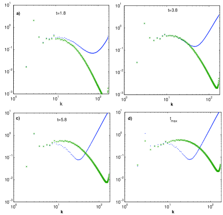
Figure 3: Compensated energy spectra of truncated Euler ($\cdots$) and Navier-Stokes ($\times\times\times$). a) $t=1.8$, b) $t=3.8$, c) $t=5.8$. d) Maximum energy-dissipation time ($t=4.4$ for truncated Euler and $t=5.6$ for NS).

The variation in time of $\nu_{\rm{eddy}}$ thus explains qualitatively the different behavior of the truncated Euler and Navier-Stokes spectra in Fig. 3. We now proceed to check more quantitatively the validity of an effective dissipation description of thermalization in truncated Euler. To wit, we introduce an effective Navier-Stokes equation for which the dissipation is produced by an effective viscosity that depends on time and wavenumber.

We will use the effective viscosity obtained in GKMEB2fluid which is consistent with both direct Monte-Carlo calculations and EDQNM closure and is explicitly given by

$$\nu_{\rm{eff}}(k)=\nu_{\rm{eddy}}e^{-3.97k/k_{\rm{max}}},$$

with $\nu_{\rm{eddy}}$ given in Eq. (7).

We thus integrate Eq. (1) with the viscous term $-\nu_{\rm{eff}}(k)k^{2}{\hat{u}}_{\alpha}({\bf k},t)$ added in the right hand side. The parameter $E_{\rm{th}}$ that fixes the eddy viscosity in Eq. (7) is evolved using the effective NS dissipation by

$$\frac{dE_{\rm{th}}}{dt}=\sum_{k=1}^{k_{\rm max}}2\nu_{\rm{eff}}(k)k^{2}E(k).$$ (8)

This ensures consistency between the effective NS dissipated energy and the truncated Euler thermalized energy that drives $\nu_{\rm{eddy}}$.

To initialize the effective NS equation we integrate the truncated Euler equation (1) with the initial condition (2) until the $k^{2}$-thermalized zone is clearly present ($t=4.77$). The value of $E_{\rm{th}}$ is then computed using equations (5). The low-passed velocity ${\bf u}^{<}$, defined by

$${\bf u}^{<}(\textbf{r})=\sum\frac{1}{2}\left(1+\tanh{\left[2({|\textbf{k}|-k_{\rm th}})\right]}\right)\hat{{\bf u}}_{\textbf{k}}e^{i\textbf{k}\cdot\textbf{r}}$$

is used as initial data for the effective Navier-Stokes dynamics.

Results of a truncated Euler and effective NS with $k_{\rm max}=85$ are shown in Fig. 4. In Fig. 4.a the energy and helicity dissipated in effective NS [$E_{\rm tot}-E(t)$ and $H_{\rm tot}-H(t)$ respectively] are compared to $E_{\rm th}$ and $H_{\rm th}$ showing a good agreement. Next, the temporal evolution of both energy spectra from the initial time $t=5.3$ (Fig. 4.b) to $t=20$ (Fig. 4.e) is confronted, demonstrating that the low-$k$ dynamics of truncated Euler is well reproduce by the effective Navier-Stokes equations.

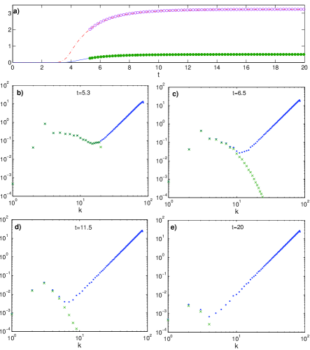
Figure 4: Effective NS run with $k_{\rm max}=85$. a) Temporal evolution of $E_{\rm th}$ ($-$), $H_{\rm th}$ ($\cdot-\cdot$) from truncated Euler, energy ($\bullet\bullet\bullet$) and helicity ($\circ\circ\circ$) from effective NS. b-e) Temporal evolution of compensated energy spectra of truncated Euler ($\cdots$) and effective Navier-Stokes ($\times\times\times$) .

In summary, we observed the relaxation of the truncated Euler dynamics toward a Kraichnan helical absolute equilibrium. Transient mixed energy and helicity cascades were found to take place. Eddy viscosity was found to qualitatively explain the different behaviors of truncated Euler and (constant viscosity) Navier-Stokes. The large scale of Galerkin truncated Euler were shown to quantitatively follow an effective Navier-Stokes dynamics based on a variable helicity-independent eddy viscosity. In conclusion, with its built-in eddy viscosity, the Galerkin truncated Euler equations appears as a minimal model of turbulence.

Acknowledgments: We acknowledge discussions with U. Frisch. and J.Z. Zhu. P.D.M. is a member of the Carrera del Investigador Científico of CONICET. The computations were carried out at NCAR and IDRIS (CNRS).

References

- [1] D.K. Lilly. J. Atmosph. Sc., 43:126–140, 1986.
- [2] R.H. Kraichnan. J. Fluid Mech., 59:745–752, 1973.
- [3] A. Brissaud, U. Frisch, J. Leorat, M. Lesieur, and A. Mazure. Physics Of Fluids, 16(8):1366–1367, 1973.
- [4] V. Borue and S.A. Orszag. Physical Review E, 55(6, Part A):7005–7009, JUN 1997.
- [5] Q.N. Chen, S.Y. Chen, and G.L. Eyink. Physics of Fluids, 15(2):361–374, FEB 2003.
- [6] P. D. Mininni, A. Alexakis, and A. Pouquet. Physical Review E, 74(1, Part 2), JUL 2006.
- [7] C. Cichowlas, P. Bonaïti, F. Debbasch, and M.E. Brachet. Phys. Rev. Lett., 95(26), 2005.
- [8] U. Frisch, S. Kurien, R. Pandit, W. Pauls, S.S. Ray, A. Wirth, and J.Z. Zhu. http://arxiv.org/abs/0803.4269, 2008.
- [9] G. Krstulovic and M.E. Brachet. Physica D. doi:10.1016/j.physd.2007.11.008, 2007.
- [10] D.O. Gómez, P.D. Mininni, and P. Dmitruk. Physica Scripta, 2005:123–127, 2005. Advances in Space Research, 35:889–907, 2005.
- [11] D. Gottlieb and S. A. Orszag. SIAM, Philadelphia, 1977.
- [12] S.A. Orszag. J. Fluid Mech., 41(363), 1970.
- [13] W. J. T. Bos and J.-P. Bertoglio. Phys. Fluids, 18(071701), 2006.
- [14] J.C. André and M. Lesieur. J. Fluid Mech., 81:187–207, 1977.
- [15] M. Lesieur and D. Schertzer. J. Mec., 609(17), 1978.