Heat transfer in sunspot penumbrae

Abstract

Context. Observations at 0$\aas@@fstack{\prime\prime}$1 have revealed the existence of dark cores in the bright filaments of sunspot penumbrae. Expectations are high that such dark-cored filaments are the basic building blocks of the penumbra, but their nature remains unknown.

Aims. We investigate the origin of dark cores in penumbral filaments and the surplus brightness of the penumbra. To that end we use an uncombed penumbral model.

Methods. The 2D stationary heat transfer equation is solved in a stratified atmosphere consisting of nearly horizontal magnetic flux tubes embedded in a stronger and more vertical field. The tubes carry an Evershed flow of hot plasma.

Results. This model produces bright filaments with dark cores as a consequence of the higher density of the plasma inside the tubes, which shifts the surface of optical depth unity toward higher (cooler) layers. Our calculations suggest that the surplus brightness of the penumbra is a natural consequence of the Evershed flow, and that magnetic flux tubes about 250 km in diameter can explain the morphology of sunspot penumbrae.

1 Introduction

At high angular resolution, penumbral filaments are observed to consist of a central dark lane and two lateral brightenings (Scharmer et al. 2002; Sütterlin et al. 2004; Rouppe van der Voort et al. 2004; Bellot Rubio et al. 2005; Langhans et al. 2007). The common occurrence of dark-cored filaments and the fact that their various parts show a coherent behavior have raised expectations that they could be the fundamental constituents of the penumbra. Their nature, however, remains enigmatic.

One possibility is that dark-cored filaments represent magnetic flux tubes carrying a hot flow. This would support the uncombed model proposed by Solanki & Montavon (1993), which describes the penumbra as a collection of nearly horizontal flux tubes embedded in a more vertical background field. The uncombed model is, by far, the most successful representation of the fine structure of the penumbra currently available. It explains the polarization profiles of visible and near-infrared lines observed in sunspots (e.g., Beck 2008), including their net circular polarization (NCP). This success is not trivial, since the behavior of the NCP depends on the details of the magnetic and velocity fields in a very subtle way (see Müller et al. 2002; Borrero et al. 2007; Tritschler et al. 2007, and references therein). The uncombed model is supported not only by observations, but also by theoretical work. Schlichenmaeier et al. (1998) and Schlichenmaier (2002) performed numerical simulations of penumbral flux tubes in the thin tube approximation. These calculations show filaments whose morphology and dynamics are very similar to those actually observed in the penumbra (Schlichenmaier 2003). Moreover, the simulations offer a natural explanation for the Evershed flow, the most conspicuous dynamical phenomenon of sunspots. In spite of these achievements, it is still not known whether magnetic flux tubes can also account for the existence of dark cores in penumbral filaments and, more importantly, for the surplus brightness of the penumbra. Schlichenmaier & Solanki (2003) suggested that hot upflows along magnetic flux tubes would indeed be able to heat the penumbra to the required degree if the tubes return to the solar interior after they have released their energy in the photosphere. At that time the existence of opposite-polarity field lines in the penumbra was unclear, but now it is a well-established observational fact: submerging flux tubes have been detected from Stokes inversions and even imaged directly by Hinode (Sainz Dalda & Bellot Rubio 2008). Thus, the Evershed flow remains the best candidate to explain the brightness of the penumbra.

Another possibility is that the dark-cored filaments are the manifestation of field-free gaps that pierce the sunspot magnetic field from below. The concept of a gappy penumbra was proposed by Spruit & Scharmer (2006) and Scharmer & Spruit (2006) as an alternative way to explain the surplus brightness of the penumbra, on the assumption that the Evershed flow is not sufficient. The gaps would sustain normal convection, carrying heat to the solar surface. Radiative transfer calculations need to be performed to show that a penumbra consisting of field-free gaps is able to explain the corpus of spectropolarimetric observations accumulated over the years. In its present form, however, the gappy model is bound to experience substantial difficulties when confronted with the observations (Bellot Rubio 2007).

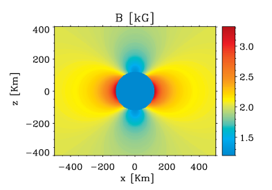
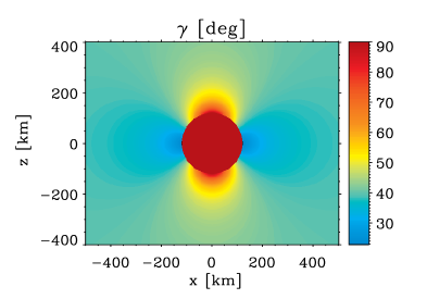
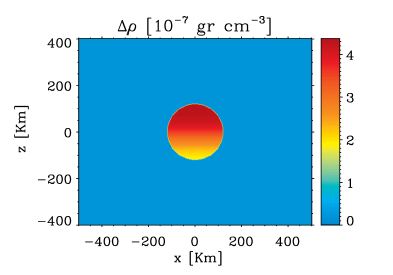
Figure 1: Top left: magnetic field lines in the $xz$-plane. The circle centered at $(0,0)$ km represents the flux tube’s boundary. Note the wrapping of the field lines around the tube. Top right: field strength distribution. Bottom left: field inclination distribution. Bottom right: gas density distribution, for temperatures in the tube and background given by the cool model of Collados et al. (1994). Shown are density differences with respect to the unperturbed atmosphere (Fig. 2).

Recently, Heinemann et al. (2007) have presented first attempts to simulate the penumbra in 3D. The parameters governing the calculations are still far from those of the real sun and, as a consequence, the model sunspot does not show a typical penumbral pattern. Yet, an interesting result of the simulations is the existence of small blobs of plasma with weaker and more inclined fields than their surroundings. The magnetic properties of these structures are reminiscent of those of the flux tubes postulated by the uncombed model. Some of them show a dark lane similar to the dark cores of penumbral filaments. The dark lanes are produced by locally enhanced density and pressure that shift the $\tau=1$ level to higher photospheric layers, where the temperature is lower. This effect was identified for the first time by Schüssler & Vögler (2006) in magnetoconvection simulations of umbral dots. Interestingly, the parameter regime covered by those simulations is not the one relevant to sunspot penumbrae.

Our aim here is to shed some light on the origin of dark-cored penumbral filaments and the surplus brightness of the penumbra. To that end we solve the 2D stationary heat transfer equation in a stratified uncombed penumbra formed by magnetic flux tubes in a stronger background field (Sects. 2 and 3). The tubes carry an Evershed flow of hot plasma. Our calculations show that one such tube would be observed as a dark-cored filament due to the higher density of the plasma within the tube (Sect. 4). We also find that the Everhed flow heats the background atmosphere very efficiently, increasing its temperature. This suggests that the surplus brightness of the penumbra is due to the Evershed flow (Sect. 5.2). Finally, we synthesize polarization maps using the model atmospheres resulting from the simulations and compare them with polarimetric observations of dark-cored filaments (Sect. 5.3).

2 The model

We describe a bright filament in the inner penumbra as a cylindrical flux tube of radius $R$ embedded in a stratified background (umbral) atmosphere. The calculations are performed in a Cartesian coordinate system where the $z$-axis coincides with the vertical and the $y$-direction is defined such that the axis of the tube lies in the $yz$-plane. Since our primary goal is to identify the mechanism(s) responsible for the existence of dark cores, we adopt the simplest magnetic configuration possible, namely a potential field. The field is determined from the conditions $\nabla\cdot\@vec{B}=0$ and $\nabla\times\@vec{B}=0$ in the $xz$-plane, i.e., we neglect variations along the tube axis because they are much smaller than variations perpendicular to it (e.g., Borrero et al. 2004).

In the tube’s interior, the magnetic field is taken to be homogeneous and directed along its axis, which is inclined by an angle $\gamma_{\rm t}$ to the vertical: $\@vec{B}=B_{\rm t}(\sin\gamma_{\rm t}\@vec{e}_{y}+\cos\gamma_{\rm t}\@vec{e}_{z})$. Far from the tube we assume the background magnetic field to be of the form $\@vec{B}=B_{\rm b}(\sin\gamma_{\rm b}\@vec{e}_{y}+\cos\gamma_{\rm b}\@vec{e}_{z}$), so that the field is homogeneous with strength $B_{\rm b}$ and inclination $\gamma_{\rm b}$. We use these conditions, together with the continuity of the radial components at the tube’s boundary, to solve Laplace’s equation in the $xz$-plane. Spectropolarimetry tells us that the field is weaker and more inclined in the tubes (e.g., Bellot Rubio et al. 2004; Borrero et al. 2004), hence we set $B_{\rm t}<B_{\rm b}$ and $\gamma_{\rm t}>\gamma_{\rm b}$. The analytic expressions obtained from the calculations are given in Appendix A.

Figure 1 shows the magnetic configuration of the model with $R=120$ km, $B_{\rm t}=1200$ G, $\gamma_{\rm t}=90^{\circ}$, $B_{\rm b}=2000$ G, and $\gamma_{\rm b}=40^{\circ}$. The background field lines wrap around the tube (top left), leading to enhanced field strengths on either side of the tube and reduced field strengths above and below it (top right). The inclination of the background field also changes depending on the position. In particular, the field above the tube is always more horizontal than $\gamma_{\rm b}$ due to the continuity of the normal components at the tube’s boundary (bottom left).

We require lateral mechanical equilibrium, therefore the total (gas plus magnetic) pressure on both sides of the interface separating the tube from the ambient medium is the same at the same geometrical height $z$. The magnetic field and the temperature then determine the gas density through the ideal gas law (with variable mean molecular weight to account for partial ionization). The equilibrium density distribution shown in the bottom right panel of Fig. 1 corresponds to the case in which the temperatures of the tube and the external medium are those displayed in Fig. 2. As can be seen, a strong density enhancement occurs within the tube to compensate for its lower magnetic pressure.

The condition of lateral force balance does not guarantee vertical equilibrium, so the tube may stretch in the vertical direction. Using simple estimates, however, Borrero et al. (2006) have shown that the vertical stretching could be limited by buoyancy in the subadiabatic layers of the photosphere. Alternatively, non-potential fields may ensure vertical force equilibrium (Borrero 2007). Since there is no generally accepted solution to this problem, we restrict ourselves to the simple magnetic configuration described above in the hope that the results will not depend significantly on the exact topology of the field.

3 Heat transfer equation

To obtain the temperature distribution in the $xz$-plane we consider the stationary ($\partial/\partial t=0$) heat transfer equation

$$\nabla\cdot\@vec{F}=S,$$ (1)

neglecting gradients in the $y$-direction. Here, $\@vec{F}=\@vec{F}_{\rm r}+\@vec{F}_{\rm c}$ represents the heat flux vector and $S$ the various energy sources, including Ohmic dissipation and the Evershed flow. The radiative flux $\@vec{F}_{\rm r}$ is computed using the diffusion approximation

$$\@vec{F}_{\rm r}=-\kappa_{\rm r}\,\nabla T$$ (2)

(e.g., Mihalas 1978), with $\kappa_{\rm r}$ the radiative thermal conductivity and $T$ the temperature. Following Schlichenmaier et al. (1999), we take $\kappa_{\rm r}=16\,D_{\rm F}\,\tilde{\sigma}T^{3}/(k_{\rm R}\rho)$, where $\tilde{\sigma}$ is Stefan-Boltzmann constant, $k_{\rm R}$ the Rosseland mean opacity, $\rho$ the gas density, and $D_{\rm F}$ the flux limiter originally introduced by Levermore & Pomraning (1981). The convective flux $\@vec{F}_{\rm c}$ is evaluated using a linearized mixing length approach (Moreno-Insertis et al. 2002),

$$\@vec{F}_{\rm c}=-\kappa_{\rm c}\,[\nabla T-({\rm d}T/{\rm d}z)_{\rm ad}]\equiv-\kappa_{\rm c}\,\nabla_{\rm c}T,$$ (3)

where $({\rm d}T/{\rm d}z)_{\rm ad}=T({\rm d}P/{\rm d}z)\nabla_{\rm ad}$ represents the adiabatic temperature gradient and $\nabla_{\rm ad}$ the double-logarithmic isentropic temperature gradient. The computation of $\nabla_{\rm ad}$ takes into account the local physical conditions and the partial ionization of hydrogen (Cox & Giuli 1968). In our simulations, $\nabla_{\rm ad}$ varies between 0.1 and 0.4 depending on the layer. The convective transport coefficient $\kappa_{\rm c}$ is evaluated following Spruit (1977). To reduce the efficiency of convection in the presence of magnetic fields we use $T_{\rm eff}=3888$ K, $z_{1}=70$ km, and $k_{0}=0.8\times 10^{-11}$. The calculations are not very sensitive to the details of the energy transport by convection because $\kappa_{\rm c}$ is negligible in photospheric layers. We note, however, that a non-linear treatment of the convective flux, with $\kappa_{\rm c}$ varying with the changing superadiabaticity of the atmosphere, would be more appropriate to deal with large temperature perturbations (Sect. 4.2).

In the absence of penumbral flux tubes, the background atmosphere is a plane-parallel stratified medium where $S=0$ and the physical parameters do not vary with $x$ and $y$. Let us label them with the subscript 0, i.e., $T_{0}(z)$, $\kappa_{\rm r0}(z)$, $\kappa_{\rm c0}(z)$, and so on. Flux tubes embedded in this atmosphere present an obstacle to the heat flow because of their higher gas density, which decreases $\kappa_{\rm r}$. In addition, $S\neq 0$ within the tubes. As a result, the temperature gets modified from $T_{0}(z)$ to $T(x,z)$, but the gas pressure remains the same to ensure horizontal force balance. To find the new equilibrium configuration we solve Eq. (1) iteratively. Let $T_{i}$ be the value of $T(x,z)$ in the $i$-th step. This approximate solution does not satisfy Eq. (1) by an amount

$$\epsilon_{i}\equiv S_{i}-\nabla\cdot[-{\kappa_{\rm r}}_{i}\nabla T_{i}-{\kappa_{\rm c}}_{i}\nabla_{\rm c}T_{i}],$$ (4)

where $S_{i}\equiv S(T_{i})$, ${\kappa_{\rm r}}_{i}\equiv\kappa_{\rm r}(T_{i})$, and ${\kappa_{\rm c}}_{i}\equiv\kappa_{\rm c}(T_{i})$. Our goal is to find a perturbation $\delta T_{i+1}$ such that the new temperature $T_{i+1}\equiv T_{i}+\delta T_{i+1}$ leads to smaller errors, i.e., $\epsilon_{i+1}<\epsilon_{i}$.

Figure 2: Physical parameters in the cool umbral model of Collados et al. (1994). Clockwise from upper left: temperature, gas density, thermal coefficients, and energy fluxes. Radiative and convective parameters are shown in solid and dashed lines, respectively.

In terms of $T_{i+1}$, the heat transfer equation can be written as

$$\nabla\cdot[-{\kappa_{\rm r}}_{i+1}\nabla T_{i+1}-{\kappa_{\rm c}}_{i+1}\nabla_{\rm c}T_{i+1}]=S_{i+1}.$$ (5)

Defining

$${\kappa_{\rm r}}_{i+1}={\kappa_{\rm r}}_{0}+\delta_{0}{\kappa_{\rm r}}_{i+1},$$

$${\kappa_{\rm c}}_{i+1}={\kappa_{\rm c}}_{0}+\delta_{0}{\kappa_{\rm c}}_{i+1},$$ (6)

and neglecting the second-order terms $\delta_{0}{\kappa_{\rm r}}_{i+1}\nabla(\delta T_{i+1})$ and $\delta_{0}{\kappa_{\rm c}}_{i+1}{\nabla}_{\rm c}(\delta T_{i+1})$, Eq. (5) becomes

$$\nabla\cdot[-{\kappa_{\rm r}}_{0}\nabla\delta T_{i+1}-{\kappa_{\rm c}}_{0}\nabla_{\rm c}\delta T_{i+1}]=S_{i+1}-\nabla\cdot[-{\kappa_{\rm r}}_{i+1}\nabla T_{i}-{\kappa_{\rm c}}_{i+1}\nabla_{\rm c}T_{i}].$$ (7)

The heat flux variation due to temperature variations is caused primarily by changes in the temperature gradient, while the effects of changes in the transport coefficients are negligible to first order (Moreno-Insertis et al. 2002). This implies

$${\kappa_{\rm r}}_{0}\nabla\delta T_{i+1} >> [{\kappa_{\rm r}}_{i+1}-{\kappa_{\rm r}}_{i}]\nabla T_{i},$$ (8)

$${\kappa_{\rm c}}_{0}\nabla_{\rm c}\delta T_{i+1} >> [{\kappa_{\rm c}}_{i+1}-{\kappa_{\rm c}}_{i}]\nabla_{\rm c}T_{i},$$ (9)

allowing us to make the approximations ${\kappa_{\rm r}}_{i+1}\simeq{\kappa_{\rm r}}_{i}$ and ${\kappa_{\rm c}}_{i+1}\simeq{\kappa_{\rm c}}_{i}$ in Eq. (7). With the additional assumption that $S_{i+1}\simeq S_{i}$, Eq. (7) can finally be rewritten as

$$\nabla\cdot[-{\kappa_{\rm r}}_{0}\nabla\delta T_{i+1}-{\kappa_{\rm c}}_{0}\nabla_{\rm c}\delta T_{i+1}]=\epsilon_{i},$$ (10)

where the coefficients on the left-hand side depend only on $z$. We seek for periodic solutions of Eq. (10) in the $x$-direction. Thus, the following Neumann boundary conditions are imposed:

$$\delta T_{i}(x,z=z_{\rm min})=0 \forall x,$$ (11)

$$\dot{\delta T}_{i}(x=0,z)=\dot{\delta T}_{i}(x=x_{\rm max},z)=0 \forall z,$$ (12)

where the dots represent derivation with respect to $x$. The first condition prescribes zero temperature variations at the bottom of the computational domain, while the second forces the temperature perturbations to be minimum at the lateral boundaries. With these ingredients, Eq. (10) is solved numerically for each height $z$ using Fourier cosine transforms in the $x$-direction. Convergence ($\mbox{max}\,|{\epsilon_{i}/S_{i}}|<10^{-4}$) is achieved in 5 to 10 iterations.

3.1 Simulation setup

The computational domain is a cube extending 1000 km in the $x$-direction, 3100 km in the $y$-direction, and 1200 km in the $z$-direction. Initially, the cube is filled with an unperturbed umbral atmosphere (the cool model of Collados et al. 1994) with field strength $B_{\rm b}=2000$ G and inclination $\gamma_{\rm b}=40^{\circ}$. Figure 2 shows the run with depth of the temperature, gas density, and radiative and convective parameters in the unperturbed model. A magnetic flux tube is inserted in this atmosphere. It has a radius $R=120$ km, a current sheet 2 km thick, a field strength $B_{\rm t}=1200$ G, and field inclinations varying between 45^∘ and 87^∘ as indicated in Fig. 3. The axis of the tube is placed at a height determined by the field inclination and the distance along the tube, starting with $z=-326$ km at $y=0$ km.

The heat transfer equation is solved in 17 $xz$-planes at different $y$-values (Fig. 3). Each plane is discretized in $501\times 601$ grid points separated by 2 km.

Figure 3: Cut of the computational domain at $x=0$ km, showing a flux tube 120 km in radius. The vertical dotted lines mark the position of the 17 $xz$-planes where we solve the stationary heat transfer equation. The vertical solid line at $y=2083$ km indicates the position of the $xz$-cut displayed in Figs. 4 and 5.

4 Results

We first consider Ohmic dissipation as the only source of energy (Sect. 4.1). Thereafter, we examine how the results are modified by a hot Evershed flow along the magnetic flux tube (Sect. 4.2).

4.1 Ohmic dissipation as the only source of energy

In this case, the source term of the heat transfer equation reduces to $S=j^{2}/\sigma$, where $j$ is the electric current associated with the jump of $\@vec{B}$ at the tube’s boundary (Eq. A) and $\sigma$ the electric conductivity, computed following Kopecký & Kuklin (1969).

Figure 4 shows the simulation results at $y=2083$ km. The tube blocks the energy coming from below and this produces a strong heating of its lower half and the adjacent medium. The associated temperature enhancements, however, are difficult to detect because they occur below the photosphere for the most part.

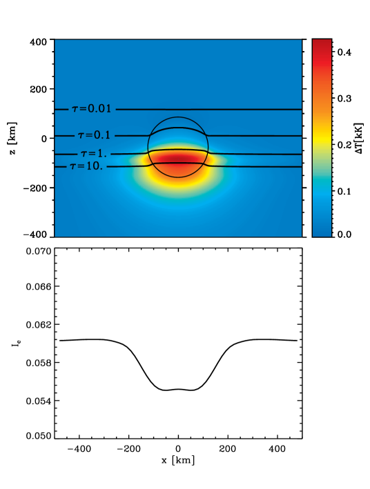
Figure 4: Top: temperature perturbations $\Delta T\equiv T(x,z)-T_{0}(z)$ in the $xz$-plane at $y=2083$ km. Ohmic dissipation is the only energy source considered. The circle represents the flux tube. Solid lines are lines of constant Rosseland optical depth. Bottom: continuum intensity at 487.8 nm emerging from the $y=2083$ km plane, convolved with the Airy point-spread function of a 1-m telescope. The values are normalized to the quiet Sun continuum intensity $I_{\rm QS}$.

The continuum intensity observed at the surface is determined mainly by the temperature prevailing at Rosseland optical depth unity, $\tau_{\rm R}=1$. In the top panel of Fig. 4, lines of constant optical depth are indicated. As can be seen, the $\tau_{\rm R}=1$ level is shifted upwards within the flux tube. The reason is the larger gas density in the tube compared with the external medium, which results from its weaker field strength and the condition of horizontal mechanical equilibrium. The enhanced density increases the opacity and moves the $\tau_{\rm R}=1$ level to higher layers, where the temperature is lower owing to the stratification of the model. In accordance with the Eddington-Barbier relation, the continuum intensity decreases at the position of the tube.

The bottom panel of Fig. 4 shows the continuum intensity emerging from the model at 487.8 nm, as computed by solving the radiative transfer equation and convolving the result with the theoretical Airy point-spread function of a 1-m telescope. The flux tube is darker than its surroundings and do not exhibit bright edges, in clear contradiction with the observations. To reproduce the properties of dark-cored filaments, the walls of the tube should be hotter than the background atmosphere. The $\tau_{\rm R}=1$ level would then encounter higher temperatures at the tube’s boundary, generating two lateral brightenings. Ohmic dissipation in the current sheet, however, cannot provide the necessary heating because of the high conductivity of the plasma. In fact, one would have to reduce the conductivity by at least two orders of magnitude, or to consider extremely thin current sheets (a few meters thick), to heat the walls of the tube to the required degree. Even in that case the dark core would still show smaller continuum intensities than the surroundings. It is therefore necessary to heat not only the walls of the tube, but also the tube itself. In this context, the Evershed flow represents a natural source of energy.

4.2 Heating by the Evershed flow

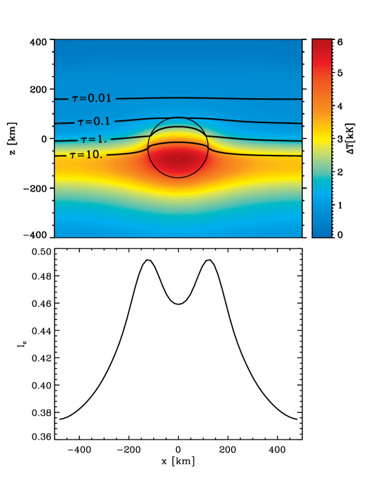
Figure 5: Same as Fig. 4, for the case in which the sources of energy are Ohmic dissipation and a hot Evershed flow.

The Evershed flow is a radial outflow of mass associated with the more inclined magnetic fields of the penumbra (Title et al. 1993; Stanchfield et al. 1997; Schlichenmaier & Schmidt 2000; Westendorp Plaza et al. 2001; Borrero et al. 2005; Bellot Rubio et al. 2006; Rimmele & Marino 2006; Ichimoto et al. 2007).

An Evershed flow of hot plasma along a magnetic flux tube produces an energy flux $\@vec{F}_{\rm E}$ whose divergence can be evaluated from the entropy equation as

$$\nabla\cdot\@vec{F}_{\rm E}=\rho c_{V}\@vec{v}_{\rm E}\,[\nabla T-({\rm d}T/{\rm d}z)_{\rm ad}\@vec{e}_{\rm z}],$$ (13)

where $c_{V}$ is the specific heat at constant volume and $\@vec{v}_{\rm E}$ the flow velocity ($\@vec{v}_{\rm E}=0$ outside the tube). To account for the heating induced by the Evershed flow, we set $S=j^{2}/\sigma+\nabla\cdot\@vec{F}_{\rm E}$ in Eq. (1). We assume that the flow is parallel to the magnetic field (Bellot Rubio et al. 2004), and that its velocity changes with radial distance as dictated by mass conservation due to the density decrease toward higher layers.

The calculation of Eq. (13) cannot be done in 2D because of the term $\nabla T$. To solve the problem we follow an iterative approach. $\nabla T$ is estimated from the temperatures in the plane $y=y_{j-1}$, $T(x,y_{j-1},z)$, and a guess for the temperatures at $y=y_{j}$, $T_{i}(x,y_{j},z)$. Once $S$ is known, the method described in Sect. 3 can be applied to the $y=y_{j}$ plane. This results in a new temperature distribution $T_{i+1}(x,y_{j},z)$ which is used to update $\nabla T$ for the next iteration. Convergence is reached in 10–50 steps. To initialize the calculations, the temperature distribution in the $y=y_{j}$ plane is taken to be the temperature at $y=y_{\rm j-1}$, plus the temperature difference between the two planes in the non-Evershed case.

The temperature excess induced by the flow at $y=0$ km is prescribed as a boundary condition. This condition determines the overall brightness of the flux tube and its surroundings, so it is relatively well constrained. In our calculations we use a temperature excess of 7500 K within the tube at $y=0$ km, to ensure that its brightness is compatible with the observations. An excess of 7500 K is also compatible with the maximum temperatures of $\sim$13 500 K that hot plasma rising adiabatically from the bottom of the convection zone would show at photospheric levels (Borrero 2007).

The upper panel of Fig. 5 displays the simulation results at $y=2083$ km, assuming a flow velocity of $v_{\rm E}=7$ km s^-1 in the first plane. The equilibrium temperature distribution is characterized by an intense heating of the tube and the surroundings, with temperature enhancements of up to 6000 K. This heating increases the brightness of the external medium and modifies the opacity of the plasma in a way that produces filaments with a dark core and two lateral brightenings (lower panel of Fig. 5).

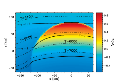
Figure 6: Section of the $xz$-plane at $y=2083$ km showing gas density perturbations $\Delta\rho/\rho_{0}=[\rho(x,z)-\rho_{0}(z)]/\rho_{0}(z)$ induced by the weaker field of the tube and the Evershed flow. Dash-dotted lines represent isotherms. Solid lines indicate lines of constant Rosseland optical depth.

Figure 6 examines in greater detail the origin of these structures. We show the gas density perturbations, $\Delta\rho/\rho_{0}=[\rho(x,z)-\rho_{0}(z)]/\rho_{0}(z)$, in the $xz$-plane at $y=2083$ km together with lines of constant temperature (dash-dotted) and constant Rosseland optical depth (solid). The heating caused by the Evershed flow shifts the $\tau_{R}$ lines to higher layers in and near the tube. For $\tau_{\rm R}\geq 10$, the lines of constant $\tau_{\rm R}$ follow the isotherms closely, i.e., deep in the atmosphere the optical depth scale is primarily determined by the temperature, not by the gas density. This is due to the strong temperature dependence of the H^- opacity. As the tube is approached from $x=-150$ km, the $\tau_{\rm R}=1$ level crosses isotherms corresponding to higher temperatures, which explains the larger continuum intensities of the filament compared with its surroundings. Very close to the tube’s boundary the $\tau_{\rm R}=1$ line encounters regions of even higher temperatures, producing a maximum in the continuum intensity (the lateral brightenings). As soon as the $\tau_{\rm R}=1$ line enters the tube it evolves in a region of enhanced gas density. The increased opacity moves the $\tau_{\rm R}=1$ surface upward by about 40 km, where the temperature is cooler. This generates a dark core.

The density enhancement is more prominent near the top of the tube because the difference of magnetic pressures between the interior and the external medium attains a maximum there with respect to the external gas pressure. The temperature perturbations induced by the Evershed flow decrease the large density contrasts resulting from the weaker field of the tube (bottom right panel of Fig. 1), but this effect is less important in determining the equilibrium density distribution.

Two interesting facts deserve further consideration. First, the $\tau_{\rm R}=0.1$ level is reached at the top of the tube, some 40 km above $\tau_{\rm R}=1$. Thus, a substantial fraction of the line formation region is contained within the flow channel. Second, the density distribution depicted in Fig. 6 tends to stabilize the tube against vertical stretching, since it causes negative buoyancy at the top of the tube. A similar density distribution has been found by Borrero (2007) under the assumption of flux tubes in exact force balance.

Figure 7 displays a continuum (487.8 nm) image of the tube as it would appear through a 1-m telescope at disk center. Clearly, the morphological properties of dark-cored filaments are well reproduced: the inner footpoint shows up as a bright penumbral grain, the central dark lane is surrounded by two lateral brightenings separated by roughly 250 km ($\sim$0$\aas@@fstack{\prime\prime}$3), the intensity ratio between the dark core and the lateral brightenings is 0.93, and the dark core can be traced for more than 2000 km (Scharmer et al. 2002; Sütterlin et al. 2004; Rouppe van der Voort et al. 2004; Bellot Rubio et al. 2005; Rimmele 2008). We also note that the distance between the lateral brightenings reflects the true diameter of the underlying magnetic flux tube, at least at the resolution of a 1-m telescope.

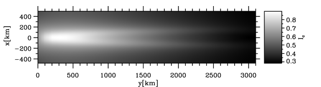
Figure 7: Dark-cored penumbral filament produced by the flux tube considered in this work as seen in continuum intensity at 487.8 nm. The Evershed flow has a velocity of $v_{\rm E}=7$ km s^-1 and induces a temperature excess of $7500$ K within the tube at $y=0$ km.

5 Discussion

5.1 Origin of dark-cored penumbral filaments

Schlichenmaier et al. (1999) studied the radiative cooling of hot flux tubes surrounded by an initially isothermal atmosphere. They found that the tubes cool down quickly in the absence of energy sources, reaching thermal equilibrium with the external medium in only a few tens of seconds. In the case of optically thick tubes (initial temperatures above 10 000 K), a steep cooling front develops and migrates towards the tube axis at constant velocity, while optically thin tubes (initial temperatures below 7500 K) cool more or less homogeneously over their cross sections. In either case, no dark cores would be observed.

Our simulations can be regarded as an extension of the work by Schlichenmaier et al. (1999). The main difference is that we consider a stratified atmosphere consisting of magnetic flux tubes in a stronger ambient field. Under these conditions, the equilibrium temperature distribution is no longer symmetric around the tube axis. We have demonstrated that one such tube would exhibit a central dark core due to the higher density (hence larger opacity) of the plasma within the tube, which moves the $\tau_{\rm R}=1$ level to higher (cooler) layers. The same mechanism produces dark lanes in umbral dots (Schüssler & Vögler 2006) and gappy penumbrae (Spruit & Scharmer 2006), although in these structures the density enhancement is a consequence of overturning convection. In an uncombed penumbra, the density increase is essentially due to the weaker field of the tubes.

It is important to remark, however, that the observations cannot be fully explained without a hot Evershed flow along the tubes. The flow increases the brightness of the flux tube relative to the surroundings and generates the two lateral brightenings of the filaments; in the absence of this energy source, the tubes would actually be darker than their environs.

Borrero (2007) has also been able to reproduce dark-cored filaments using thick penumbral flux tubes in magnetohydrostatic equilibrium. The condition of vertical and horizontal force balance determines the temperature distribution in and around the tubes, given the magnetic field distribution. This results in structures that are hotter than the external medium at the same geometrical height, in good qualitative agreement with our calculations. Borrero (2007) did not identify the source of the heating, but we hypothesize that the higher temperatures required to maintain the tubes in force equilibrium are actually produced by the Evershed flow. To verify this conjecture, the energy and momentum equations must be solved simultaneously in the presence of hot upflows.

5.2 Surplus brightness of the penumbra

An important result of the calculations described in Sect. 4.2 is that the background atmosphere itself is much brighter than it would be in the absence of an Evershed flow. The continuum intensity without flows is only 0.06 $I_{\rm QS}$ (Fig. 4), corresponding to a very cool umbra. In contrast, when a hot upflow is considered, the background shows intensities of up to $\sim$0.7 $I_{\rm QS}$ near the tube (Fig. 7). This enormous difference can explain the surplus brightness of the penumbra relative to the umbra.

The average continuum intensity emerging from the box of Fig. 7 is $\sim$0.5 $I_{\rm QS}$, i.e., slightly smaller than the observed penumbral brightness but of the same order of magnitude. Adjustments of the temperature in the background atmosphere, the geometry of the flux tubes, and/or the boundary conditions for the Evershed flow should easily lead to a closer match.

5.3 Polarimetric signatures of dark-cored penumbral filaments

In this section we investigate the appearance of penumbral flux tubes in polarized light using the results of Sect. 4.2. We have chosen the Fe i line at 630.25 nm to solve the radiative transfer equation because many instruments, including the SOUP magnetograph at the Swedish Solar Telescope (SST) and the polarimeters of the Solar Optical Telescope aboard Hinode, have measured the properties of dark-cored filaments in this line.

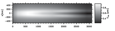
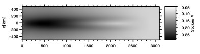
Figure 8: Top: polarization maps of the dark-cored penumbral filament resulting from the simulation of Sect. 4.2 in the Fe i 630.25 nm line. The four panels show the continuum intensity and the wavelength-integrated (unsigned) $Q$, $U$, and $V$ polarization through a 1-m telescope at disk center. The polarization profiles have been normalized to the quiet Sun continuum. Bottom: magnetogram at $+10$ pm from line center and Dopplergram at $\pm 15$ pm from line center.

The four top panels of Fig. 8 show the flux tube as it would be recorded through a 1-m telescope at disk center in continuum intensity and wavelength-integrated Stokes $Q$, $U$, and $V$ polarization, respectively. These maps can be compared with real observations. The dark lane is more prominent in polarized light ($Q$, $U$, and $V$) than in continuum intensity, as observed with Hinode (Bellot Rubio et al. 2007) and the SST (van Noort & Rouppe van der Voort 2008). In total circular polarization, however, the lateral brightenings disappear at too short a distance from the filament head. We believe this is due to the geometry assumed for the flux tube, which never becomes horizontal. Because of the heights attained by the tube, the radiative cooling of the Evershed flow proceeds at a very fast pace. Also, the tube leaves the region of maximum sensitivity of Stokes $V$ comparatively soon, which decreases the circular polarization signal. For these reasons, we expect that a better choice of the tube inclination at large radial distances will produce longer filaments in circular polarization.

The bottom panels of Fig. 8 display a synthetic magnetogram and a Dopplergram of the filament. They have been constructed using the Stokes $V$ profile of Fe i 630.25 nm at $+10$ pm from line center, and the corresponding Stokes $I$ profile at $\pm 15$ pm, respectively. The magnetogram signal is weaker in the dark core than in the lateral brightenings (white means less signal), suggesting weaker and/or more inclined fields. This is exactly what has been inferred from polarimetric measurements of dark-cored filaments (Langhans et al. 2007; Bellot Rubio et al. 2007; van Noort & Rouppe van der Voort 2008). The Dopplergram shows a strong signal in the dark core, indicating the existence of a flow there. Given the disk-center position of the tube and the nearly horizontal inclination of the flow, the Doppler shift is not very conspicuous in this particular example; observations closer to the limb would certainly show stronger signals. In any case, the Dopplergram of Fig. 8 provides the same information as the high-resolution spectroscopic measurements of Bellot Rubio et al. (2005), Rimmele & Marino (2006), and Langhans et al. (2007): the flow appears preferentially in the dark core, not in the lateral brightenings or the adjacent medium.

The qualitative agreement between synthetic and observed parameters is not surprising. As mentioned in Sect. 4.2, a significant fraction of the line-forming region is contained within the flux tube. This means that the physical conditions of the tubes leave their signatures in the Stokes spectra of magnetically sensitive lines. Since the tubes have weaker and more inclined fields, together with strong flows, the polarization profiles emerging from them cannot indicate otherwise. To some extent these arguments justify the conclusions drawn from simple interpretations of polarimetric measurements, but we caution that precise determinations of the magnetic field vector and flow velocity of dark-cored penumbral filaments will require sophisticated inversion techniques such as those used by Borrero et al. (2005) or Jurčak et al. (2007).

6 Conclusions

The heat transfer and radiative transfer calculations presented in this paper support the concept of a penumbra formed by small (but optically thick) magnetic flux tubes that carry hot flows, as deduced from high-resolution observations and spectropolarimetric measurements (see Solanki 2003 and Bellot Rubio 2004 for reviews). Tubes about 250 km in diameter explain not only the existence of dark-cored filaments, but also the surplus brightness of the penumbra; the Evershed flow efficiently heats the plasma outside the tubes, increasing its temperature to values compatible with the observations.

Further improvements of the model should include a more realistic treatment of the magnetic topology of the tubes and the external atmosphere, a better description of convection, and a full 3D solution of the heat transfer equation. In our opinion, however, these improvements will not change the conclusion that the uncombed model is the best representation of the penumbra at our disposal.

Appendix A Magnetic field distribution

We take advantage of the information provided by observations and numerical simulations to constrain the magnetic properties of the model. As mentioned in Sect. 2, the field strength inside the tube, $B_{\rm t}$, must be smaller than in the external medium, $B_{\rm b}$. Also, the inclination of the field in the tube, $\gamma_{\rm t}$, should be larger than in the background far from it, $\gamma_{\rm b}$. These inclinations are measured with respect to the local vertical, as sketched in Fig. 9.

A potential field satisfies the conditions $\nabla\cdot\@vec{B}=0$ and $\nabla\times\@vec{B}=0$. We solve this problem in cylindrical coordinates $r\theta y^{\prime}$, where the $y^{\prime}$-axis coincides with the axis of the tube (Fig. 9). In the tube’s interior ($r<R-\delta$), the field is assumed to be homogeneous and directed along its axis, i.e.,

$$B_{r} = B_{\theta}=0,$$

$$B_{y^{\prime}} = B_{\rm t}.$$ (14)

Variations of the field along the $y^{\prime}$-axis are ignored because they are much smaller than variations perpendicular to the tube’s axis (Borrero et al. 2004). In the background atmosphere, we assume that far from the tube the magnetic field vector is inclined by an angle $\gamma^{\prime}_{\rm b}=90+\gamma_{\rm b}-\gamma_{\rm t}$ with respect to the $z^{\prime}$-axis, and that the field does not depend on $z^{\prime}$. Further, we require continuity of the radial component of the field at $r=R$. Using these boundary conditions, the potential solution for the magnetic field in the external medium ($r>R$) reads

$$B_{r} = B_{\rm b}\,\cos\gamma^{\prime}_{\rm b}\,\sin\theta\,(1-R^{2}/r^{2}),$$

$$B_{\theta} = B_{\rm b}\,\cos\gamma^{\prime}_{\rm b}\,\cos\theta\,(1+R^{2}/r^{2}),$$ (15)

$$B_{y^{\prime}} = B_{\rm b}\,\sin\gamma^{\prime}_{\rm b}$$

Finally, in the current sheet ($r\in[R-\delta,R]$) we demand $B_{\theta}$ and $B_{y^{\prime}}$ to vary linearly, so that

$$B_{r} = 0,$$

$$B_{\theta} = 2\,B_{\rm b}\,\cos\gamma^{\prime}_{\rm b}\,\cos\theta\,\left[r-(R-\delta)\right]/\delta,$$ (16)

$$B_{y^{\prime}} = B_{\rm t}+(B_{\rm b}\,\sin\gamma^{\prime}_{\rm b}-B_{\rm t})\left[(r-(R-\delta)\right]/\delta.$$

With this choice, the magnetic field vector is continuous across the walls of the tube and verifies the condition $\nabla\cdot\@vec{B}=0$.

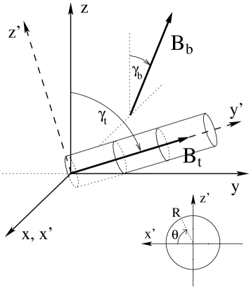
Figure 9: Coordinate systems used in the calculations. The $z$-axis represents the normal to the solar surface. The tube axis is contained in the $yz$-plane. $\gamma_{\rm t}$ and $\gamma_{\rm b}$ are the inclinations of the magnetic field vector in the flux tube ($\@vec{B_{\rm t}}$) and the background atmosphere far from the tube ($\@vec{B_{\rm b}}$), respectively. A new reference system $x^{\prime}y^{\prime}z^{\prime}$ is defined by rotating the $xyz$-system around the $x$-axis until the new $y^{\prime}$-axis coincides with the tube axis. The lower inset shows the cross section of the tube and the angle $\theta$ of the cylindrical coordinate system.

The currents associated with this magnetic field are non-zero only in $r\in[R-\delta,R]$ and can be expressed as

$$j_{\rm r} = 0,$$

$$j_{\theta} = -\frac{B_{\rm b}\sin\gamma^{\prime}_{\rm b}-B_{\rm t}}{\mu\delta}$$ (17)

$$j_{y^{\prime}} = \frac{2\,B_{\rm b}}{\mu\delta}\,\left[2-\frac{R-\delta}{r}\right]\,\cos\gamma^{\prime}_{\rm b}\cos\theta,$$

$\mu$ being the magnetic permeability in vacuum. The current in the direction of the tube axis, $j_{y^{\prime}}$, is proportional to the jump of the vertical component of the magnetic field vector. It reaches a maximum at $z^{\prime}=0$ and vanishes at the top and bottom of the tube (where $\theta=90^{\circ}$ and $\theta=270^{\circ}$).

References

- (1) Beck, C. 2008, A&A, 480, 825
- (2) Bellot Rubio, L.R. 2004, Reviews in Modern Astronomy, 17, 21
- Bellot Rubio (2007) Bellot Rubio, L.R. 2007, in Highlights of Spanish Astrophysics IV, ed. F. Figueras et al. (Dordretch: Springer), 271
- Bellot Rubio et al. (2004) Bellot Rubio, L.R., Balthasar, H., & Collados, M. 2004, A&A, 427, 319
- (5) Bellot Rubio, L.R., Langhans, K., Schlichenmaier, R. 2005, A&A, 443, L7
- Bellot Rubio et al. (2006) Bellot Rubio, L. R., Schlichenmaier, R., & Tritschler, A. 2006, A&A, 453, 1117
- Bellot Rubio et al. (2007) Bellot Rubio, L. R., et al. 2007, ApJ, 668, L91
- (8) Borrero, J.M. 2007, A&A, 471, 967
- Borrero et al. (2007) Borrero, J. M., Bellot Rubio, L. R., Müller, D. A. N. 2007, ApJ, 666, L133
- Borrero et al. (2005) Borrero, J. M., Lagg, A., Solanki, S. K., & Collados, M. 2005, A&A, 436, 333
- (11) Borrero, J.M., Rempel, M., & Solanki, S.K. 2006, in Solar Polarization IV, ed. R. Casini, & B.W. Lites, ASP Conf. Ser., 358, 19
- (12) Borrero, J.M., Solanki, S.K., Bellot Rubio, L.R., Lagg, A., Mathew, S.K. 2004, A&A, 422, 1093
- Collados et al. (1994) Collados, M., Martínez Pillet, V., Ruiz Cobo, B., del Toro Iniesta, J.C., & Vázquez, M. 1994, A&A, 291, 622
- Cox & Giuli (1968) Cox, J.P., & Giuli, R.T. 1968, Principles of Stellar Structure, (New York: Gordon and Breach)
- Heinemann et al. (2007) Heinemann, T., Nordlund, Å., Scharmer, G. B., & Spruit, H. C. 2007, ApJ, 669, 1390
- (16) Ichimoto, K., et al. 2007, PASJ, 59, S593
- (17) Jurčak, J., et al. 2007, PASJ, 59, S601
- Langhans et al. (2007) Langhans, K., Scharmer, G. B., Kiselman, D., Löfdahl, M. G. 2007, A&A, 464, 763
- (19) Levermore, C.D., & Pomraning, G.C. 1981, ApJ, 248, 321
- (20) Kopecký, M. & Kuklin, G.V. 1969, Sol. Phys., 6, 241
- (21) Mihalas, D. 1978, Stellar Atmospheres, (San Francisco: Freeman and Co.)
- (22) Moreno-Insertis, F., Schüssler. M., & Glampedakis, K. 2002, A&A, 388, 1022
- Müller et al. (2002) Müller, D. A. N., Schlichenmaier, R., Steiner, O., & Stix, M. 2002, A&A, 393, 305
- Rimmele (2008) Rimmele, T. 2008, ApJ, 672, 684
- Rimmele & Marino (2006) Rimmele, T., & Marino, J. 2006, ApJ, 646, 593
- (26) Rouppe van der Voort, L.H.M., Löfdahl, M.G., Kiselman, D., Scharmer, G.B. 2004, A&A, 414, 717
- (27) Sainz Dalda, A., & Bellot Rubio, L.R. 2008, A&A, 481, L21
- Scharmer et al. (2002) Scharmer, G.B., Gudiksen, B.V., Kiselman, D., Löfdahl, M.G., & Rouppe van der Voort, L.H.M. 2002, Nature, 420, 151
- (29) Scharmer, G.B., & Spruit, H.C. 2006, A&A, 460, 605
- Schlichenmaier (2002) Schlichenmaier, R. 2002, AN, 323, 303
- Schlichenmaier (2003) Schlichenmaier, R. 2003, in Current Theoretical Models and Future High Resolution Solar Observations: Preparing for ATST, ASP Conf. Ser., 286, 211
- Schlichenmaier & Schmidt (2000) Schlichenmaier, R., & Schmidt, W. 2000, A&A, 358, 1122
- (33) Schlichenmaier, R., & Solanki, S.K. 2003, A&A, 411, 257
- (34) Schlichenmaier, R., Jahn, K., & Schmidt, H.U. 1998, A&A, 337, 897
- (35) Schlichenmaier, R., Bruls, J.H.M.J., & Schüssler, M. 1999, A&A, 349, 961
- (36) Schüssler, M., & Vögler, A. 2006, ApJ, 641, L73
- (37) Solanki, S.K. 2003, A&A Rev., 11, 153
- (38) Solanki, S.K., & Montavon C.A.P., 1993, A&A, 275, 283
- (39) Spruit, H.C. 1977, Sol. Phys., 55, 3
- (40) Spruit, H.C., & Scharmer, G.B. 2006, A&A, 447, 343
- Stanchfield et al. (1997) Stanchfield, D.C.H., Thomas, J.H., & Lites, B.W. 1997, ApJ, 477, 485
- (42) Sütterlin, P., Bellot Rubio, L.R., & Schlichenmaier, R. 2004, A&A, 424, 1049
- Title et al. (1993) Title, A.M., Frank, Z.A., Shine, R.A., Tarbell, T.D., Topka, K.P., Scharmer, G., & Schmidt, W. 1993, ApJ, 403, 780
- Tritschler et al. (2007) Tritschler, A., Müller, D. A. N., Schlichenmaier, R., & Hagenaar, H. J. 2007, ApJ, 671, L85
- van Noort & Rouppe van der Voort (2008) van Noort, M.J., & Rouppe van der Voort, L.H.M. 2008, A&A, in press, [arXiv:0805.4296]
- Westendorp Plaza et al. (2001) Westendorp Plaza, C., del Toro Iniesta, J.C., Ruiz Cobo, B., & Martínez Pillet, V. 2001, ApJ, 547, 1148