Fractal analysis of the dark matter and gas distributions in the Mare-Nostrum universe

Abstract:

We develop a method of multifractal analysis of $N$-body cosmological simulations that improves on the customary counts-in-cells method by taking special care of the effects of discreteness and large scale homogeneity. The analysis of the Mare-Nostrum simulation with our method provides strong evidence of self-similar multifractal distributions of dark matter and gas, with a halo mass function that is of Press-Schechter type but has a power-law exponent $-2$, as corresponds to a multifractal. Furthermore, our analysis shows that the dark matter and gas distributions are indistinguishable as multifractals. To determine if there is any gas biasing, we calculate the cross-correlation coefficient, with negative but inconclusive results. Hence, we develop an effective Bayesian analysis connected with information theory, which clearly demonstrates that the gas is biased in a long range of scales, up to the scale of homogeneity. However, entropic measures related to the Bayesian analysis show that this gas bias is small (in a precise sense) and is such that the fractal singularities of both distributions coincide and are identical. We conclude that this common multifractal cosmic web structure is determined by the dynamics and is independent of the initial conditions.

1 Introduction

The large scale structure of the Universe can be described as a “cosmic web” formed by matter sheets, filaments and nodes. This type of structure was initially proposed in connection with simplified but insightful models of the cosmic dynamics [1] and has been since confirmed by galaxy surveys and $N$-body cosmological simulations [2]. Cosmological simulations have been especially helpful in testing models of structure formation. In a sense, they have been complementary to observations, since observations are biased towards the luminous matter, while simulations have fully considered the evolution of the dark matter, which is actually the dominant component. In fact, many simulations only consider dark matter, in particular, non-baryonic cold dark matter, whose dynamics is simplest to simulate and gives rise to cosmic structure that is in accord with observations. However, due to the advances in parallel computing, the development of efficient codes, and the availability of more powerful computers, the scope of $N$-body simulations has recently changed: now it is possible to simulate the combined dynamics of the non-baryonic dark matter and the baryon gas in large cosmological volumes and with relatively good resolution.

We analyse here the data output of a recent large cosmological simulation of the combined dark matter and gas dynamics, namely, a simulation of the cosmic evolution of $1024^{3}$ dark-matter particles and an equal number of gas particles carried out by the Mare-Nostrum supercomputer in Barcelona. This dataset has already been analysed by the researchers in charge of the Mare-Nostrum universe project [3, 4, 5]. Here, we are interested in a particular aspect of the dark matter and gas distributions: their geometry and, specifically, their fractal geometry.

Fractal geometry [6] is the geometry of sets or distributions that have noticeable geometrical features on ever decreasing scales. It is related to scale invariance and indeed appears in nonlinear dynamical systems in which the dynamics is characterized by the absence of reference scales. This is the case of the dynamics of collision-less cold dark matter (CDM), only subjected to the gravitational interaction. Therefore, the cosmic web produced by this type of dynamics has fine structure and it is, arguably, statistically self-similar. We can reasonably assume that the cosmic web is a multifractal attractor of the gravitational dynamics. This model is supported by the results of CDM simulations [7, 8, 9, 10, 11]. Although the gas dynamics is more complex (due to the gas pressure, etc), the gas takes part in the nonlinear dynamics of structure formation and can also have a multifractal attractor. Indeed, scaling laws in the distribution of galaxies have a long history, which has been reviewed in Refs. [12, 13, 14]. Therefore, it is interesting to compare the scaling laws in the distribution of gas with the scaling laws in the distribution of dark matter.

Fractal models of the cosmic structure can only be valid in a range of scales, whose upper cutoff is the scale of homogeneity. Its value has been the subject of considerable debates and still is controversial [13, 14]. In contrast, the lower cutoff to scaling has attracted less attention. In fact, the CDM gravitational dynamics does not introduce any small reference scale that can play the rôle of a lower cutoff, but the gas dynamics introduces the Jeans length. This length is not a fixed reference scale, for it depends on the local thermodynamical parameters. In any event, one should expect that the lower cutoff to scaling in the dark matter distribution is smaller than the lower cutoff appropriate for the distribution of galaxies. However, the opposite seems to be true if one compares galaxy surveys with the results of cosmological simulations, since the latter exhibit reduced scaling ranges, even in dark matter only simulations. Peebles has included this problem in his list of anomalies in standard cosmology [15]. In his words: “scale-dependent biasing seems an awkward way to account for the power-law forms of the low order galaxy position correlation functions.”

One can be inclined to place more trust in the scaling range found in galaxy surveys: cosmological simulations allow one to obtain better statistics but they are not free of systematic errors that affect an important range of the smaller scales. Indeed, it has been long known that $N$-body simulations are not fully reliable on scales smaller than the mean particle spacing $N^{-1/3}$ [16, 17]. In spite of the ever-growing value of $N$, the range of scales between the scale $N^{-1/3}$ and the homogeneity scale is still rather small. In the Mare-Nostrum universe, this scale range spans a factor of 30 (see Sects. 2 and 3). Our goal is to demonstrate multifractality of the dark matter and gas distributions in the valid scale range. Furthermore, given that this scale range is small, we devise a method to correct for discreteness effects and thus extend the valid range to smaller scales, obtaining a reasonable scaling range. We also intend to test if the dark matter and gas distributions constitute a unique distribution or to what extent they differ. Hence, we make a model of fractal biasing.

We describe our method of coarse multifractal analysis by counts in cells and define the basic objects (halos) in Sect. 2. In our method, the scale of homogeneity is explicitly introduced to calculate the multifractal spectrum (Sect. 2.1). In Sub-sect. 2.2, we show how to obtain the main features of this spectrum and how they are influenced by discreteness and large scale homogeneity. In Sect. 3, we apply our method to the zero-redshift particle distributions of the Mare-Nostrum universe: (i) we obtain the halo mass functions and discuss its relation to the Press-Schechter mass function in Sect. 3.1; (ii) we obtain the multifractal spectra and discuss their relevance in regard to other geometrical studies of the cosmic web in Sect. 3.2; and (iii) we demonstrate scaling and compute sound values of the correlation dimensions in Sect. 3.3. The similarity of the results corresponding to the gas and the dark matter suggests that both distributions are identical and shows the need of precise statistical methods to discriminate between them (Sect. 4). Since the cross-correlations cannot give a definite answer (Sub-sect. 4.1), we develop an effective Bayesian analysis (Sub-sect. 4.2) which we apply to various cell distributions (Sub-sect. 4.3). This analysis connects with the thermodynamic entropy of mixing (Sub-sect. 4.4). Therefore, we study the application of entropic measures to discriminating between mass distributions, and we study the connection of entropies in the continuum limit with the multifractal spectrum (Sect. 5). Finally, we discuss our results (Sect. 6).

A note on notation: we use frequently the asymptotic signs $\sim$ and $\approx$; for example, $f(x)\sim g(x)$ or $f(x)\approx g(x)$ (often without making explicit the independent variable $x$). The former means that the limit of $f(x)/g(x)$ is finite and non-vanishing when $x$ approaches some value (which can be zero or infinity), while the latter means, in addition, that the limit is one. We also use the sign $\simeq$, which only refers to imprecise numerical values (with unspecified errors).

2 Methods of data analysis

The Mare-Nostrum cosmological simulation is described by Gottlöber et al [3]. It assumes a spatially flat concordance model with parameters $\Omega_{\Lambda}=0.7$, $\Omega_{\bar{\rm m}}=0.3$, $\Omega_{\rm bar}=0.045$, Hubble parameter $h=0.7$, and initial spectrum with spectral index $n=1$, in a comoving cube of 500 $h^{-1}$ Mpc edges. The Gadget-2 code [18] simulated the evolution of dark matter and gas from redshift $z=40$ to $z=0$. Both dark matter and gas are resolved by $1024^{3}$ particles, respectively, which results in a mass of $8.24\cdot 10^{9}\,h^{-1}\,M_{\odot}$ per dark-matter particle and a mass of $1.45\cdot 10^{9}\,h^{-1}\,M_{\odot}$ per gas particle. The Gadget-2 code implements polytropic (adiabatic) evolution of the gas. It can also include dissipation due to radiation or conduction, but these processes have not been included in the Mare-Nostrum simulation. Nevertheless, the code always includes an artificial viscosity to take care of shock waves.

The Mare-Nostrum universe consists of 135 evenly spaced snapshots. For our statistical analysis, we only need the $z=0$ snapshot, in which the homogeneity scale is largest and the structures are most developed. The large size of a Mare-Nostrum universe snapshot makes it unwieldy, so it is convenient (and almost necessary) to analyse it in terms of compound structures, namely, halos, rather than analysing the full particle distributions. The Mare-Nostrum universe researchers [3, 4, 5] use a friends-of-friends algorithm to define halos, and then they study the distribution and features of those halos. However, we prefer the method of counts in cells, more suitable for studying the continuum limit and the scaling properties of particle distributions. Therefore, our elementary objects (halos) are cells with constant size but variable mass. The definition of elementary objects in distributions with fine structure (fractals) is arbitrary to a high degree, being actually tied to the measurement or analysis technique. The definition of elementary objects by coarse graining and, in particular, their definition as cells in a mesh, is very convenient [10]. In absence of a reference scale, the appropriate cell size (the coarse-graining scale) is arbitrary, and there is no clear distinction between inner and outer structure. However, an $N$-point fractal sample, as a finite point distribution, has a reference scale, namely, the discreteness scale $N^{-1/3}$, which allows us to properly define the size of elementary objects.

At any rate, the cell size must be considered a running scale. The use of a running cell size is useful, for example, to distinguish the nonlinear scales where structure formation takes place from the linear scales where the initial conditions are preserved: as the cell size enters in the range of the latter scales, the fluctuations of the counts in cells are reduced to small Gaussian fluctuations. This homogeneity scale is actually the only real scale in the cosmic CDM dynamics, although it is not a sharp scale and, besides, it grows with time.

The method of counts in cells is also suitable for comparing the gas distribution with the dark matter distribution, by comparing the respective counts, for a given cell size. Of course, we must devise methods to provide these comparisons with statistical meaning. We defer further description of our methods to Sect. 4. However, we advance that our main procedure naturally connects with the description of multifractals in terms of Rényi dimensions.

In summary, our basic assumption is that the Mare-Nostrum particle distributions represent continuous mass distributions with fine structure but which are homogeneous on the large scales. In particular, we expect continuous distributions of cosmic web type, which have various kinds of density singularities produced by gravitational collapse. The properties of these singularities can be deduced by suppressing the effects of discreteness. We introduce in next sub-section methods of multifractal analysis geared to the relevant type of singular distributions. In sub-section 2.2, we study the influence of the discreteness scale and the homogeneity scale on the features of the coarse multifractal spectrum.

2.1 Counts in cells and coarse multifractal analysis

Let us assume that a mesh of cells is placed in the sample region (the simulation cube). In the method of counts in cells, (fractional) statistical moments are defined as

$$M_{q}=\sum_{i}\left(\frac{n_{i}}{N}\right)^{q}=\sum_{n>0}N(n)\left(\frac{n}{N}\right)^{q},$$ (1)

where the index $i$ refers to non-empty cells, $n_{i}$ is the number of points (particles) in the cell $i$, $N=\sum_{i}n_{i}$ is the total number of points, and $N(n)$ is the number of cells with $n$ points. The second expression involves a sum over cell populations and it is more useful than the sum over individual cells, because the range of $n$ is much smaller (when the cell size is small). $M_{0}$ is the number of non-empty cells and $M_{1}=1$. We understand the latter as a mass normalization, namely, the mass in cell $i$ is $n_{i}/N$ and the total mass is one, such that the mass distribution can be interpreted as a probability distribution (the physical masses of gas or dark-matter particles play no rôle in the statistical analysis). There is an alternate definition of $q$-moments:

$$\mu_{q}=\langle\rho^{q}\rangle=\sum_{n>0}\frac{N(n)}{M_{0}}\left(\frac{n}{NV}\right)^{q}=\frac{M_{q}}{V^{q}M_{0}}\,,$$ (2)

where $V$ is the cell’s volume, $N(n)/M_{0}$ is the fraction of cells that contain $n$ points, and $\rho=n/(NV)$ is the density in those cells. With this definition, $\mu_{0}=1$ while $\mu_{1}$ is not fixed. We notice that the moments with positive integer $q$ ($M_{q}$ or $\mu_{q}$, $q\in\mathbb{N}$) are sufficient for regular distributions, but we cannot impose this restriction here ($q\in\mathbb{R}$).

In regular distributions, the mass contained in any cell is proportional to its volume $V$, in the continuum limit $V\rightarrow 0$. Therefore, $M_{q}\sim V^{q-1}$. However, we consider singular distributions such that their $q$-moments are non-trivial power laws of $V$ in the continuum limit, namely, distributions such that one can define [19] the exponents

$$\tau(q)=3\lim_{V\rightarrow 0}\frac{\log M_{q}}{\log V}\,,\;q\in\mathbb{R}\,.$$ (3)

These distributions are called multifractals. Of course, the numerical evaluation of the limit in Eq. (3) is not feasible and one must be satisfied with finding a constant value of the quotient for sufficiently small $V$, that is, in a sufficiently long range of negative values of $\log V$ (a range of scales). In fact, the exponent is normally defined as the slope of the plot of $\log M_{q}$ versus $\log V$, and its value is found by numerically fitting that slope, supposing that a meaningful fit is possible.

A multifractal is also characterized by a set of local dimensions: the local dimension at one point says how the mass grows from that point outwards. Every set of points with a given local dimension $\alpha$ constitutes a fractal set with dimension $f(\alpha)$. In terms of $\tau(q)$, the spectrum of local dimensions is given by

$$\alpha(q)=\tau^{\prime}(q)\,,\quad q\in\mathbb{R}\,,$$ (4)

and the spectrum of fractal dimensions $f(\alpha)$ is given by the Legendre transform

$$f(\alpha)=q\,\alpha-\tau(q)\,.$$ (5)

The spectrum of fractal dimensions is convex upwards and fulfills $f(\alpha)\leq\alpha$. The fractal dimension $f(\alpha)$ reaches the local dimension $\alpha$ at $q=1$ [note that Eq. (3) gives $\tau(1)=0$]. The set of singularities with $f(\alpha_{1})=\alpha_{1}$ contains the bulk of the mass and is called the “mass concentrate.”

In addition to the exact exponent $\tau(q)$ (3), we define, for a given cell size, the coarse exponent

$$\tau(q)=3\frac{\log(M_{q}/V_{0}^{q-1})}{\log(V/V_{0})}\,,$$ (6)

where $V$ is the cell size and $V_{0}$ is the homogeneity scale, such that the density is homogeneous and $M_{q}\approx V^{q-1}$ for $V>V_{0}$. The coarse exponent depends on both $V$ and $V_{0}$, but this dependence vanishes if $V\ll V_{0}$ (assuming that the limit $V\rightarrow 0$ exists). The introduction of the homogeneity scale in Eq. (6) improves the definition used in Ref. [10] for the GIF2 simulation, where no $V_{0}$ is introduced (equivalent to setting $V_{0}=1$). Given that the Mare-Nostrum universe cube has 500 $h^{-1}\!$ Mpc edges, much longer than the 110 $h^{-1}\!$ Mpc edges of the GIF2 simulation cube, it is important now to take the transition to homogeneity into account in the definition of the coarse exponent, if we want it to be a good approximation of the limit (3) for moderately small $V$.

The homogeneity scale $V_{0}$ can be found as the scale of crossover to homogeneity in the scaling of statistical moments (Sect. 3.3). We can also estimate it as the coarse-graining scale such that the mass fluctuations are smaller than, say, 10%; namely, we define it as the scale such that $\mu_{2}=1.1$. Thus, we find that the scale of homogeneity is about 1/16th of the edge of the cube, namely, about 30 $h^{-1}$ Mpc. This value is similar to the value of the GIF2 homogeneity scale found in Ref. [10], where it is calculated from the crossover in the scaling of moments.

Besides the multifractal spectrum $f(\alpha)$, it is useful to define the spectrum of Rényi dimensions [19]

$$D_{q}=\frac{\tau(q)}{q-1}\,.$$ (7)

They have an information-theoretic meaning, which will be explained in detail in Sect. 5. In particular, the dimension of the mass concentrate $\alpha_{1}=f(\alpha_{1})=D_{1}$ is also called the entropy dimension. $D_{0}$ coincides with the maximum value of $f(\alpha)$ and with the box-counting dimension of the distribution’s support, while $D_{2}=\tau(2)$ is the correlation dimension. In the homogeneous regime, $M_{q}\approx V^{q-1}$ and $D_{q}=3$ for any $q$. In a uniform fractal (a unifractal or monofractal) $D_{q}$ is also constant but smaller than three. In general, $D_{q}$ is a non-increasing function of $q$.

2.2 Features of the coarse multifractal spectrum

Here, we examine the features of the multifractal spectrum obtained from the coarse exponent defined by Eq. (6).

In a multifractal, the cell size $V$ is, of course, irrelevant, as long as $V$ is sufficiently smaller than the homogeneity scale $V_{0}$. However, the intrinsic discreteness of a multifractal sample (a finite point distribution) gives rise to another scale, namely, the size of the cell such that there is one point per cell on average ($V=N^{-1}$). This scale represents the minimal scale at which the distribution can be consistently considered continuous. In the initial stages of an $N$-body simulation, when there are only very small deviations from the one-particle-per-cell average, it is obvious that it makes no sense to consider smaller scales. Furthermore, the dynamics of gravitational collapse is deeply distorted on volumes $V<N^{-1}$, so the resulting particle clusters do not represent the structures that result from the collapse of a continuous medium [16, 17]. As a coarse-graining scale, the volume $V=N^{-1}$ produces the largest variety of masses of coarse-grained objects in $N$-body cosmological simulations [10]. Thus, this cell size provides us with a sort of master cell distribution that characterizes the multifractal sample. Whenever we mention halos, we refer to non-empty master cells, preferably with a considerable number of particles. Since the number of dark-matter or gas particles in the Mare-Nostrum universe is a perfect cube and, indeed, a power of two, the master cell distributions are easily obtained.

Ref. [10] shows that the mass function of halos in the GIF2 simulation follows the power law $N(m)\sim m^{-2}$, except at the large mass end, where it decays faster. This power law derives from an approximation of the multifractal spectrum, namely, $f(\alpha)\approx\alpha$, and therefore represents the mass concentrate of the multifractal. In contrast, the master cell distribution contains no information of the matter distribution in voids (zones with $\alpha>3$), because they are empty [10, 11]. Hence, a part of the multifractal spectrum is missing even at this scale. As $V$ shrinks, the multifractal spectrum is reduced further.

The length scale that corresponds to $V=N^{-1}$ in the Mare-Nostrum simulation, namely, $l=N^{-1/3}=2^{-10}$, is only a factor $2^{6}=64$ smaller than $l_{0}=V_{0}^{1/3}=2^{-4}$. This is the largest scaling range that could be attainable in principle, despite the large number of particles. In fact, close to the large scale end, at $l_{0}=2^{-4}$, the coarse multifractal spectrum is influenced by homogeneity, whereas close to the opposite end it is influenced by discreteness. Surely, the best estimation of the real spectrum is to be found somewhere in between. Let us study in detail the change of the features of the coarse multifractal spectrum with scale.

For a given coarse-graining scale, we calculate with Eqs. (1) and (6) the exponent $\tau(q)$, and hence we calculate the coarse multifractal spectrum through the Legendre transform given by (4) and (5). The lower end of this spectrum corresponds to the limit $q\rightarrow\infty$, that is to say, to the cell(s) with maximum number of particles:

$$\alpha_{{\rm min}}=\lim_{q\rightarrow\infty}\alpha(q)=3\frac{\log[n_{{\rm max}}/(NV_{0})]}{\log(V/V_{0})}\,,$$ (8)

$$f(\alpha_{{\rm min}})=-3\frac{\log[N(n_{{\rm max}})\,V_{0}]}{\log(V/V_{0})}\,.$$ (9)

Since $\alpha_{{\rm min}}$ is the local dimension of the strongest singularity, it changes little with the scale, unless we approach homogeneity ($V\to V_{0}$), which implies that $\alpha_{{\rm min}}\to 3$. Usually, $N(n_{{\rm max}})=1$, namely, there is only one cell with the maximum number of particles. Therefore, the choice $V_{0}=1$, which disregards the effect of homogeneity, implies that $f(\alpha_{{\rm min}})=0$. However, any $V_{0}<1$, like our present setting $V_{0}=1/4096$, implies that the fractal dimension $f(\alpha_{{\rm min}})$ is negative!

Intuitively, negative fractal dimensions seem meaningless, but they often arise in the study of random multifractals. The origin of negative fractal dimensions has been discussed by Mandelbrot [20]. In brief, the coarse fractal dimension of a set of singularities in a random multifractal is proportional to the logarithm of their number, but the expected value of this number can be smaller than one. Therefore, sets of singularities with negative fractal dimension are probably empty. In our case, by setting $V_{0}$ to a fraction of the total volume, the number of singularities with given $\alpha$ in cubes of size $V_{0}$ fluctuates and these fluctuations are more important for values of $\alpha$ such that there are few singularities with that $\alpha$ in the whole simulation box. Thus, it is convenient to “average” over the $V_{0}^{-1}=4096$ cubes and consider at once the 4096 singularities with smallest $\alpha$, truncating the negative values of the multifractal spectrum.

In analogy with the lower end of the spectrum of local dimensions, we can deduce that its upper end corresponds to the limit $q\rightarrow-\infty$, that is, to the set of cells with one particle (assuming that $V$ is not so large that there are none). In fact,

$$\alpha_{{\rm max}}=\lim_{q\rightarrow-\infty}\alpha(q)=-3\frac{\log(NV_{0})}{\log(V/V_{0})}\,,$$ (10)

$$f(\alpha_{{\rm max}})=-3\frac{\log[N(1)V_{0}]}{\log(V/V_{0})}\,.$$ (11)

Notice that the master cell distribution has $\alpha_{{\rm max}}=3$ and, therefore, its spectrum is limited to non-void zones ($\alpha\leq 3$). The value of $\alpha_{{\rm max}}$ increases for cell sizes $V>1/N$, as voids begin to be sampled. For sufficiently large $V$, $N(1)$ decreases and approaches $1/V_{0}=4096$ (only one cell with one particle per each cube of size $V_{0}$). Then, $f(\alpha_{{\rm max}})$ decreases to zero. At this scale, we have the complete (positive) multifractal spectrum in the region $\alpha>3$, corresponding to voids, and the distribution can be considered continuous over the entire range of $\alpha$ [we always discard the negative values of $f(\alpha)$].

The total span of the spectrum is

$$\alpha_{{\rm max}}-\alpha_{{\rm min}}=-3\frac{\log(n_{{\rm max}}/n_{{\rm min}})}{\log(V/V_{0})}\,,$$

where $n_{{\rm min}}\equiv 1$ in the relevant range of $V$. Naturally, the largest span is reached when the spectrum is complete in the region $\alpha>3$. For the Mare-Nostrum universe, we indeed show in Sect. 3.2 that we obtain, by choosing $V$ to be the largest value such that $f(\alpha_{{\rm max}})\geq 0$, the largest span of dimensions $\alpha$ and a good estimate of the full multifractal spectrum. For larger values of $V$, as the transition to homogeneity begins, $n_{{\rm min}}$ grows and approaches $n_{{\rm max}}$, with the consequent contraction of the span of the spectrum.

Scale invariance implies that the multifractal spectra at different coarse-graining scales coincide in their respective ranges $[\alpha_{{\rm min}},\alpha_{{\rm max}}]$, where $\alpha_{{\rm min}}$ is roughly constant but $\alpha_{{\rm max}}$ increases with the scale. However, the under-sampling of low density regions that causes the truncation of the spectrum at $\alpha_{{\rm max}}$ also causes deviations from the true spectrum close to $\alpha_{{\rm max}}$. These deviations must be corrected. We see how to do it for the Mare-Nostrum multifractal spectra in Sects. 3.2 and 3.3.

Regarding the master cell distribution and assuming for it the simple mass function $N(n)=N(1)/n^{2}$, we can deduce interesting consequences about the corresponding coarse multifractal spectrum. First, we calculate, according to Eq. (1),

$$M_{0}=\sum_{n=1}^{n_{{\rm max}}}N(n)\approx N(1)\sum_{n=1}^{\infty}\frac{1}{n^{2}}=N(1)\,\frac{\pi^{2}}{6}\;.$$

Since this sum is just the number of non-empty cells, we deduce that the fraction of non-empty cells containing one particle is $N(1)/M_{0}\approx 6/\pi^{2}=0.61$. Thus, the full distribution $N(n)$ is determined by just the number of empty cells. Furthermore, from the expression

$$M_{1}=\sum_{n=1}^{n_{{\rm max}}}N(n)\frac{n}{N}\approx\frac{N(1)}{N}\ln n_{{\rm max}}\;,$$ (12)

and the condition $M_{1}\equiv 1$ we can determine $n_{{\rm max}}$. Then, the dimension of the mass concentrate $\alpha_{1}=f(\alpha_{1})$ is

$$\alpha_{1} = \tau^{\prime}(1)=\frac{3}{\ln(V/V_{0})}\left(\left.\frac{dM_{q}}{dq}\right|_{q=1}-\ln V_{0}\right)$$

$$= \frac{3}{\ln(V/V_{0})}\left(\sum_{n=1}^{n_{{\rm max}}}N(n)\frac{n}{N}\ln\frac{n}{N}-\ln V_{0}\right)$$

$$\approx \frac{3}{\ln(V/V_{0})}\,\left(\frac{\ln n_{{\rm max}}}{2}-\ln(NV_{0})\right).$$

This dimension is the arithmetic mean of the general values of $\alpha_{{\rm min}}$ in Eq. (8) and $\alpha_{{\rm max}}$ in Eq. (10).

3 Multifractal analysis of the dark matter and gas distributions

We now present the results of the multifractal analysis of the Mare-Nostrum universe $z=0$ snapshot, beginning with the halo mass functions given by the counts in the master cell distributions (Sect. 3.1). In Sect. 3.2, we study the multifractal spectra in the range of scales covering several powers of two, namely, from $l=2^{-12}$ to $l=2^{-7}$. The latter scale is the smallest scale (among the powers of two) such that $N(1)<4096$ and therefore the spectrum corresponding to voids is complete. On smaller scales, namely, between $l=2^{-12}$ and $l=2^{-8}$, the high-$\alpha$ ends of the coarse spectra deviate from the true spectrum due to under-sampling of the low density regions. In Sect. 3.3, we propose to correct for under-sampling by removing the erroneous ends of the spectrum. Thus, we can demonstrate scale invariance in the longest possible range.

3.1 Mass functions

In Fig. 1 are plotted the halo mass functions of dark-matter and gas, obtained from the counts in the master cell distributions. The mass $m$ is actually defined as the number of particles, for simplicity. Both mass functions follow the power law $N(m)\sim m^{-2}$ over a considerable range of $m$: least-squares fits in the $\log_{2}m$ range from 0 to 9 yield slopes $-2.07$, for the dark matter, and $-2.12$, for the gas.

Figure 1: Log-log plots of the number of halos $N$ versus their mass $m$ (number of particles) at coarse-graining scale $1024^{-1}$, in the case of dark matter (left) and gas (right).

There are $156\hskip 1.0pt272\hskip 1.0pt463$ cells with one dark-matter particle and $170\hskip 1.0pt546\hskip 1.0pt782$ cells with one gas particle in the master cell distribution. According to Eq. (11), the fractal dimensions of the sets with $\alpha_{{\rm max}}=3$ are $f(\alpha_{{\rm max}})=2.54$ and $2.56$, for the dark matter and gas, respectively. The cell with the largest proportion of dark matter has $20\hskip 1.0pt658$ dark-matter particles and it also has the largest proportion of gas, namely, $19\hskip 1.0pt200$ gas particles; all the particles together form the most massive halo. The corresponding values of $\alpha_{{\rm min}}$, according to Eq. (8), are $0.61$ and $0.63$, respectively. However, Eq. (9) yields negative values of $f(\alpha_{{\rm min}})$, which we do not consider. We compute directly from Eqs. (4), (5) and (6) that the values of $\alpha$ such that $f(\alpha)=0$ are $0.91$ (dark matter) and $0.95$ (gas).

We have seen in the preceding section that the value of $\alpha_{1}$ corresponding to the master cell distribution can be estimated as the arithmetic mean of $\alpha_{{\rm min}}$ and $\alpha_{{\rm max}}=3$. Whether we use $\alpha_{{\rm min}}\simeq 0.6$ or $\alpha_{{\rm min}}\simeq 0.9$, this estimation yields smaller values than the actual values, which are $2.22$ (dark matter) and $2.29$ (gas). On the other hand, the estimation $m_{{\rm max}}=\exp[N/N(1)]$, deduced by making $M_{1}=1$ in Eq. (12), yields 967 and 542, respectively, well below the real values (see Fig. 1). The problem is that the power law is modified at the large mass end, as we can perceive in Fig. 1. On the one hand, at the large mass end, the values of $N(m)$ are so small that there are many values of $m$ for each value of $N$; on the other hand, $N$ as a function of the average of the corresponding values of $m$ decays faster than a power law. In fact, the above estimated values of $m_{{\rm max}}$ actually mark the ends of the power laws, instead of the ends of the large masses.

We can improve the fit of the mass function by modelling the large mass end of the power law. For this, we can take inspiration from the Press-Schechter mass function,

$$N(m)\propto\left(\frac{m}{m_{*}}\right)^{n/6-3/2}\exp\left[-\left(\frac{m}{m_{*}}\right)^{n/3+1}\right],$$ (13)

where $n>-3$ is the spectral index of the initial power spectrum and $m_{*}$ stands for the large-mass cutoff. In fact, the agreement between the power-law parts of Eq. (13) and of the found mass function demands $n\rightarrow-3$. Therefore, we take

$$N(m)\approx N(1)\,m^{-2}\exp\left[-\left(\frac{m}{m_{*}}\right)^{\!\epsilon}\,\right],$$ (14)

where $\epsilon>0$ is to be fitted, as well as $m_{*}$. The latter can be deduced from the condition $M_{1}=1$; namely,

$$M_{1} \approx \frac{N(1)}{N}\sum_{m=1}^{\infty}\frac{\exp[-(m/m_{*})^{\epsilon}]}{m}$$

$$\approx -\frac{N(1)}{N}\int_{m=1}^{\infty}dm\,\frac{\exp[-(m/m_{*})^{\epsilon}]}{m}\approx\frac{N(1)}{N}\,\ln m_{*}\,.$$

It is independent of $\epsilon$, and coincides with the value given by Eq. (12) if we identify $m_{{\rm max}}$ there with $m_{*}$. This identification is natural, because the exponential form (14) is just one way of introducing a mass cutoff that is more adequate than the sharp cutoff used in Eq. (12). We can see why the above quoted values of $m_{{\rm max}}$, below 1000, actually mark the end of the power laws. The new values of $m_{{\rm max}}$ are obtained from expression (14) by requiring $N(m_{{\rm max}})=1$. Thus, this model raises the estimations of $m_{{\rm max}}$, but the new values depend on $\epsilon$. For $\epsilon=1$, $m_{{\rm max}}$ is equal to 2849 (dark matter) or 2022 (gas). Naturally, better estimations are obtained by taking smaller $\epsilon$. In fact, the Press-Schechter mass function must be substituted by a lognormal mass function [10], in which the power $(m/m_{*})^{\epsilon}$ becomes $[\ln(m/m_{*})]^{2}$.

3.2 Multifractal spectra and cosmic web structure

The coarse multifractal spectrum is easily computed from the counts in cells, through Eq. (1) and Eqs. (4), (5) and (6). We plot in Fig. 2 the multifractal spectra of the dark-matter and gas distributions at scales from $l=2^{-12}$ up to $l=2^{-7}$. We stop at this scale because we already have the full spectrum, and on larger scales it begins to show signs of a transition to homogeneity. For comparison, we also plot the spectra corresponding to the distributions at $l=2^{-3}$, which are homogeneous [we have computed them using Eq. (6) with $V_{0}=1$].

The six multifractal spectra at successive scales coincide closely in their respective ranges, except near $\alpha_{{\rm max}}$, and the spectra corresponding to the dark matter are almost identical to the ones corresponding to the gas (Fig. 2). In addition, they all are similar to the multifractal spectra of the GIF2 simulation obtained in Ref. [10], although they span a slightly larger range of local dimensions. By increasing the reference scale $V_{0}$ in Eq. (6), we observe that the span of $\alpha$ at a given scale shrinks, and thus we deduce that the slightly smaller spans in the GIF2 simulation are due to having set there no homogeneity scale ($V_{0}=1$). The universal multifractal spectrum of cosmological distributions that all these results suggest is typical of statistically self-similar multifractals.

The dimension of the mass concentrate in the spectra of Fig. 2 slightly rises as the coarse-graining length grows; taking all the spectra into account, we estimate $\alpha_{1}\simeq 2.4$. This value agrees with the value obtained from the GIF2 simulation. It is a remarkably high value, which makes the mass concentrate relatively homogeneous. It is interesting to consider the meaning of this high dimension for a cosmic web structure. This type of structure presumably possesses singularities of the three possible kinds, namely, singular points, curves and surfaces, called nodes, filaments and sheets, respectively. At first sight, the high value of $D_{1}=\alpha_{1}$ may suggest that the mass concentrates in the highest dimensional structures, namely, sheets (Zel’dovich’s “pancakes”). However, self-similar distributions of filaments or even of nodes can also reach fractal dimensions higher than two. Therefore, detailed morphological studies are necessary to decide the relative weight of sheets, filaments and nodes in the cosmic web.

Morphological studies of multifractal distributions are by no means easy. In fact, fractal dimensions do not reveal whether a distribution consists of points, curves or surfaces. This information is given by the topological dimension, whereas the fractal dimension informs about the clustering of objects of given topological dimension. Unfortunately, topological dimensions are very difficult to estimate from finite samples of singular distributions. One method of studying the topology of a cosmic web finite sample has been devised by Sheth et al [21]. Their method is based on a surface modelling algorithm (“SurfGen”). Other methods are described by van de Weygaert & Schaap [22], e.g., the method based on the Delaunay tessellation field estimator. Many morphological studies of the cosmic web have focused on its voids, for the boundaries of voids define the matter sheets (or vice versa); but there is no unique definition of voids in finite samples. Cosmic foams with self-similar distributions of voids have relatively simple structures, with well defined distributions of sheets, filaments and nodes. Besides, the scaling of voids is easily demonstrated in finite samples of these distributions. However, the cosmic web seems to be better described as a non-lacunar multifractal with much more complex geometry [11].

The dimension of the multifractal mass concentrate $\alpha_{1}\simeq 2.4$ that we find differs from standard determinations of the fractal dimension of the galaxy distribution, which yield values close to two but usually smaller [13, 14]. However, this dimension is determined from the two-point correlation function and, therefore, it corresponds to the correlation dimension $\tau(2)=D_{2}$, which must be smaller than $\alpha_{1}=D_{1}$ (in a multifractal). We determine $D_{2}$ in Sect. 3.3.

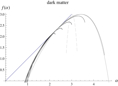
Figure 2: Multifractal spectra at scales $l=2^{-12},2^{-11},\ldots,2^{-7}$, plotted with solid lines in succesively lighter tones of grey. The light dashed lines are the spectra of the homogeneous distributions at $l=2^{-3}$.

Another interesting dimension is $D_{0}$, the box-counting dimension of the distribution’s support. Since it coincides with the maximum of $f(\alpha)$, Fig. 2 shows that a reliable value of $D_{0}$ can only be obtained from the scale $l=2^{-8}$ upwards. This value is 3, confirming the conclusion that the cosmic web is a non-lacunar multifractal [11]. Note that having $D_{0}=3$ implies that the empty cells that appear in increasing numbers for $l\leq 2^{-8}$ are actually empty because they belong to under-sampled zones. Moreover, the high-$\alpha$ ends of the spectra at scales $l<2^{-8}$ are given by scarcely occupied cells and, naturally, deviate from the true spectrum (best represented at $l=2^{-7}$); in particular, the maximum of $f(\alpha)$ is depressed, creating the false impression of lacunarity. In fact, it is necessary to suppress scarcely occupied cells to fully demonstrate scale invariance, as we show next.

3.3 Scaling of second order moments and correlation dimensions

The superposition of the coarse spectra at $l=2^{-12},\ldots,2^{-7}$ in their respective $\alpha$ ranges that is shown in Fig. 2 constitutes a proof of multifractality. However, the standard proof of scale invariance for multifractals is based on the definition of $\tau$-exponents in Eq. (3): scale invariance demands the scaling of $M_{q}$ in a range of cell sizes that is sufficient to calculate a meaningful $\tau(q)$ and, hence, $D_{q}$. The exponent $\tau(q)$ is normally calculated by fitting the slope of the plot of $\log M_{q}$ versus $\log l$. We now follow this procedure.

First of all, we need to select the values of $q$ for which we calculate $M_{q}$ and also select the appropriate range of cell sizes. The available range of $q$ is bound above by the condition that $f(\alpha)\geq 0$ (non-negative fractal dimensions). This bound can be perceived in Fig. 2, for the slopes of the spectra do not become vertical at their left-hand ends, that is to say, the respective values of $q=f^{\prime}(\alpha)$ are bounded above. The bound depends somewhat on the particular spectrum and, in fact, becomes smaller as $l$ grows. An examination of the numerical values of $q$ for the spectra plotted in Fig. 2 reveals that the largest integer value of $q$ that is common to all the spectra is $q=2$. Note that the values of $f^{\prime}(\alpha)$ differ much more than the respective values of $f(\alpha)$.

The possible values of $q$ must also be bounded below: although most spectra in Fig. 2 can be nominally extended to $q=f^{\prime}(\alpha)\rightarrow-\infty$, this extension is inside their unreliable high-$\alpha$ ends. For example, it is obvious from Fig. 2 that the spectrum at $l=2^{-12}$ (for either dark matter or gas) does not represent well the mass concentrate, corresponding to the point of contact with the diagonal. Therefore, that spectrum is not valid even down to $q=1$. Consequently, when we combine the upper and lower bounds, the only integer value allowed is $q=2$, so we must restrict ourselves to examining the scaling of $M_{2}$ and calculating the correlation dimension $D_{2}=\tau(2)$. Notice that this dimension is of special interest, since it is the one that is usually measured in galaxy surveys.

As regards the range of cell sizes in which to look for scaling, the natural range lies between the homogeneity scale $l=2^{-4}$ and the discreteness scale $l=2^{-10}$. However, we have seen above that the effects of under-sampling can already be perceived at $l=2^{-8}$ and become more evident at $l=2^{-9}$. On the other hand, the cells that are well populated on scales $l\leq 2^{-8}$ are surely not affected by under-sampling, as proved by the superposition of the spectra along their left-hand sides. A sensible way to avoid the effects of under-sampling in the computation of $M_{2}$ is to suppress for each $l$ the scarcely occupied cells that contribute to the deviant piece of the corresponding multifractal spectrum. Thus, we set a lower cell-mass cutoff $m=m_{0}(l/l_{0})^{\alpha}$, where $l_{0}=2^{-4}$, $m_{0}=Nl_{0}^{3}=2^{18}$ and, for each $l$, we choose the value of $\alpha$ that marks the beginning of the deviant spectrum. To be definite, we assume that the deviant pieces of the spectra begin at their respective maxima (see Fig. 2). Thus, we can proceed to $l<2^{-10}$, but we stop at $l=2^{-12}$ because lower scales present several problems: (i) the spectrum hardly represents the mass concentrate; (ii) the value of $M_{2}$ becomes very sensitive to the precise value of the $m$-cutoff; (iii) the gas distribution begins to noticeably depart from the dark-matter distribution.

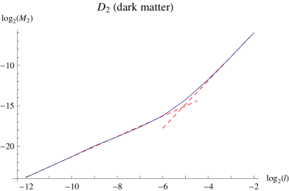
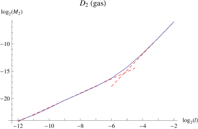
Figure 3: Log-log plots for the correlation dimension $D_{2}$ of the distributions of dark-matter (left) and gas (right), showing the fractal scaling range and the transition to homogeneity.

Therefore, we compute $M_{2}$ from the scale $l=2^{-12}$ upwards, and actually we do not stop at $l=2^{-4}$ but at $l=2^{-2}$, to study the full transition to homogeneity. The log-log plots of $M_{2}$ versus scale $l$ are displayed in Fig. 3. The dashed straight lines correspond to the least-squares fits. The two fits in the fractal ranges between $l=2^{-12}$ and $l=2^{-6}$ yield the following dimensions: (i) $D_{2}=1.255\pm 0.012$ for the dark-matter; (ii) $D_{2}=1.30\pm 0.02$ for the gas. The two fits in the homogeneity ranges yield values of $D_{2}$ very close to three, of course.

In each plot, the scale at which the straight line of the fractal fit meets the straight line of the homogeneity fit is a measure of the scale of transition to homogeneity $l_{0}$. Thus, we deduce that $l_{0}=2^{-5}$, approximately, for both the dark matter and the gas. Notice that this measure of the scale of homogeneity yields a smaller value than the one that we have been using, $l_{0}=2^{-4}$. In fact, the transition to homogeneity is not very sharp but takes place between $l=2^{-6}$ and $l=2^{-4}$, as Fig. 3 shows.

The value $D_{2}=1.30\pm 0.02$ for the gas is definitely smaller than the galaxy correlation dimension $D_{2}=2.0\pm 0.1$ obtained by Sylos Labini and Pietronero [14] but agrees with conventional values of $D_{2}$ [13, 14]. Sylos Labini and Pietronero’s value stems from their criticism of the treatment of finite size effects and, in particular, from questioning the classical value of the scale of homogeneity $r_{0}\simeq 5\,h^{-1}\!$ Mpc. Indeed, they extend the scaling range of the correlation function up to $30\,h^{-1}\!$ Mpc and, consequently, $D_{2}$ grows. Other authors also find $D_{2}\simeq 2$, especially when they use long scale ranges to compute it (see Table I in Ref. [13]). In our case, the end of the scaling range at $l=2^{-6}$ is quite clear, although we define as homogeneity scale $l_{0}=2^{-5}$ (a fit up to this scale would hardly raise $D_{2}$, anyway). The scale $l=2^{-6}$ is $7.8\,h^{-1}\!$ Mpc in physical units.

To summarize the results of Sect. 3, the tests for scale invariance can be considered successful, given the limitations imposed by the data. Of course, the scaling range necessary to affirm scale invariance is a matter of opinion. A factor of $2^{-6}=64$ is reasonably good. In addition to the extent of a scaling range, one must also consider the quality of the corresponding least-squares fit, namely, its standard error. In this regard, the fits for the dark-matter and gas distributions are both remarkably good. We refrain from affirming that we have proved that these distributions are (samples of) statistically self-similar multifractals, but we assert that there is strong evidence of it. Furthermore, there is good evidence that the dark-matter and gas distributions are indistinguishable multifractals. One could object that the confidence intervals for the $D_{2}$ do not overlap and that there are minute differences between the respective plots in Figs. 1 and 2. To assess the statistical significance of the numerical differences between the distributions of dark-matter or gas particles, we carry out next a detailed study.

4 Relation between the gas and dark-matter distributions

We see that the multifractal properties of the dark-matter and gas distributions are very similar (along a considerable range of scales), which suggests that the distributions could actually be identical. In general, one may ask if two finite samples of continuous distributions can come from the same continuous distribution. In particular, it is possible that the differences between the distributions of gas and dark matter particles are only due to statistical sample variance, while the continuous gas distribution is unbiased with respect to the total mass distribution (dominated by the dark matter). We know that the gas dynamics is different from the collisionless dark-matter dynamics, with the likely result of bias, but we need to ascertain the existence of bias from the actual particle distributions by means of statistical tests.

The first test that comes to one’s mind is based on the cross-correlation function of gas and dark-matter particles, in particular, the cross-correlation coefficient, useful to measure the similarity of two distributions. Indeed, this test confirms that both distributions are very similar, as we show in sub-section 4.1. However, this test cannot prove that the samples actually come from the same continuous distribution. In fact, it is easy to see that there is no way to prove it and we must satisfy ourselves with obtaining a probability of its being true. Rather, assuming a Bayesian point of view, we can quantify the “degree of belief” in the hypothesis that there is a common continuous distribution (sub-section 4.2). The application of this method in sub-sect. 4.3 allows us to confidently conclude that the gas distribution is biased on nonlinear scales. Then, we study the nature of that bias in sub-section 4.4.

To compare the two distributions at several scales, we use counts in cells, like in the multifractal analysis. Thus, we assume that two independent continuous distributions define the probabilities of the respective counts in cells of given size. In other words, we assume that the dark-matter and gas distributions are both samples of respective multinomial distributions, each one given by a set of probabilities defined in the cells. The cross-correlation can be easily expressed in terms of counts in cells. The Bayesian method seeks the probability (degree of belief) that two multinomial samples come from the same multinomial distribution 4.2.

4.1 Cross-correlations

Given a mass distribution coarse-grained with volume scale $V$, its auto-correlation is measured by the second order cumulant

$${\bar{\xi}}_{2}=\frac{1}{V^{2}}\int_{V}d^{3}x_{1}\,d^{3}x_{2}\,\xi_{2}(x_{1},x_{2}),$$

where ${\xi}_{2}$ is the two-point correlation function of the fine grain distribution. In the nonlinear regime,

$${\bar{\xi}}_{2}=\frac{\langle\rho^{2}\rangle}{\langle\rho\rangle^{2}}-1\approx\frac{\langle\rho^{2}\rangle}{\langle\rho\rangle^{2}}=\frac{\mu_{2}}{\mu_{1}^{2}}\gg 1.$$

We can define the cross-correlation coefficient of gas (g) and dark-matter (m) at scale $V$ as

$${c}_{\rm gm} = \frac{{\bar{\xi}}_{\rm gm}}{\left(\bar{\xi}_{\rm 2g}\,\bar{\xi}_{\rm 2m}\right)^{1/2}}=\frac{\langle\rho_{\rm g}\,\rho_{\rm m}\rangle}{\left(\langle\rho_{\rm g}^{2}\rangle\,\langle\rho_{\rm m}^{2}\rangle\right)^{1/2}}=\frac{\sum_{i=1}^{M}n_{{\rm g}\,i}\,n_{{\rm m}\,i}}{\left(\sum_{i=1}^{M}n_{{\rm g}\,i}^{2}\right)^{1/2}\left(\sum_{i=1}^{M}n_{{\rm m}\,i}^{2}\right)^{1/2}}\,,$$

where the last expression refers to counts in volume-$V$ cells and $M$ denotes the number of these cells. The cross-correlation coefficient can be viewed as the cosine of the angle formed by the two $M$-dimensional vectors $\{n_{{\rm g}\,i}\}$ and $\{n_{{\rm m}\,i}\}$.

Given the cell counts $\{n_{{\rm g}\,i}\}$ and $\{n_{{\rm m}\,i}\}$, we can compute ${c}_{\rm gm}$ at once, but we follow instead a more elaborate procedure to discern the influence of the cell masses. We first rank the cells in order of decreasing physical mass, for physical mass determines the importance of cells in regard to gravity. Then, we compute the cross-correlation coefficient of the ordered cells up to successive rank values. In Fig. 4, we plot the cross-correlation coefficient of the gas and dark-matter in massive halos (taken from the master cell distribution), computed in that way. This coefficient is stably above 0.99, that is to say, the correlation between both distributions is very strong. Moreover, the cross-correlation coefficient increases with the coarse-graining scale $l$. For example, it reaches 0.9999 at $l=2^{-5}$. However, we have no way of knowing how strong the correlation must be for allowing us to affirm that both samples come from the same distribution.

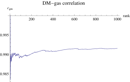
Figure 4: Cross-correlation coefficient of gas and dark matter in massive halos, as a function of the number of halos, ranked in order of decreasing mass.

4.2 Bayesian comparison of multinomial distributions

Bayes’ theory of probability interprets the concept of probability as a measure of a state of knowledge. Bayes’ theorem tells us how to adjust probabilities in regard to new evidence. It writes

$$P(H|E)=\frac{P(E|H)\,P(H)}{P(E)}\,,$$

where $H$ is a hypothesis with prior probability $P(H)$, $E$ is an event that provides new evidence for $H$, and $P(E|H)$ is the conditional probability of having $E$ if the hypothesis $H$ happens to be true. $P(E)$ is the a priori probability of observing the event $E$ under all possible hypotheses. $P(H|E)$ adjusts $P(H)$ and is called the posterior probability of $H$ given $E$. Bayesian analysis is routinely employed for model selection in many scientific areas.

In Bayes’ theorem, the hypothesis $H$ can belong to a continuum of possibilities. For example, if we are given the results of $N$ trials of a binomial experiment, we can analyse the information gained from them on the probability $p$ of “success” (“success” is defined arbitrarily as one of the two possible outcomes). This probability is a number $0<p<1$ (while the probability of “failure” is $1-p$). For a given value of $p$, the probability of $n$ successes in $N$ trials is given by the binomial distribution

$$P(N,n|p)=\binom{N}{n}\,p^{n}(1-p)^{N-n}.$$

Since $N$ and $n$ are given and $p$ is unknown, we can apply Bayes’ theorem in the form

$$P(p|N,n) = \frac{P(N,n|p)\,P(p)}{\int_{0}^{1}P(N,n|p)\,P(p)\,dp}=\frac{p^{n}(1-p)^{N-n}\,P(p)}{\int_{0}^{1}p^{n}(1-p)^{N-n}\,P(p)\,dp}\,.$$

It yields the probability of $p$ given the data in terms of the prior probability of $p$. If no prior information about $p$ is available, we must assume that $P(p)=1$ (according to the principle of insufficient reason). Then, the posterior probability $P(p|N,n)$ is the beta distribution with parameters $n+1$ and $N-n+1$. It is trivial to check that it reaches its maximum at $p=n/N$ (mode value) and that its variance is proportional to $1/N$ (for fixed $n/N$ and large $N$).

This example is, in fact, relevant to our problem, namely, to estimating the probability that the given gas and dark-matter samples belong to the same distribution. If we choose one cell, with $n_{{\rm m}}$ dark-matter particles, say, the probability that the mass fraction in that cell is $p_{{\rm m}}$ is given by the beta distribution with parameters $n_{{\rm m}}+1$ and $N_{{\rm m}}-n_{{\rm m}}+1$ ($N_{{\rm m}}$ being the total number of dark-matter particles in the sample). Analogously, the probability of a gas mass fraction $p_{{\rm g}}$ in that cell is given by the beta distribution with parameters $n_{{\rm g}}+1$ and $N_{{\rm g}}-n_{{\rm g}}+1$. We can obtain the probability of the difference $p_{{\rm m}}-p_{{\rm g}}$ by taking the product $P(p_{{\rm m}}|n_{{\rm m}},N_{{\rm m}})P(p_{{\rm g}}|n_{{\rm g}},N_{{\rm g}})$, performing the change of the variables $p_{{\rm m}}$ and $p_{{\rm g}}$ to $p_{{\rm m}}-p_{{\rm g}}$ and $(p_{{\rm m}}+p_{{\rm g}})/2$, and integrating over the second variable (within the appropriate limits). However, the difference $p_{{\rm m}}-p_{{\rm g}}$ is a continuous variable and its probability is a probability density; therefore, the probability that $p_{{\rm m}}=p_{{\rm g}}$ vanishes. Nevertheless, we expect to get some information from the value of the probability density at $p_{{\rm m}}=p_{{\rm g}}$. Thus, we calculate

$$\int_{0}^{1}P(p|n_{{\rm m}},N_{{\rm m}})\,P(p|n_{{\rm g}},N_{{\rm g}})\,dp=$$ (15)

$$\phantom{aaaaaaaa}\frac{B(n_{{\rm m}}+n_{{\rm g}}+1,N_{{\rm m}}-n_{{\rm m}}+N_{{\rm g}}-n_{{\rm g}}+1)}{B(n_{{\rm m}}+1,N_{{\rm m}}-n_{{\rm m}}+1)\,B(n_{{\rm g}}+1,N_{{\rm g}}-n_{{\rm g}}+1)}\,,$$

where ${B(x,y)=\Gamma(x)\,\Gamma(y)/\Gamma(x+y)}$ is the Euler beta function. The value of the integral is enhanced when the maxima of $P(p|n_{{\rm m}},N_{{\rm m}})$ and $P(p|n_{{\rm g}},N_{{\rm g}})$ coincide, namely, when $n_{{\rm m}}/N_{{\rm m}}=n_{{\rm g}}/N_{{\rm g}}$. For fixed $N_{{\rm m}}=N_{{\rm g}}$, the function on the right-hand side of Eq. (15) is a symmetric function of $\{n_{{\rm m}},n_{{\rm g}}\}$. Therefore, for a fixed value of $n_{{\rm m}}+n_{{\rm g}}$, it is just a symmetric function of the difference $n_{{\rm m}}-n_{{\rm g}}$ and has its maximum when $n_{{\rm m}}=n_{{\rm g}}$.

One could criticize the preceding approach for only focusing on the value of the probability density at $p_{{\rm m}}=p_{{\rm g}}$, while values of $p_{{\rm m}}-p_{{\rm g}}$ close to zero might also be relevant. We can avoid the problem of having to deal with a continuous probability by singling out the value $p_{{\rm m}}=p_{{\rm g}}$ from the outset. Thus, we formulate a Bayesian analysis with this hypothesis and the event $E=\{n_{{\rm m}},N_{{\rm m}},n_{{\rm g}},N_{{\rm g}}\}$:

$$P(p_{{\rm m}}=p_{{\rm g}}|E)=\frac{P(p_{{\rm m}}=p_{{\rm g}})\,P(E|p_{{\rm m}}=p_{{\rm g}})}{P(p_{{\rm m}}=p_{{\rm g}})\,P(E|p_{{\rm m}}=p_{{\rm g}})+P(p_{{\rm m}}\neq p_{{\rm g}})\,P(E|p_{{\rm m}}\neq p_{{\rm g}})}\,.$$

Here, $P(E|p_{{\rm m}}\neq p_{{\rm g}})$ is just the probability of $E$ given any values of $p_{{\rm m}}$ and $p_{{\rm g}}$, because the event $p_{{\rm m}}=p_{{\rm g}}$ has probability zero; namely,

$$P(E|p_{{\rm m}}\neq p_{{\rm g}})=\binom{N_{{\rm m}}}{n_{{\rm m}}}\binom{N_{{\rm g}}}{n_{{\rm g}}}\int_{0}^{1}dp_{{\rm m}}\int_{0}^{1}dp_{{\rm g}}\,p_{{\rm m}}^{n_{{\rm m}}}(1-p_{{\rm m}})^{N_{{\rm m}}-n_{{\rm m}}}\,p_{{\rm g}}^{n_{{\rm g}}}(1-p_{{\rm g}})^{N_{{\rm g}}-n_{{\rm g}}}.$$

On the other hand,

$$P(E|p_{{\rm m}}=p_{{\rm g}}) = \binom{N_{{\rm m}}}{n_{{\rm m}}}\binom{N_{{\rm g}}}{n_{{\rm g}}}\int_{0}^{1}dp\,p^{n_{{\rm m}}+n_{{\rm g}}}(1-p)^{N_{{\rm m}}-n_{{\rm m}}+N_{{\rm g}}-n_{{\rm g}}}.$$

Computing the integrals and substituting, we obtain

$$P(p_{{\rm m}}=p_{{\rm g}}|E)=\frac{P(p_{{\rm m}}=p_{{\rm g}})\,b(n_{{\rm m}},N_{{\rm m}};n_{{\rm g}},N_{{\rm g}})}{P(p_{{\rm m}}=p_{{\rm g}})\,b(n_{{\rm m}},N_{{\rm m}};n_{{\rm g}},N_{{\rm g}})+P(p_{{\rm m}}\neq p_{{\rm g}})\,}\,,$$

where

$$b(n_{{\rm m}},N_{{\rm m}};n_{{\rm g}},N_{{\rm g}}) = \frac{P(E|p_{{\rm m}}=p_{{\rm g}})}{P(E|p_{{\rm m}}\neq p_{{\rm g}})}$$ (16)

$$= \frac{B(n_{{\rm m}}+n_{{\rm g}}+1,N_{{\rm m}}-n_{{\rm m}}+N_{{\rm g}}-n_{{\rm g}}+1)}{B(n_{{\rm m}}+1,N_{{\rm m}}-n_{{\rm m}}+1)\,B(n_{{\rm g}}+1,N_{{\rm g}}-n_{{\rm g}}+1)}\,.$$ (17)

This function of $\{n_{{\rm m}},N_{{\rm m}},n_{{\rm g}},N_{{\rm g}}\}$ coincides with the value of the probability density of $p_{{\rm m}}-p_{{\rm g}}$ at 0 given by Eq. (15). Therefore, this approach is consistent with the preceding one: if $b(n_{{\rm m}},N_{{\rm m}};n_{{\rm g}},N_{{\rm g}})$ is large, then $P(p_{{\rm m}}=p_{{\rm g}}|E)$ tends to one, independently of the prior probability $P(p_{{\rm m}}=p_{{\rm g}})$. However, we have no way of estimating this prior probability.

The assignment of prior probabilities is a usual problem in Bayesian analyses, to the extent that Bayes’ theory of probability has been deemed subjective. However, there is no subjectivity if we indeed understand Bayes’ theory as a way of adjusting probabilities in regard to new evidence. The Bayes factor defined in Eq. (16) is such that

$$\log\frac{P(p_{{\rm m}}=p_{{\rm g}}|E)}{P(p_{{\rm m}}\neq p_{{\rm g}}|E)}=\log b(n_{{\rm m}},N_{{\rm m}};n_{{\rm g}},N_{{\rm g}})+\log\frac{P(p_{{\rm m}}=p_{{\rm g}})}{P(p_{{\rm m}}\neq p_{{\rm g}})}\,.$$

Hence, we can endow this equation with an information theory meaning: the prior information about the odds of our hypothesis is updated by the information $\log b$ provided by the event $E=\{n_{{\rm m}},N_{{\rm m}},n_{{\rm g}},N_{{\rm g}}\}$. The prior information is null if $P(p_{{\rm m}}=p_{{\rm g}})=P(p_{{\rm m}}\neq p_{{\rm g}})$, but the information provided by the event is independent of any prior probabilities. The information provided by $E$ is positive or negative according to whether the Bayes factor is larger or smaller than one. The addition of informations is independent of the (common) base of the logarithms, but it is convenient to use base two and measure the information in bits. If the Bayes factor is larger than one half and smaller than two, the information provided by $E$ is smaller than one bit and can hardly be considered significant. For example, with $N_{{\rm m}}=N_{{\rm g}}=200$, $\log_{2}b(100,200;100,200)=3.00$ bits, $\log_{2}b(100,200;80,200)=0.11$ bits, and $\log_{2}b(100,200;70,200)=-3.61$ bits, and only the first case or the last case provide evidence for or against $p_{{\rm m}}=p_{{\rm g}}$, respectively.

Since we actually divide the sample into many cells, we need to generalize the above method of comparing binomial distributions to the case of multinomial distributions. This generalization is straightforward, except that we now have to take care of normalizing the $P(E|\cdot)$ such that $\sum_{E}P(E|\cdot)=1$. The resulting Bayes factor is

$$b(n_{{\rm m}\,1},\ldots,n_{{\rm m}\,k};n_{{\rm g}\,1},\ldots,n_{{\rm g}\,k})=$$

$$\phantom{aaaaaaaa}\frac{B(n_{{\rm m}\,1}+n_{{\rm g}\,1}+1,\ldots,n_{{\rm m}\,k}+n_{{\rm g}\,k}+1)}{B(n_{{\rm m}\,1}+1,\ldots,n_{{\rm m}\,k}+1)\,B(n_{{\rm g}\,1}+1,\ldots,n_{{\rm g}\,k}+1)\,(k-1)!}\,,$$

where $\{n_{{\rm m}\,i}\}_{i=1}^{k}$ and $\{n_{{\rm g}\,i}\}_{i=1}^{k}$ are the vectors denoting the numbers of dark-matter and gas particles, respectively, in the $k$ cells, and $B(x_{1},\ldots,x_{k})=\Gamma(x_{1})\cdots\Gamma(x_{k})/\Gamma(x_{1}+\cdots+x_{k})$ is the generalized Euler beta function. We can write this Bayes factor as follows:

$$b(n_{{\rm m}\,1},\ldots,n_{{\rm m}\,k};n_{{\rm g}\,1},\ldots,n_{{\rm g}\,k})=$$ (18)

$$\phantom{aaaaaaaaaaa}\binom{n_{{\rm m}\,1}+n_{{\rm g}\,1}}{n_{{\rm m}\,1}}\cdots\binom{n_{{\rm m}\,k}+n_{{\rm g}\,k}}{n_{{\rm m}\,k}}\frac{(N_{{\rm m}}+k-1)!\,(N_{{\rm g}}+k-1)!}{(N_{{\rm m}}+N_{{\rm g}}+k-1)!\,(k-1)!}\,,$$

where $N_{{\rm m}}=n_{{\rm m}\,1}+\cdots+n_{{\rm m}\,k}$ and $N_{{\rm g}}=n_{{\rm g}\,1}+\cdots+n_{{\rm g}\,k}$ are the total numbers of dark-matter and gas particles, respectively (which are equal, in our case). The latter form has the advantage of being the product of $k$ binomial numbers, one per cell, times an overall factor. Each binomial number expresses the number of ways of dividing the total number of particles in the corresponding cell between the respective numbers of gas and dark-matter particles. We can associate the (base-two) logarithm of that binomial number with a “cell entropy”. This entropy is maximal when the numbers of dark-matter and gas particles in the cell are equal and vanishes when there are no particles of one type in the cell.

Let us take $N_{{\rm m}}=N_{{\rm g}}=N$. To compute the Bayes factor, we follow an analogous procedure to the one employed to compute the cross-correlation coefficient ${c}_{\rm gm}$. Since the above-described Bayesian analysis is valid for any multinomial distribution or, in other words, the cells are of logical rather than physical nature, we can group several physical cells into one. In particular, we can group the less significant cells, namely, the ones with small numbers of particles. A systematic procedure for grouping the cells consists in ordering them by decreasing total number of particles and separating the most populated ones to take them first into account. Thus, we take the first rank cell and compare it against the remainder, using the binomial Bayes factor. The evidence for or against $p_{{\rm m}}=p_{{\rm g}}$ cannot be considered definitive yet. Then, we proceed to calculate the Bayes information of the two more populated cells plus the “cell” with the remainder, and so onwards. If a definite trend is soon established, that is to say, if the absolute value of the Bayes information grows steadily, we consider it as a solid evidence for or against the hypothesis, according to the sign of $\log_{2}b$.

4.3 Bayesian analysis of the distributions at several scales

Here, we apply the above-explained procedure of systematic multinomial Bayesian analysis to some relevant cell distributions. We prefer to rank the cells again in order of decreasing physical mass, as in Sect. 4.1, rather than in order of decreasing total number of particles.

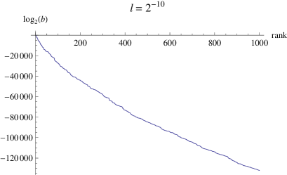
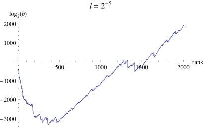
Figure 5: Bayesian evidence (in bits) for the equality of distributions ($p_{{\rm m}}=p_{{\rm g}}$) derived from massive cells at $l=2^{-10}$ (halos) and at $l=2^{-5}$ (transition to homogeneity).

We calculate the Bayes information $\log_{2}b$ (in bits) for the hypothesis $p_{{\rm m}}=p_{{\rm g}}$, considering a growing number of the most massive cells. The result is plotted in Fig. 5, for the two most relevant scales: $l=N^{-1/3}=2^{-10}$ (corresponding to the master cell distributions) and $l=2^{-5}$ (the scale of transition to homogeneity). In the first case, we see that the 1000 most massive halos already show that the evidence against the hypothesis is overwhelming: note that $\log_{2}b$ reaches $-130$ Kbits and keeps its downward tendency. The evidence in the second case is mixed: it is increasingly negative up to the 500th rank, reaching $-3$ Kbits, but there it starts growing and becomes positive from the 1550th rank onwards (the 1550th cell contains $84\hskip 1.0pt678$ dark matter particles and $83\hskip 1.0pt885$ gas particles). Considering that the total number of cells is $l^{-3}=2^{15}=32\hskip 1.0pt768$ and that the corresponding total Bayes information is 185.4 Kbits, we could say that the evidence of the hypothesis $p_{{\rm m}}=p_{{\rm g}}$ is sufficient. However, the most massive cells clearly distinguish both distributions.

Proceeding to larger scales, namely, to $l=2^{-4}$, the above pattern holds. At $l=2^{-4}$, the Bayes information has some small fluctuations about zero in the first ranks, staying above $-97$ bits, and then it definitely grows, reaching a total of 28.8 Kbits. In this case, the evidence for $p_{{\rm m}}=p_{{\rm g}}$ is solid. Of course, the evidence for $p_{{\rm m}}=p_{{\rm g}}$ is stronger at larger $l$.

Regarding the origin of the difference between $p_{{\rm m}}$ and $p_{{\rm g}}$ on small scales, let us focus on the master cell distributions. An inspection of the dark-matter and gas particle counts in massive halos reveals that these consistently have fewer gas particles than dark-matter particles. The smaller average number of gas particles is clearly observed in the respective log-log plots of counts in cells ranked by total physical mass, which are shown in Fig. 6. We observe in the figure that both distributions approximately follow linear log-log laws (sort of Zipf’s laws), with common slope, but the line that corresponds to the dark-matter particles is definitely above. In other words, the massive halos concentrate less gas, although the number of gas particles decreases according to the same pattern that the number of dark-matter particles. One can also notice that there are more fluctuations in the number of gas particles, due to their smaller physical mass.

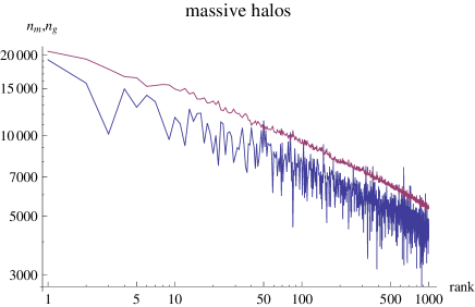
Figure 6: Particle counts of dark-matter (upper line) and gas (lower line) in halos ranked in order of decreasing mass.

It is useful to express the differences between dark-matter and gas particle counts in terms of the cell entropies introduced in Sect. 4.2 after Eq. (18), as we do next.

4.4 Entropic difference between the gas and dark-matter distributions

In the expression (18) of the Bayes factor, we can consider that the $k$ cells consist of a small number of massive cells $h=k-1$ (in order of decreasing mass) and a $k$-th “cell” containing the remaining particles. Furthermore, we assume that the $h$ massive cells contain together a total number of particles that is small in comparison with the total number of particles. Recalling that $N_{{\rm m}}=N_{{\rm g}}=N=2^{30}\gg 1$, we can make a suitable approximation of the Bayes information $\log_{2}b$. Indeed, under the given conditions, the largest contributions to the Bayes information come from the cell with the remaining particles and from the overall factor in Eq. (18); namely,

$$\log_{2}\binom{2N-\sum_{i=1}^{h}(n_{{\rm m}\,i}+n_{{\rm g}\,i})}{N-\sum_{i=1}^{h}n_{{\rm g}\,i}}=2N-\sum_{i=1}^{h}(n_{{\rm m}\,i}+n_{{\rm g}\,i})-\frac{\log_{2}(\pi N)}{2}+{\mathop{\rm O}\nolimits(N^{-1})}$$

and

$$\log_{2}\frac{(N+h)!\,^{2}}{(2N+h)!\,h!}=-2N+h\,\log_{2}\frac{N}{2}+\frac{\log_{2}(\pi N)}{2}+{\mathop{\rm O}\nolimits(N^{-1})}-\log_{2}h!\,,$$

where we have used Stirling’s approximation. Note that both contributions have a first term proportional to $N$, but these large terms cancel one another. Therefore,

$$\log_{2}b = \sum_{i=1}^{h}\left[\log_{2}\binom{n_{{\rm m}\,i}+n_{{\rm g}\,i}}{n_{{\rm g}\,i}}-(n_{{\rm m}\,i}+n_{{\rm g}\,i})\right]+$$ (19)

$$h\,\log_{2}\frac{N}{2}-\log_{2}h!+{\mathop{\rm O}\nolimits(N^{-1})}\,,$$

which only grows logarithmically with $N$. This Bayes information is a sum of individual cell contributions plus a global contribution. Each cell contribution is negative, because the cell entropy is bounded above by the number of particles in the cell, as is easily proved. If each massive cell contribution is larger in absolute value than $\log_{2}(N/2)=29$ bits, on average, the total information due to the $h$ massive cells plus the remainder is negative.

In particular, each massive halo contributes, on average, more than $\log_{2}(N/2)=29$ bits (in absolute value). This is the reason why the total Bayes information of a considerable number of massive halos is negative (as shown in Fig. 5). For example, the contribution of the most massive halo, with $n_{{\rm g}}=19\hskip 1.0pt200$ and $n_{{\rm m}}=20\hskip 1.0pt658$, is $\log_{2}\binom{39\hskip 1.0pt858}{19\hskip 1.0pt200}-39\hskip 1.0pt858=-38.5$ bits, larger in absolute value than 29 bits.

The contribution of a massive cell to the Bayes information can be expressed in a more familiar form by using again Stirling’s approximation. When $n_{{\rm m}},n_{{\rm g}}\gg 1$, the cell entropy can be written as

$$\log_{2}\binom{n_{{\rm m}}+n_{{\rm g}}}{n_{{\rm g}}} \approx (n_{{\rm m}}+n_{{\rm g}})\log_{2}(n_{{\rm m}}+n_{{\rm g}})-{n_{{\rm g}}}\log_{2}{n_{{\rm g}}}-{n_{{\rm m}}}\log_{2}{n_{{\rm m}}}$$ (20)

$$= -(n_{{\rm m}}+n_{{\rm g}})\left[{x_{{\rm g}}}\log_{2}{x_{{\rm g}}}+(1-{x_{{\rm g}}})\log_{2}(1-{x_{{\rm g}}})\right],$$ (21)

where we have introduced the fraction of gas particles

$${x_{{\rm g}}}=\frac{n_{{\rm g}}}{n_{{\rm m}}+n_{{\rm g}}}\,$$

(the cell entropy has an analogous expression in terms of the fraction of dark-matter particles). In those forms, the cell entropy can be identified with the familiar entropy of mixing [23]. Given $x_{{\rm g}}$, the cell entropy of mixing is proportional to the total number of particles in the cell; and so is the cell’s contribution to the Bayes information, the proportionality constant being the entropy of mixing per particle minus one. The maximum entropy of mixing per particle is one bit and it corresponds to the most mixed distribution, with $x_{{\rm g}}=1/2$. Naturally, a fully mixed cell makes a vanishing contribution to the Bayes information.

Regarding the master cell distributions, we observe in Fig. 6 that the ratio $n_{{\rm g}\,i}/n_{{\rm m}\,i}$ for massive halos is almost constant on average; in fact, $n_{{\rm g}\,i}/n_{{\rm m}\,i}\simeq 0.81$. Hence, $x_{{\rm g}\,i}\simeq 0.45$, and the entropy of mixing per particle is almost constant and equal to

$$-{x_{{\rm g}}}\log_{2}{x_{{\rm g}}}-(1-{x_{{\rm g}}})\log_{2}(1-{x_{{\rm g}}})\simeq 0.992.$$

Therefore, each halo contribution is roughly proportional to the total number of particles in it, with a common proportionality constant, namely, $0.992-1=-0.008$. This yields about $-250$ bits for the contribution per halo in Eq. (19). Thus, the absolute value of every massive halo contribution is larger than 29 bits, making the total Bayes information in Eq. (19) negative and regularly decreasing with the number of halos, as displayed in Fig. 5 (left). However, the value of the entropy per particle is very close to one, telling us that the distributions are very mixed, even though not completely mixed.

Note that a constant ratio $n_{{\rm g}\,i}/n_{{\rm m}\,i}$ for all the cells would be in contradiction with $N_{{\rm g}}=N_{{\rm m}}$. Thus, the ratio $n_{{\rm g}\,i}/n_{{\rm m}\,i}\simeq 0.81$, for example, must grow eventually, as $i$ runs over scarcely occupied cells. Even assuming that the ratio $n_{{\rm g}\,i}/n_{{\rm m}\,i}$ stays almost constant as the cell mass diminishes, the contribution per cell to the Bayes information is proportional to the total number of particles in it and, therefore, it must eventually become smaller than 29 bits (in absolute value). For one reason or another, the initial downward trend of the Bayes information must cease and turn upwards. This turn is observed in the plot for $l=2^{-5}$ in Fig. 5.

4.4.1 Connection with thermodynamics

In thermodynamics, the entropy of mixing is, of course, only one part of the total entropy. When other thermodynamic parameters are equal, the entropy of mixing determines the equilibrium configuration to be the most mixed distribution. In our context, the gas and the dark matter are not comparable thermodynamically because, in principle, cold dark matter does not have temperature or pressure. However, CDM particles have velocity dispersion, such that one can assign it a temperature and, hence, a thermodynamic entropy (independent of the properties of the gas). This is the dark-matter entropy considered by Faltenbacher et al [4] in their study of the entropy of gas and dark-matter clusters from the Mare-Nostrum universe. Once the dark matter is assigned thermal states, it is legitimate to compare them with the thermal states of the gas.

In a mixture of ideal gases, the chemical potential of each gas can be expressed as

$$\mu=-T\log_{2}\frac{\zeta(T)}{n}$$

[23], where $n$ is the number density, $\zeta(T)$ is an increasing function of $T$ characteristic of each gas, and we use units consistent with measuring the entropy in bits. The function $\zeta(T)$ is calculated from the possible states of the gas particles (translational and internal states); for a monoatomic gas, $\zeta(T)\propto T^{3/2}$. The condition of “chemical” equilibrium of gas and dark matter is

$$\frac{\mu_{{\rm g}}}{T_{{\rm g}}}=\frac{\mu_{{\rm m}}}{T_{{\rm m}}}\,,$$

which allows for ${T_{{\rm g}}}\neq{T_{{\rm m}}}$. In fact, chemical equilibrium implies

$$\frac{\zeta_{{\rm g}}(T)}{n_{{\rm g}}}=\frac{\zeta_{{\rm m}}(T)}{n_{{\rm m}}}\,\Rightarrow\,\frac{\zeta_{{\rm g}}(T)}{\zeta_{{\rm m}}(T)}=\frac{n_{{\rm g}}}{n_{{\rm m}}},$$

and therefore different temperatures for different densities. We have seen above that ${n_{{\rm g}}}/{n_{{\rm m}}}\simeq 0.81$ for massive halos. Hence, assuming that both $\zeta_{{\rm g}}$ and $\zeta_{{\rm m}}$ correspond to monoatomic gases, we deduce that $T_{{\rm g}}/T_{{\rm m}}\simeq 0.87$.

The conclusion that the dark matter temperature is higher than the gas temperature in massive halos may seem counterintuitive. But note that it relies on the assumption of independent local thermodynamical equilibria of dark matter and gas at different but well-defined temperatures, with the local temperature of dark matter given by its local velocity dispersion. This assumption should imply that the dark matter also has pressure and, therefore, its dynamics should be governed by similar equations to the ones that govern the gas dynamics. However, the effects of dark-matter pressure are not considered in the Mare-Nostrum or other $N$-body cosmological simulations.

5 Entropic comparison of distributions

In the comparison of the gas and dark-matter distributions, we have found it useful to introduce a cell entropy, recognizable as the entropy of mixing. In general, the Boltzmann-Gibbs-Shannon (BGS) entropy of a discrete probability distribution $\{p_{i}\}_{i=1}^{M}$ is defined as

$$S(\{p_{i}\})=-\sum_{i=1}^{M}p_{i}\log_{2}p_{i}\,,$$ (22)

and it represents the uncertainty or lack of information of the result of an experiment with that probability distribution. Note that we are using now “discrete” in the normal sense of the word in probability theory, namely, meaning that there is a list of possible events, as opposed to the continuum of possible events in a continuous distribution; but the probabilities $p_{i}$ are continuous variables. The entropy has some desirable properties, such as the bounds $0\leq S(\{p_{i}\})\leq\log_{2}M$, and the property of additivity, in particular, additivity for independent sets of events [24]. This property and the bounds are shared by a uni-parametric class of functions, the Rényi entropies

$$S_{q}(\{p_{i}\})=\frac{\log_{2}(\sum_{i=1}^{M}{p_{i}}^{q})}{1-q},\quad q\neq 1\,.$$ (23)

The value of $S_{1}$ is obtained as the limit $q\to 1$ and it coincides with the standard BGS entropy defined by Eq. (22).

We can apply the definition of entropy to a discrete distribution of $N$ particles in $M$ cells, with occupation numbers $\{n_{i}\}_{i=1}^{M}$ (counts in cells) and hence expected probability distribution $\{p_{i}=n_{i}/N\}_{i=1}^{M}$. The entropy measures the uncertainty of the cell in which an arbitrary particle is located (or a group of $q$ particles, in the case of $S_{q}$ with $q\in\mathbb{N}$). In particular, we can interpret Eq. (22) as follows. According to Boltzmann, one should weight a macroscopical state, given by a set of occupation numbers, with the number of microscopical states compatible with it (the Boltzmann weight). Then, the entropy is the logarithm of this weight. Since the number of states compatible with the occupation numbers $\{n_{i}\}_{i=1}^{M}$ is given by the corresponding multinomial number, the entropy is given by the logarithm of that multinomial number, namely,

$$\log_{2}\binom{N}{n_{1}\cdots n_{M}}\approx-N\sum_{i=1}^{M}p_{i}\log_{2}p_{i}\,,$$

where we have assumed that $n_{i}\gg 1$, equivalent to neglecting the effect of particle discreteness. The entropy per particle $S(\{p_{i}\})$ is positive and bounded above by $\log_{2}M$. If the distribution is uniform, the bound is reached; in particular, the bound is $\log_{2}M=-\log_{2}V$. Then, the distribution contains the largest uncertainty or, equivalently, the smallest information. Moreover, all the Rényi entropies reach the same bound.

Naturally, it is important to know the behaviour of the entropies in the continuum limit of the discrete distribution $\{p_{i}\}_{i=1}^{M}$, as the cell size $V\to 0$ and $M\rightarrow\infty$ (for the distribution of $N$ particles in $M$ cells, one must let $N\rightarrow\infty$ before $M\rightarrow\infty$). Not surprisingly, the entropies diverge in the continuum limit: one needs an infinite amount of information to locate a point in a continuum. Rényi [24] describes the growth of the $S_{q}$ as the distribution becomes continuous in terms of dimensions; namely, he defines for the continuous distribution the dimensions

$$D_{q}=\lim_{V\to 0}\frac{3\,S_{q}(\{p_{i}\})}{-\log_{2}V},$$

assuming that the limit exits. These Rényi dimensions are standard in multifractal analysis; they have been already introduced in Sect. 2, Eq. (7), and used in subsequent sections. The most important Rényi dimension is $D_{1}$, which is defined by the divergence of the standard BGS entropy and is the dimension of the set of singularities where the probability concentrates. Since the full set of Rényi dimensions characterizes the information content of the distribution in the continuum limit, we deduce that all the continuous distributions with the same spectrum of Rényi dimensions appear equivalent in regard to their information content. In particular, every continuous distribution with $D_{q}=3,\;q\in\mathbb{R},$ appears equivalent to a homogeneous and uniform distribution, in which the Rényi entropies reach their upper bound (note that $D_{q}=3$ is the upper bound to the Rényi dimensions). Indeed, only part of the information contained in a continuous distribution is preserved in its Rényi dimensions.

One can further define the information content of a continuous distribution in terms of its probability density [24], if this density is well defined. However, we are studying distributions with singularities. In a singular distribution, the singularities must be confined to a set of zero volume, but they can be crucial for determining the distribution (for example, consider a distribution concentrated in just one point, namely, a Dirac delta distribution). Therefore, let us focus, for the moment, on regular distributions with well-defined probability density $p(x)$ everywhere and $D_{q}=3$ for all $q$. The probability in an element of volume $V$ is given, as $V\to 0$, by $p(x)V$, where $x$ belongs to that element of volume (this dependence of probability on volume derives from the local dimension being $\alpha=3$ everywhere). Therefore,

$$S(\{p_{i}\}) \approx -\sum_{i}p(x_{i})\,V\log_{2}[p(x_{i})\,V]$$

$$= -\sum_{i}p(x_{i})\,V\log_{2}[p(x_{i})]-\log_{2}V,$$

where the sum runs over a partition of the total volume in volume-$V$ elements (a partition in cells, for example). In the limit $V\to 0$, we can write the entropy as the sum of a finite part and a divergent part, namely,

$$S[p(x)]\approx-\int p(x)\,d^{3}x\,\log_{2}[p(x)]-\log_{2}V.$$

Naturally, the divergent part just tells us that $D_{1}=3$, whereas the finite part is a non-trivial integral of the density.

The finite part of the total entropy is not defined in an absolute way: for partitions in unequal volume elements, when the continuum limit is taken, the logarithm in the integrand is replaced with $\log_{2}[\phi(x)p(x)]$, where $\phi(x)$ is a positive function. On the other hand, while the total entropy is always positive, its finite part can be negative. For these reasons, it is necessary to introduce the relative entropy. Conventionally, the entropy of the density $p(x)$ relative to the density $q(x)$ is defined as

$$S(p|q)=\int p(x)\,d^{3}x\,\log_{2}\frac{p(x)}{q(x)}\,,$$

where it is understood that $p(x)=0$ wherever $q(x)=0$. The relative entropy is always positive. It is also called the Kullback or Kullback-Leibler divergence, and it is studied in detail by Kullback [26] (note that “divergence” means discrimination measure in the statistical context). Therefore, the absolute entropy of a coarse-grained distribution gives rise, in the continuum limit, to an absolute part, the dimension, and a relative part, the relative entropy. Only the latter differentiates regular distributions. Notice that the entropy relative to the uniform distribution is simplest but is only defined for distributions over a finite volume (in our case, the unit cube).

These results hold for singular multifractal distributions with $D_{1}<3$, after the necessary adaptations. One singular distribution $\nu$ can be relatively regular, that is to say, it can be regular with respect to another singular distribution $\mu$. This essentially means that the singularities of $\nu$ form a subset of the singularities of $\mu$. The entropy of $\nu$ relative to $\mu$ is defined as

$$S(\nu|\mu)=\int d\nu(x)\,\log_{2}\frac{d\nu(x)}{d\mu(x)}\geq 0,$$

where $d\nu(x)/d\mu(x)$ is the density of $\nu$ with respect to $\mu$ at the point $x$. This relative entropy differentiates one multifractal distribution ($\nu$) from another ($\mu$), when the former is regular with respect to the latter and, in particular, they have the same dimension $D_{1}$. In fact, $S(\nu|\mu)=0$ if and only if $\nu=\mu$.

The Rényi entropy $S_{q}$ (23) also gives rise in the continuum limit to a divergent part, and hence the dimension $D_{q}$, and to a finite part. This finite part motivates the definition of the relative Rényi entropy

$$S_{q}(\nu|\mu)=\frac{1}{1-q}\,\log_{2}\left[\int d\nu(x)\left(\frac{d\nu(x)}{d\mu(x)}\right)^{q-1}\right],\quad q\neq 1\,.$$

However, this relative entropy is less useful than the standard (Kullback-Leibler) relative entropy.

The relative entropy differentiates distributions but has two shortcomings. First, $S(\nu|\mu)$ is only defined when $\nu$ is $\mu$-regular. Second, the relative entropy does not have the necessary properties to qualify as a distance between distributions: it fails to be symmetric or to fulfill the triangle inequality. However, it is possible to define a real distance between any two distributions in terms of their entropies. For discrete distributions, Endres & Schindelin [28] define

$$D^{2}_{PQ} = 2S(R)-S(P)-S(Q)$$

$$= \sum_{i=1}^{M}\left(p_{i}\log_{2}\frac{2p_{i}}{p_{i}+q_{i}}+q_{i}\log_{2}\frac{2q_{i}}{p_{i}+q_{i}}\right),$$

where $P=\{p_{i}\}$, $Q=\{q_{i}\}$ and $R=\{(p_{i}+q_{i})/2\}$. Then, they prove that $D_{PQ}$ is a distance. Furthermore, Endres & Schindelin [28] note that it can be applied to continuous distributions. This follows from the alternative expression

$$D^{2}_{PQ}=S(P|R)+S(Q|R),$$

that is to say, from $D^{2}_{PQ}$ being a sum of relative entropies, in addition to the fact that any two continuous distributions are both regular with respect to their mean. Therefore, $D_{PQ}$ is well defined in the continuum limit of $P$ and $Q$.

Thus, we can measure the distance between the coarse-grained distributions $p_{i}=n_{{\rm g}\,i}/N$ and $q_{i}=n_{{\rm m}\,i}/N$, where $n_{{\rm g}\,i},n_{{\rm m}\,i}\gg 1$, and then we can take the continuum limit. The distribution $R$ corresponds to the total particle distribution. The squared distance between the coarse distributions is

$$D^{2}_{PQ}=2+\frac{1}{N}\sum_{i=1}^{M}\left({n_{{\rm g}\,i}}\log_{2}{n_{{\rm g}\,i}}+{n_{{\rm m}\,i}}\log_{2}{n_{{\rm m}\,i}}-(n_{{\rm m}\,i}+n_{{\rm g}\,i})\log_{2}(n_{{\rm m}\,i}+n_{{\rm g}\,i})\right)$$ (24)

$$=\frac{1}{N}\sum_{i=1}^{M}\left({n_{{\rm g}\,i}}\log_{2}{n_{{\rm g}\,i}}+{n_{{\rm m}\,i}}\log_{2}{n_{{\rm m}\,i}}+(n_{{\rm m}\,i}+n_{{\rm g}\,i})[1-\log_{2}(n_{{\rm m}\,i}+n_{{\rm g}\,i})]\right).$$ (25)

Referring to the expression (20) of the cell entropy, we deduce that, in the sum of terms (one per cell) given by Eq. (25), each term represents the gap between the maximum cell entropy of mixing (one bit per particle) and its actual value, just like in the sum of cell contributions in the Bayes information (19). Naturally, $D^{2}_{PQ}$ decreases with mixing and vanishes for the most mixed distribution $P=Q=R$. Conversely, it takes its maximum, $D^{2}_{PQ}=2$, when $\{n_{{\rm g}\,i}\}$ and $\{n_{{\rm m}\,i}\}$ are disjoint, namely, when they are not mixed at all [as we deduce from Eq. (24)]. Regarding the continuum limits of $P$ and $Q$, Endres & Schindelin’s distance is maximal if they are mutually singular, namely, if they concentrate in disjoint sets. The continuum limits of disjoint $\{n_{{\rm g}\,i}\}$ and $\{n_{{\rm m}\,i}\}$ give rise to two mutually singular distributions but the definition encompasses more general cases.

Let us notice that the above defined statistical distance is consistent with our Bayesian analysis but cannot replace it. Firstly, it relies on the approximation $n_{{\rm g}\,i},n_{{\rm m}\,i}\gg 1$, that is to say, on neglecting the discreteness effect due to particle counts. In this approximation, the entropy of mixing in the form given by Eq. (20) is just the asymptotic form of the cell entropies in Eq. (19); but note that the global contribution in Eq. (19) diverges as $N\rightarrow\infty$. Lastly, it is a general fact that a statistical distance cannot provide a sharp criterion to decide if two discrete distributions are samples from the same continuous distribution, and it is on the same footing as the cross-correlation coefficient in that regard.

Endres & Schindelin’s distance can be connected with a standard statistical measure of discrimination as follows. Let us note that $D^{2}_{PQ}$ adopts a simplified form when $P$ and $Q$ are close [28], namely,

$$D^{2}_{PQ}\approx\frac{1}{\ln 2}\sum_{i=1}^{M}\frac{(p_{i}-q_{i})^{2}}{2(p_{i}+q_{i})}=\frac{1}{2\ln 2}\,\chi^{2}_{PQ}\,,$$

where the last expression refers to Pearson’s chi-square test of discrimination, which can be considered a particular case of the Endres-Schindelin distance. In our case,

$$\chi^{2}=\sum_{i=1}^{M}\frac{(n_{{\rm m}\,i}-n_{{\rm g}\,i})^{2}}{n_{{\rm m}\,i}+n_{{\rm g}\,i}}\,.$$

The chi-square test has the advantage of highlighting that the expected fluctuations of $|n_{{\rm m}\,i}-n_{{\rm g}\,i}|$ in a common distribution are of the order of $(n_{{\rm m}\,i}+n_{{\rm g}\,i})^{1/2}$. At any rate, the test is based on an approximation of $D^{2}_{PQ}$ and neither can it provide a sharp criterion of discrimination.

5.1 Bias as entropic distance

In cosmology, the bulk of mass belongs to the dark matter, so the distribution of gas (or galaxies) is assumed to be “biased” with respect to the total matter distribution, dominated by the dark matter. Since we normalize to one both the dark matter and the gas total masses, both components play a symmetrical rôle in our statistical analyses. Therefore, our measure of bias must be just a measure of discrimination between two probability distributions (a “divergence” or distance). There are many such measures, but the notions of relative entropy and Endres-Schindelin distance naturally arise in connection with our Bayesian analysis. Regarding the Endres-Schindelin distance, mutually singular distributions are most distant, namely, at distance $\sqrt{2}$. This distance diminishes if the distributions concentrate in a common set, but vanishes only when they coincide. The relative entropy is not a distance but it is useful as well, because it diverges for mutually singular distributions and, therefore, it separates distributions better. In fact, the relative entropy can be symmetrized with respect to the compared distributions, and then it diverges unless they are mutually regular.

The simplest example of comparison of two distributions occurs when they are both regular, in particular, when they have everywhere well-defined densities $p(x)$ and $q(x)$. In spite of their individual regularity, they are mutually singular if they do not overlap, that is to say, if each density is positive only where the other density vanishes, then being at Endres-Schindelin distance $\sqrt{2}$. As they overlap more and, furthermore, the densities approach one another, their Endres-Schindelin distance and their symmetric relative entropy tend both to zero. On the other hand, the symmetric relative entropy is finite only if both distributions vanish in the same point set (disregarding sets of zero volume, of course).

Regarding singular distributions, the first condition for two distributions to be at small Endres-Schindelin distance is that they have the same Rényi dimensions and, therefore, the same multifractal spectrum. However, this condition is far from being sufficient. Indeed, the multifractal spectrum only gives the “size” (the dimension) of every set of singularities with common strength (local dimension), but tells us nothing about the precise geometry (location or shape) of those sets. Like in the case of regular distributions, two distributions are at small Endres & Schindelin’s distance if the strength and location of their mass concentrations, in particular, their singularities, essentially coincide. As regards the symmetric relative entropy, the singularities must actually coincide for it to be finite.

It has been remarked above that a statistical distance (or divergence) cannot provide a sharp distinguishability criterion. In fact, the distinguishability criterion provided by the Bayes factor only makes sense for finite point distributions, namely, for deciding if two finite point distributions can be samples from the same multinomial distribution. In this regard, the Bayesian comparison of the dark-matter and gas cell distributions in Sect. 4.3 has clearly ruled out a common multinomial distribution on nonlinear scales. Nevertheless, the entropy of mixing per particle is very close to the maximum of one bit; for example, it is $0.992$ bits for massive halos in the master cell distributions. Therefore, the two distributions are indeed very mixed (very close).

Furthermore, the closeness of the gas and dark matter distributions suggests that their individual singularities coincide and, therefore, the two distributions are mutually regular. In the coarse formalism that we use, the local dimension of cell $i$ is

$$\alpha_{i}=3\frac{\log[n_{i}/(NV_{0})]}{\log(V/V_{0})}\,.$$

Therefore, the difference between the strenghs of gas and dark matter singularities is

$$\alpha_{{\rm g}\,i}-\alpha_{{\rm m}\,i}=3\frac{\log(n_{{\rm g}\,i}/n_{{\rm m}\,i})}{\log(V/V_{0})}\,.$$

We can see that this difference vanishes if $n_{{\rm g}\,i}/n_{{\rm m}\,i}$ stays bounded (above and below) while the cell volume $V$ shrinks. Although we have found that the ratio $n_{{\rm g}\,i}/n_{{\rm m}\,i}$ is not unity in populated cells, its logarithm is small (in absolute value) with respect to $-\log(V/V_{0})$ at the lower end of the multifractal scaling range, thus making $\alpha_{{\rm g}\,i}$ and $\alpha_{{\rm m}\,i}$ almost equal. In general, if we define a local bias factor as the local relative gas concentration, the condition for common gas and dark-matter singularities is mild: the local bias factor must be bounded away from zero and infinity.

6 Discussion and Conclusions

We have improved the method of coarse multifractal analysis based on counts in cells by devising a procedure for extracting from a sample of a distribution the maximal information about its multifractal properties. The procedure is based on a clear understanding of the rôle of the upper and lower cutoffs to scaling, which are, respectively, the homogeneity and discreteness scales. The homogeneity scale is used in the definition of coarse multifractal exponents [Eq. (6)], while the discreteness scale is crucial to understand and quantify the effects of under-sampling. We have employed our procedure to analyse the gas and dark matter distributions in the Mare-Nostrum universe at redshift $z=0$.

The only intrinsic scale present in an $N$-body simulation is actually the discreteness scale $V=N^{-1}$ (besides the size of the simulation cube, which we take as the reference scale). The homogeneity scale is present as well but it is dynamical and grows with time. Between these two scales the matter distribution can be considered continuous and representative of the nonlinear dynamics. The discreteness scale $V=N^{-1}$ defines what we call the master cell distribution, which best resolves the overall mass distribution. The mass function of objects at this scale (halos) adopts a power-law form with a large-mass cutoff, similar to the Press-Schechter mass function. However, its power-law exponent is $-2$, which would correspond to an initial power spectrum with index $n=-3$ in the Press-Schechter theory, whereas the actual value in the Mare-Nostrum universe is $n=1$. In conclusion, the Mare-Nostrum mass function confirms the form of the mass function found in Ref. [10] and its independence of the initial power spectrum.

Of course, the Press-Schechter theory and the consequent mass function are not applicable to equal-size objects. However, Vergassola et al [29], in their study of the adhesion model (described in Ref. [1]), also define coarse-grained objects of equal size and, nevertheless, they find a power-law mass function with exponent depending on the initial spectral index and with an exponential large-mass cutoff, like in the Press-Schechter theory. On the other hand, Vergassola et al [29] show that the adhesion model gives rise to a multifractal cosmic-web structure (see also Ref. [30]). In this regard, it is especially interesting to compare our results with theirs, and to emphasize that the power-law exponent $-2$ is unrelated to the initial power spectrum, unlike their power-law exponent. The dependence of their power-law exponent on the initial power spectrum is surely due to the nature of the Zel’dovich approximation, in which the dynamics is trivial before the formation of singularities. In contrast, the real gravitational dynamics is chaotic. Therefore, the multifractal attractor of the real dynamics is independent of the initial conditions and must arise even when the initial conditions do not have a scale invariant power spectrum.

The mass function power-law exponent $-2$ is, in fact, naturally associated with the multifractal mass concentrate. Furthermore, we find that the precise form of the exponential large-mass cutoff suggests that the power law is actually an approximation of a lognormal mass function, as expected in a multifractal [10] and found in the Mare-Nostrum universe on larger scales.

Our first direct test of scale invariance consists in calculating the coarse multifractal spectrum in a range of nonlinear scales, namely, from $l=2^{-12}$ up to $2^{-7}$. For this, we use the improved definition of coarse exponents (6), which includes the scale of homogeneity (estimated through the condition $\mu_{2}=1.1$). This improvement is necessary when the scale of homogeneity is considerable smaller than the box size. The resulting multifractal spectra (Fig. 2) agree in their respective ranges (except near $\alpha_{{\rm max}}$). Moreover, the spectra corresponding to the dark matter and to the gas are almost identical. However, the introduction of the scale of homogeneity produces an anomalous extension of the multifractal spectrum: it gives rise to negative fractal dimensions. They can be understood as representing improbable matter fluctuations that can be ignored.

From the multifractal spectra, we deduce two important dimensions, namely, the dimension of the mass support $D_{0}=3$ and the dimension of the mass concentrate $D_{1}\simeq 2.4$. Both dimensions provide information on the type of multifractal cosmic-web structure. The former dimension shows that this multifractal is non-lacunar while the latter shows that it is not very concentrated. The overall weak concentration indicated by $D_{1}\simeq 2.4$ can be due to the dominance of surface singularities (“pancakes”) but can also be due to the clustering of lower dimensional singularities, namely, filaments or nodes. Cosmic web singularities are difficult to define in galaxy or $N$-body samples, but can be partially unveiled with appropriate algorithms [21, 22]. At any rate, one must notice that a non-lacunar cosmic web structure has a very complex geometry [11]. Of course, this geometry is determined by the dynamics of gravitational collapse and, in particular, by its type of anisotropy; but further discussion of this question is beyond the scope of this work (the rôle of anisotropic collapse in the formation of the cosmic web is discussed in Ref. [2], for example).

Our study of the multifractal spectra on decreasing scales from $l=2^{-7}$ to $2^{-12}$, including the discreteness scale $l=N^{-1/3}=2^{-10}$, allows us to discern the progressive influence of discreteness. The most obvious change is, of course, the shrinking range of $\alpha$, namely, the reduction of $\alpha_{{\rm max}}$ caused by lack of mass resolution: depleted small cells must be empty. Furthermore, the mass distribution is under-sampled in cells with few particles, altering the ends of the spectra near $\alpha_{{\rm max}}$. We can measure these deviations, for we can compare small scale spectra with the complete spectra at $l=2^{-7}$. Actually, the spectra are almost complete at $l=2^{-8}$. For $l>2^{-7}$, there appear early signs of the transition to homogeneity.

It is interesting to connect our results about the influence of discreteness, which only concern the statistical properties of the redshift $z=0$ distributions, with the studies by Kuhlman, Melott & Shandarin [16] and Splinter et al [17] of the dynamical effects of discreteness. Those authors conclude that these effects are the more important the less converging the particle motion is. Thus, we have, on the one hand, that expanding volume elements give rise to voids, with local dimension $\alpha>3$, which are only well represented in the multifractal spectra corresponding to scales considerably larger than $l=N^{-1/3}$. On the other hand, collapsing volume elements give rise to mass concentrations with the smaller dimension the larger is the number of independent axis along which they collapse. These mass concentrations can be well represented in the spectra corresponding to $l<N^{-1/3}$. For example, isotropic collapse gives rise to the smallest dimension concentrations, which are the most robust against the effects of undersampling; and, in fact, the low-$\alpha$ end of the multifractal spectrum is essentially correct even for scales $l<2^{-12}$. However, the strong singularities with low $\alpha$ do not represent the full cosmic web structure.

Our second and most direct test of scale invariance is made in the standard way, namely, by studying the dependence of the second order moment $M_{2}$ on the scale $l$: we calculate $M_{2}(l)$ from $l=2^{-12}$ to $2^{-2}$, a broad range that includes the discreteness and homogeneity scales. On the smaller scales, we correct for the effect of discreteness by suppressing under-sampled cells, according to the information provided by the already computed spectra. We find two well-defined scaling ranges: the fractal range, spanning from $l=2^{-12}$ to $2^{-6}$, and the homogeneous range, from $l=2^{-4}$ upwards. The transition to homogeneity takes place between $l=2^{-6}$ and $l=2^{-4}$. For definiteness, we choose as homogeneity scale $l_{0}=2^{-5}$, which in physical units is 16 $h^{-1}$ Mpc. The fractal correlation dimensions are $D_{2}=1.26$, for the dark-matter, and $D_{2}=1.30$, for the gas, in accord with conventional values of the galaxy correlation dimension [13, 14].

To find out if the equivalence of the gas and dark matter distributions goes beyond their scaling properties, we have undertaken a detailed statistical study of the relation between these distributions. Since we employ the method of counts in cells, we have specified two kinds of comparison: (i) the two cell distributions, defined by their respective sets of occupation numbers $\{n_{i}\}$, are compared as if they were two discrete probability distributions with respective probabilities $\{p_{i}=n_{i}/N\}$; (ii) the two cell distributions $\{n_{{\rm m}\,i}\}$ and $\{n_{{\rm g}\,i}\}$ are compared to decide if it is likely that they are samples from the same multinomial distribution (given by some coarse distribution $\{p_{i}\}$). The first kind of comparison leads us to measures discriminating between discrete probability distributions (and between their continuum limits). We have considered firstly the cross-correlation coefficient and lastly entropic distances (or “divergences”), actually motivated by our method of deciding if two cell distributions are samples of the same multinomial distribution. Since there are many (pseudo)distances to discriminate between discrete probability distributions, the comparison based on one of them has no absolute value. However, all the measures that we employ to discriminate between the coarse gas and dark matter distributions tell us that they are very close.

To decide if it is likely that the two cell distributions $\{n_{{\rm m}\,i}\}$ and $\{n_{{\rm g}\,i}\}$ are samples from the same multinomial distribution, we develop a Bayesian method of analysis. The two distributions are compared by means of the Bayes information about the equality $p_{{\rm m}}=p_{{\rm g}}$, namely, by means of the logarithm of the corresponding Bayes factor (16). The Bayes information corresponding to a set of massive cells can be expressed as a sum of negative cell terms, proportional to the entropy of mixing per particle minus one, added to a positive global term. The application of this formula to the master cell distributions, starting from the most massive halos, demonstrates gas biasing. In particular, the gas is less concentrated in massive halos. The bias is attenuated on larger scales but only disappears at $l=2^{-4}$, namely, at the scale of full homogeneity. Naturally, it is to be expected that there is no bias at homogeneity, for it essentially preserves the initial conditions. However, we do not have any argument that forbids that the bias vanishes at a smaller scale, so the fact that it vanishes only at homogeneity could be coincidental.

Since the Bayesian analysis can be formulated in terms of the entropy of mixing, we have studied in detail the entropic comparison of continuous distributions. We must assume that the Rényi entropies of the compared distributions have well defined continuum limits, which amounts to assuming that the distributions are multifractal (including regular distributions with $D_{q}=3$). Thus, the first element of comparison is the spectrum of Rényi dimensions or, equivalently, the multifractal spectrum. As regards their multifractal spectra, the dark matter and gas distributions in the Mare-Nostrum universe are indistinguishable. However, the multifractal spectrum gives the sizes of the sets of dark-matter or gas concentrations (or depletions) with equal strength but is insensitive to the location of those sets. In fact, the Rényi dimensions only contain partial information about a continuous distribution. In particular, $D_{1}$ represents only one part of its entropy. Another part of the entropy is of relational nature and can be expressed as a relative entropy or as a statistical entropic distance equal to (the square root of) the neg-entropy of mixing, proportional to one minus the entropy of mixing per particle. The high entropy of mixing or small entropic distance between the gas and dark-matter distributions is due to the fact that their respective singularities actually coincide, namely, the respective singularities at the same positions have equal local dimensions.

The appearance of common singularities in the gas and in the dark matter surely has a physical origin, despite the differences between the dynamics of each component. It is natural to conjecture that the common multifractal structure is due to the fact that the gas and the dark matter are both dominated, on a long range of scales, by the gravitational interaction, which produces common power-law singularities. The differences in the dynamics are the cause of gas biasing but do not interfere with the essential multifractal features of the distributions (except on very small scales). In fact, the Mare-Nostrum universe is not based on a very realistic model of gas dynamics, insofar as it does not consider thermal radiation or conduction. Nevertheless, if the cosmic web singularity structure is due to gravity only, the analysis of future simulations will corroborate that the gas biasing does not alter that structure. Then, we can speak of a kind of universality: the cosmic dynamics has a unique type of cosmic web multifractal attractor, independent of the initial conditions. In particular, the multifractal spectrum obtained here from the Mare-Nostrum universe or before from the GIF2 simulation [10] must be characteristic of the cosmic web.

- [1] Shandarin S.F. and Zel’dovich Ya.B. Rev. Mod. Phys. 61 (1989) 185
- [2] van de Weygaert R., Froth Across the Universe, Dynamics and Stochastic Geometry of the Cosmic Foam, in: Modern Theoretical and Observational Cosmology, M. Plionis and S. Cotsakis (eds.) Vol. 276, 119, Kluwer 2002
- [3] Gottlöber S., Yepes G., Wagner Ch. and Sevilla, R., The Marenostrum Universe, Proceedings of XXVI Astrophysics Moriond Meeting, 2006, astro-ph/0608289
- [4] Faltenbacher, A., Hoffman, Y., Gottlöber, S. and Yepes, G., Mon. Not. R. Astron. Soc. 376 (2007) 1327–1334
- [5] Gottlöber S., Yepes G., Astrophys. J. 664 (2007) 117–122
- [6] Mandelbrot B.B., The fractal geometry of nature (rev. ed. of: Fractals, 1977), W.H. Freeman and Company (1983)
- [7] Valdarnini R., Borgani S. and Provenzale A., Astrophys. J. 394 (1992) 422
- [8] Colombi, S., Bouchet, F.R. and Schaeffer, R., Astron. & Astrophys. 263 (1992) 1
- [9] Yepes G., Domínguez-Tenreiro R. and Couchman, H.P.M., Astrophys. J. 401 (1992) 40
- [10] Gaite J., Astrophys. J. 658 (2007) 11
- [11] Gaite J., JCAP 11 (2009) 004 [\arXivid0911.1871]
- [12] Borgani S., Phys. Rept. 251 (1995) 1–152
- [13] Jones B.J., Martínez V.J., Saar E. and Trimble V., Rev. Mod. Phys. 76 (2004) 1211
- [14] Sylos Labini F. and Pietronero L., Eur. Phys. Jour. B 64 (2008) 615–623
- [15] Peebles P.J.E., Lectures at the Nonlinear Cosmology Workshops, Nice 2004 and 2006, available at the workshop Web site
- [16] Kuhlman B., Melott A.L. and Shandarin S.F., Astrophys. J. 470 (1996) L41
- [17] Splinter R.J., Melott A.L., Shandarin S.F. and Suto Y., Astrophys. J. 497 (1998) 38–61
- [18] Springel V., Mon. Not. R. Astron. Soc. 364 (2005) 1105
- [19] Harte D., Multifractals: theory and applications, Chapman & Hall, Boca Raton (2001)
- [20] Mandelbrot B.B., Proc. R. Soc. Lond. A 434 (1991) 79–88
- [21] Sheth J.V., Sahni V., Shandarin S.F. and Sathyaprakash B.S., Mon. Not. R. Astron. Soc. 343 (2003) 22
- [22] van de Weygaert R. and Schaap W., The Cosmic Web: Geometric Analysis, in: Data Analysis in Cosmology, eds. V. Martínez et al, Lecture Notes in Physics, 665, 289–419, Springer-Verlag (2008)
- [23] Reif F., Fundamentals of Statistical and Thermal Physics, McGraw-Hill, New York (1965)
- [24] Rényi A., Calcul des probabilités, Dunod, Paris (1966)
- [25] Capinski M. and Kopp P.E., Measure, Integral and Probability, second edition, Springer Undergraduate Mathematics Series (2004)
- [26] Kullback S., Information Theory and Statistics, Dover, NY (1968)
- [27] Hosoya A., Buchert T. and Morita M., Phys. Rev. Lett. 92 (2004) 141302
- [28] Endres D.M. and Schindelin J.E., IEEE Trans. Info. Theory 49 (2003) 1858
- [29] Vergassola M., Dubrulle B., Frisch U. and Noullez A., Astron. & Astrophys. 289 (1994) 325–356
- [30] Bouchaud J.P., Mézard M. and Parisi G., Phys. Rev. E 52 (1995) 3656