Coupling and Level Repulsion in the Localized Regime: from Isolated to Quasi-Extended Modes
Abstract
We study the interaction of Anderson localized states in an open 1D random system by varying the internal structure of the sample. As the frequencies of two states come close, they are transformed into multiply-peaked quasi-extended modes. Level repulsion is observed experimentally and explained within a model of coupled resonators. The spectral and spatial evolution of the coupled modes is described in terms of the coupling coefficient and Q-factors of resonators.
pacs:
42.25.Dd, 78.70.Gq, 78.90.+tTransport in open disordered media can be diffusive or localized, depending on the nature of the underlying quasimodes, which are, respectively, spread throughout the sample or exponentially peaked within the sample, with a typical size given by the localization length Anderson ; Azbel ; Sheng . The spatial overlap of localized modes which are close in frequency, couples these states and leads to the formation of a series of exponential peaks known as necklace states Mott ; Lifshits ; PendryPhysC ; Sebbah ; Wiersma . These states are short-lived with broadened spectral lines Wiersma ; Milner and contribute substantially to the overall transmission in samples much thicker than the localization length, PendryPhysC ; Sebbah . Though such hybridized states are critically important in transport and play a significant role in the localization transition, their formation and the correlation between spatial and spectral properties has not been explored.
In this Letter, we study the transformation of coupled Anderson localized states in a random sample as its configuration is altered leading to the hybridization of modes. Although level repulsion is ordinarily associated with the diffusive regime Weidenmuller ; Altshuler , energy level correlation and repulsion in localized 1D electron systems has been found theoretically and numerically Gor'kov ; Malyshev . Here we present the first experimental evidence of level repulsion of localized electromagnetic excitations. A simple theoretical model is introduced which explains the spectral and spatial characteristics of modes in terms of losses within the sample and the strength of coupling between the modes.
The experiment involves a rectangular microwave waveguide opened at both ends, which supports only a single transverse mode Sebbah . The waveguide is filled with a sample comprised of five 4 mm-thick blocks each of low and high indices of refraction randomly mixed with 31 randomly oriented 8 mm-thick binary blocks with low and high index halves. The field inside the sample is weakly coupled to a cable which is translated along a 2-mm-wide slot cut along the waveguide in 1 mm steps. Field spectra are measured using a vector network analyzer.
Measurements are made in a sequence of configurations in which the spacing between two segments of the sample at a depth of 60 mm is increased in steps of 0.5 mm up to a maximum thickness of 14 mm. The position at which the air gap is introduced was chosen to correspond to the peak of a single Anderson localized mode of the unperturbed random sample. This allowed us to tune the frequency of the selected mode in a manner similar to the tuning of a defect states through a band gap in a periodic structure. However, here we deal with the Anderson localized states arising from the interference of the multiply scattered fields in a statistically homogeneous random system. The mode frequency shifts across the frequencies of other localized states which makes it possible to study the coupling of two modes.
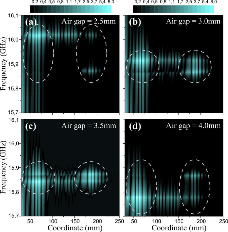
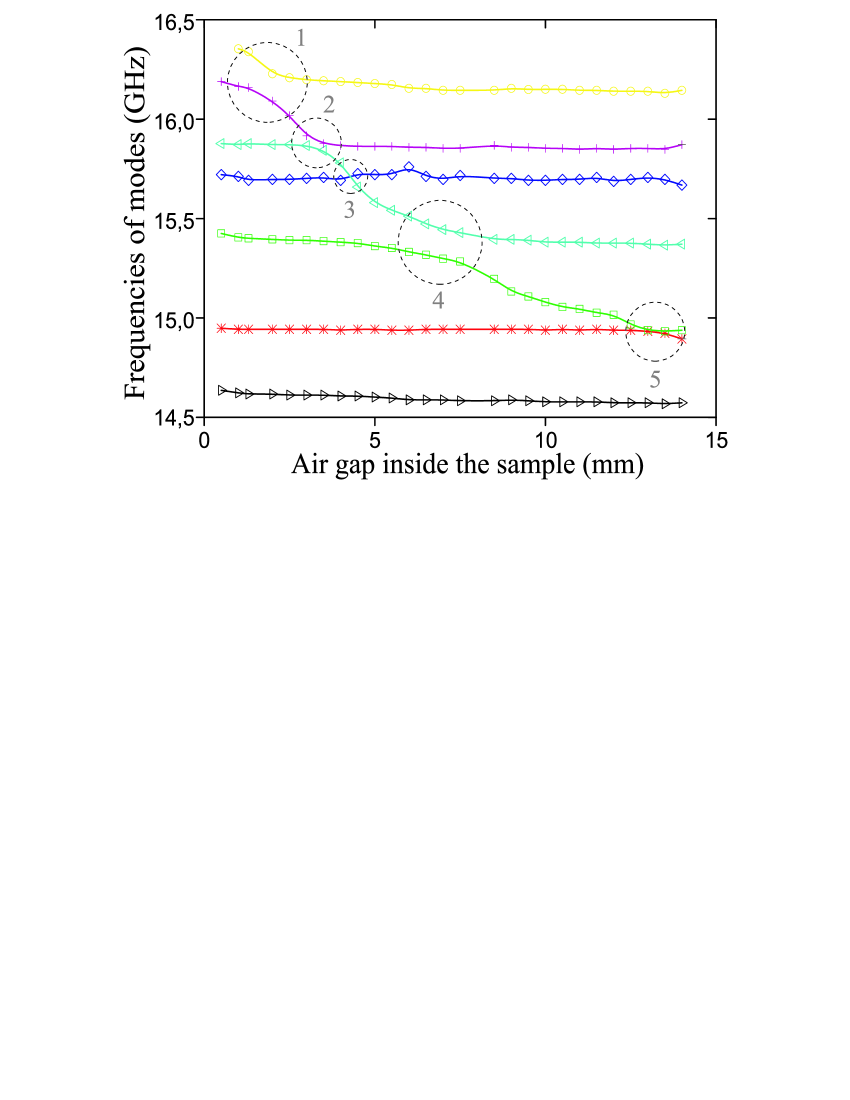
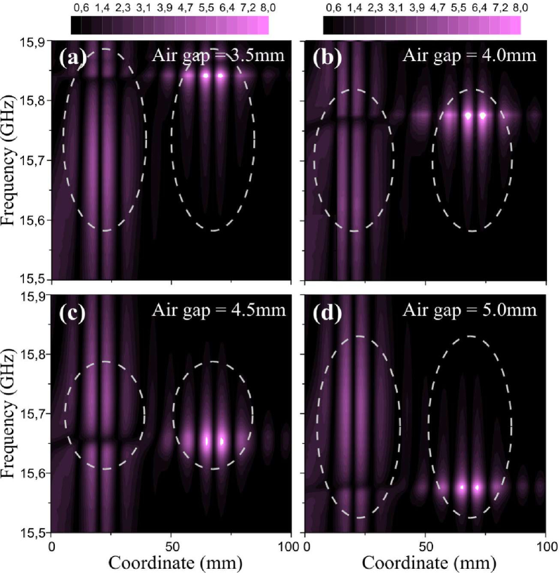
The spectral positions of the localized states as functions of the air gap introduced into the sample are plotted in Fig. 1. The frequencies of modes may cross or exhibit an anti-crossing (level repulsion). In the latter case (regions 1,2,4,5 of Fig. 1), the coupling within the sample is accompanied by an exchange of shape, as is seen in Fig. 2. When the frequencies of the modes are closest, the two localized states couple into double peaked quasi-extended modes with the same spatial intensity distribution, Fig. 2b and c. In contrast, region 3 in Fig. 1 shows a mode crossing in which the shapes are not exchanged. This is seen in Fig. 3 which shows the driven mode passing through the broad mode closest to the input. The two modes remain practically independent of each other, except for the low-intensity zone (dark horizontal line in Fig. 3) at the input mode.
Resonant wave transmission through an isolated localized state in a random sample can be described by a simple model of a wave tunneling through a resonator with semitransparent walls Azbel ; Bliokh ; Rev-Mod-Phys . Dynamics of the field in the resonator obeys the oscillator equation with an external force and damping, which accounts for the incident wave and the finite Q-factor of the resonator, respectively. Extending this model to the case of localized states which are close in frequency, we arrive at a system of coupled oscillators with the external force acting on the first of these:
| (1) |
Here is the field in the th resonator, is the dimensionless time ( is a characteristic central frequency of the problem), ( is the dimensionless eigenfrequency of th resonator, is the Q-factor describing the losses of the energy in the th resonator, is the coupling coefficient of th and th resonators due to the spatial overlap of their modes; and , ( are the amplitude and frequency of the external field exciting the first resonator. The Q-factors can be written as Yu. Bliokh :
| (2) |
where is the dissipation rate in the th resonator, are the transmission coefficient of the input and output of the system, is the wave group velocity inside the resonator cavity, and is the cavity length. The last term in Eqs. (2) accounts for the energy leakage through the outermost resonators.
To establish the correspondence between the model Eq. (1) and localized states in a random sample, we assume, following Bliokh ; Rev-Mod-Phys , that represents the peak field of the th localized state, is the amplitude of the field penetrating the adjacent cavity, and is the amplitude of the incident wave, , penetrating the first localization cavity. Since for long enough system the localization length is the only disorder-induced spatial scale in the problem, we assume
| (3) |
Here is the distance between adjacent states at coordinates and , whereas and are the distances from the edge localized states to the corresponding ends of the sample. The localization length is determined through the average value of the total transmission coefficient as [3]. The deterministic equations (1)–(3) provide an effective description of coupled modes in 1D random system.
Substituting , the set of equations (1) is reduced to an algebraic equation with
| (4) |
, and , where . The homogeneous equation determines a set of eigenmodes, with eigenfrequencies being the eigenvalues of the matrix (4).
For the sake of simplicity, we consider the case of two interacting modes, , and assume that and . Then, the complex eigenfrequencies are given by
| (5) |
This equation describes level anti-crossing and the coupling of isolated resonators to form collective eigenmodes. The minimal frequency gap is achieved at resonance, . Away from resonance, , the eigenmodes tend to the modes of isolated resonators. The shapes of the modes are exchanged when passing through the resonance, i.e., () eigenmodes correspond to the first (second) resonator at and to the second (first) resonator when . It is important to note that level repulsion of electromagnetic modes arises in a finite system in the regime of strong localization.
If the system is excited by a monochromatic wave with real frequency , as in the experiment, the complex amplitudes of the two resonators can be obtained from , which yields
| (6) | |||||
The behavior of is essentially determined by the denominator , which is at minimum at frequencies
| (7) |
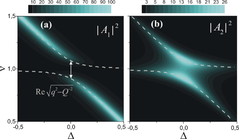
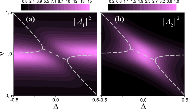
The amplitudes and frequencies characterize the resonant excitation of the system by an external source. Note that Eq. (7) coincide with Eq. (5) only in the lossless case . Otherwise, there are two different regimes of the excitation of coupled resonators, determined by the ratio between losses and coupling . If losses are small, , two branches demonstrate anti-crossing with a frequency gap , Fig. 4. If losses are greater than the coupling strength, so that , the frequencies merge in the interaction region , Fig. 5.
The amplitudes (6) for and are shown as functions of the frequency and detuning in Figs. 4 and 5, respectively. The main features observed experimentally are reproduced. Different values of correspond to different frames of Figs. 2 and 3. To facilitate comparison with the experimental results in Figs. 2 and 3, the second, output resonator is driven in Fig. 4 (, ), while the first resonator is driven in Fig. 5 (, ). It is seen in Figs. 2 and 4 that for fields in both resonators in the interaction regime (Figs. 2b and c) exhibit double-peaked spectra (level repulsion). Collective excitation of two resonators signifies the formation of quasi-extended necklace states. Remarkably, away from the resonance (Figs. 2a and d), the first resonator is effectively excited at one of the resonant frequencies, close to (Fig. 4a), while the second resonator is equally excited at both resonant frequencies (Fig. 4b). In the regime , both Figs. 3 and 5 show that the second resonator is excited with a single peak in the spectrum (Fig. 5b), while two peaks separated by a dark area driven with the frequency of the second resonator are seen in the first resonator (Fig. 5a) Note .
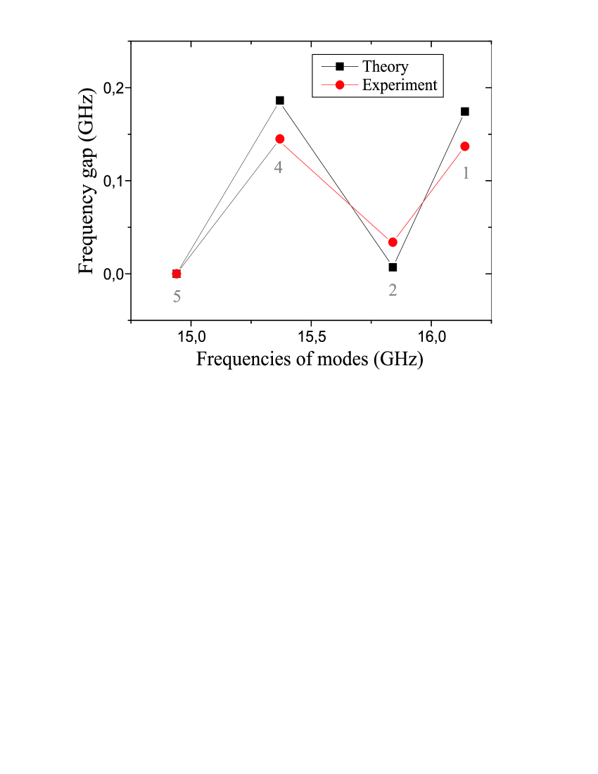
The measured and calculated values of the frequency gap between coupled modes are presented in Fig. 6. The parameters of the system are:
| (8) |
and , whereas the positions of the localized modes interacting in the regions 1–5 (Fig. 1) are equal, respectively, to
| (9) |
Substituting values (8) and (9) into Eqs. (2) and (3) yields and . We calculated the minimum frequency difference for interacting pairs 1,2,4,5 (for which Note ) as with , and compared it to measured values of the gap, Fig. 1. Good agreement between the experiment and model is seen in Fig. 6.
In conclusion, we have observed level repulsion in the localization regime and have shown that it reflects the coupling of localization centers. The occurrence of anti-crossing or crossing of quasimodes as a sample configuration changes depends upon the ratio of the coupling strength between localized states and loss. These factors determine the statistics of level spacings and widths and thus the diffusive or localized regime of wave propagation.
We thank B. Hu, J. Klosner, H. Rose, and Z. Ozimkowski for their contributions to the implementation of the waveguide assembly, and L. Pastur for illuminating discussion. This research was sponsored by the Linkage International Grant of the Australian Research Council, National Science Foundation (DMR-0538350), PSC-CUNY, the Centre National de la Recherche Scientifique (PICS and PEPS07-20), and the Groupement de Recherches IMCODE.
References
- (1) P.W. Anderson, Phys. Rev. 109, 1492 (1958).
- (2) M.Y. Azbel, Solid State Commun. 45, 527 (1983); Phys. Rev. B 28, 4106 (1983).
- (3) P. Sheng, Scattering and Localization of Classical Waves in Random Media (World Scientific, Singapore, 1990).
- (4) N.F. Mott, Phil. Mag. 22, 7 (1970).
- (5) I.M. Lifshits, and V.Y. Kirpichenkov, Zh. Eksp. Teor. Fiz. 77, 989 (1979) [Sov. Phys. JETP 50, 499 (1979)].
- (6) J.B. Pendry, J. Phys. C 20, 733 (1987); Adv. Phys. 43, 461 (1994).
- (7) J. Bertolotti et al., Phys. Rev. Lett. 94, 113903 (2005); Phys. Rev. E 74, 035602 (2006).
- (8) P. Sebbah et al., Phys. Rev. Lett. 96, 183902 (2006); J. Opt. Soc. Am. B, 24, A77 (2007).
- (9) V. Milner and A.Z. Genack, Phys. Rev. Lett. 94, 073901 (2005).
- (10) T. Guhr, A. Muller-Groeling, and H. Weidenmuller, Phys. Rep. 299, 189 (1998).
- (11) B.D. Simons and B.L. Altshuler, Phys. Rev. B 48, 5422 (1993); B.I. Shklovskii et al., ibid. 47, 11487 (1993).
- (12) L. Gor’kov,O. Dorokhov, F. Prigara, Sov. Phys. JETP 57, 838, (1983).
- (13) A.V. Malyshev, V.A. Malyshev, and J. Knoester, Phys. Rev. Lett. 98, 087401 (2007).
- (14) K.Y. Bliokh et al., J. Opt. Soc. Am. B, 21, 113 (2004); Phys. Rev. Lett. 97, 243904 (2006).
- (15) K.Y. Bliokh et al., Rev. Mod. Phys. (2008, to be published); arXiv:0708.2653.
- (16) Y.P. Bliokh, J. Felsteiner, and Y. Slutsker, Phys. Rev. Lett. 95, 165003 (2005).
- (17) It should be noted that two localized modes of Fig. 3 have significantly different Q-factors, . This diminishes the coupling between the modes since their frequencies are distant in the complex plane. Nonetheless, our simplified model with describes quantitatively all the main features of the coupling in this case.