Two-particle bound states and one-particle structure factor in a Heisenberg bilayer system

Abstract

The $S=1/2$ Heisenberg bilayer spin model at zero temperature is studied in the dimerized phase using analytic triplet-wave expansions and dimer series expansions. The occurrence of two-triplon bound states in the $S=0$ and $S=1$ channels, and antibound states in the $S=2$ channel, is predicted by the triplet-wave theory, and confirmed by series expansions. All bound states are found to vanish at or before the critical coupling separating the dimerized phase from the Néel phase. The critical behaviour of the total and single-particle static transverse structure factors is also studied by series, and found to conform with theoretical expectations. The single-particle state dominates the structure factor at all couplings.

I INTRODUCTION

Modern probes of material properties, such as the new inelastic neutron scattering facilities, are reaching such unprecedented sensitivity that they can measure the spectrum not only of a single quasiparticle excitation, but even two-particle excitations tennant2003 . These quasiparticles can collide, scatter, or form bound states just like elementary particles in free space. The spectrum of the multiparticle excitations is a crucial indicator of the underlying dynamics of the system.

One of the principal theoretical means of predicting the excitation spectrum is the method of high-order perturbation series expansions oitmaa2006 . We have previously used a ‘linked-cluster’ approach to generate series expansions for 2-particle states in 1-dimensional models trebst2000 , but for 2-dimensional models the only high-order calculations carried out so far have been those of Uhrig’s group (e.g. knetter2000 ), using the ‘continuous unitary transformation’ (CUTS) method, which is of only limited applicability. One of our aims here is to extend the linked-cluster approach to 2-dimensional models, starting with the bilayer model as a simple example.

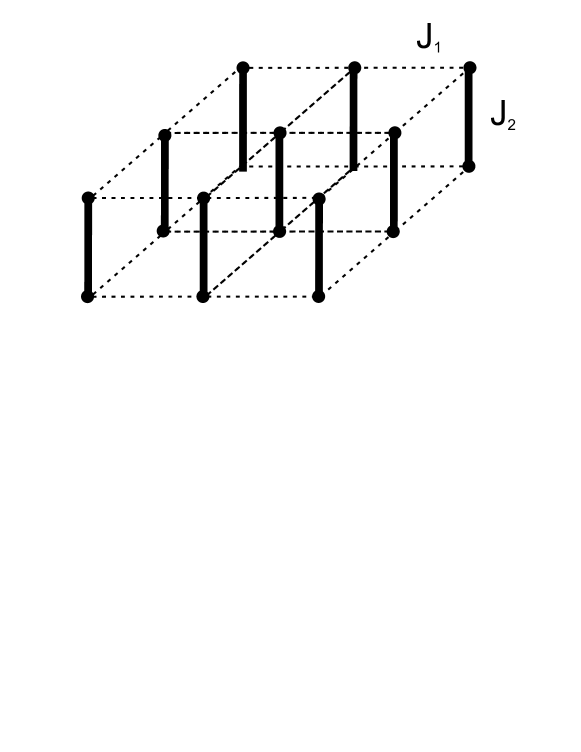
Figure 1: The bilayer Heisenberg model on a square lattice.

The $S=1/2$ bilayer Heisenberg antiferromagnet has attracted continuing interest from both experimentalists and theoreticians. Experimentally, it is of interest because many of the cuprate superconductors contain pairs of weakly coupled copper oxide layers reznik1996 ; hayden1996 ; millis1996 ; pailhes2006 . Recently, the organic material piperazinium hexachlorodicuprate has also been found to have a bilayer structure stone2006 . Theoretically, it is of particular interest because it is one of the simplest two-dimensional systems to display a dimerized, valence-bond-solid ground state, when the interplane coupling is large. There have also been discussions of the model in the presence of a magnetic field sommer2001 , or doping sandvik2002 ; pailhes2006 ; zhou2007 , or disorder sknepnek2006 .

The structure of the model is shown in Figure 1, with $S=1/2$ spins on the sites of the lattice, and Heisenberg antiferromagnetic couplings $J_{2}$ between the planes, $J_{1}$ within each plane:

$$H=J_{1}\sum_{l\ =\ 1,2}\sum_{<i,j>}{\bf S_{li}\cdot S_{lj}}+J_{2}\sum_{i}{\bf S_{1i}\cdot S_{2i}}$$ (1)

where $l=1,2$ labels the two planes of the bilayer. The physics of the system then depends on the coupling ratio $\lambda=J_{1}/J_{2}$. At $\lambda=0$, the ground state consists simply of $S=0$ dimers on each bond between the two layers, and excitations are composed of $S=1$ ‘triplon’ states on one or more bonds. At large $\lambda$, where the $J_{1}$ interaction is dominant, the ground state will be a standard Néel state, with $S=1$ ‘magnon’ excitations. At some intermediate critical value $\lambda_{c}$, a phase transition will occur between these two phases. It is believed that this transition is of second order, and is accompanied by a Bose-Einstein condensation of triplons/magnons in the ground state.

Theorists have discussed this model using series expansion methods hida1992 ; gelfand1996 ; zheng1997 , quantum Monte Carlo )QMC) simulations at small temperatures sandvik1994 ; sandvik1995 ; sandvik1996 , Schwinger-boson mean-field theory millis1993 ; miyazaki1996 , and spin-wave theory matsuda1990 ; chubukov1995 ; kotov1998 ; shevchenko1999 . The QMC analysis of Sandvik and Scalapino sandvik1996 found the transition at $\lambda_{c}=0.398(3)$, with a critical index $\nu]simeq0.7$. in agreement with the O(3) nonlinear sigma model prediction, while the exponent-biased series analysis of Zheng zheng1997 put the critical point at $\lambda_{c}=0.394(1)$. Early spin-wave estimates chubukov1995 were well away from this position, but the improved Brueckner approach of Sushkov et al. kotov1998 ; shevchenko1999 gave a remarkably accurate estimate of the critical point and critical index, and also the 1-particle dispersion in the model.

Our particular aim here is to study the two-triplon states within the dimerized regime, with particular emphasis on the occurrence of bound states, and to explore their behaviour in the vicinity of the critical point. The two-particle bound states can give important insights into the dynamical behaviour of the model. It is also possible that they may be detected experimentally at the new generation of inelastic neutron scattering facilities, or by other means.

We use two methods to investigate the two-particle states. A modified triplet-wave approach, described in Section II, gives a qualitative picture of these states, valid at small couplings $\lambda$. Series expansion calculations, sketched in Section III, are then used to obtain more accurate results, and to explore the behaviour near the critical point. Series expansions are also presented for the single-particle and total transverse structure factors. Our conclusions are summarized in Section IV.

II Modified triplet-wave theory.

Analogues of spin-wave theory in a dimerized phase have been discussed by several authors. Sachdev and Bhatt sachdev1990 used a ‘bond-operator’ representation to describe the dimers and their spin-triplet excitations, which employed both triplet and singlet operators, with a constraint between them to ensure that no two triplets can occupy the same site. The constraint is awkward to implement, and so Kotov et al. kotov1998 discarded the singlet operator, and replaced it by an infinite on-site repulsion between triplets, implemented via a self-consistent Born approximation, valid when the density of triplets is low. We have presented an alternative approach collins2006 , where the exclusion constraint is implemented automatically by means of projection operators. The absence of any constraint makes the formalism easier and more transparent to apply, but at the price of extra many-body interaction terms. This is the method used here.

The Hamiltonian for the Heisenberg bilayer systemn can be rewritten

$$H=\sum_{i}{\bf S_{1i}\cdot S_{2i}}+\lambda\sum_{1=1,2}\sum_{<i,j>}{\bf S_{\lambda i}\cdot S_{\lambda j}}$$ (2)

For $\lambda=0$, the system reduces to independent dimers as shown in Figure 1. Let us consider a single dimer with two spins ${\bf S_{1},S_{2}}$. The four states in the Hilbert space consist of a singlet and three triplet states with total spin $S=0,1$ respectively, and eigenvalues

$${\bf S_{1}\cdot S_{2}}=\left\{\begin{array}[]{cc}-3/4&(S=0)\\ +1/4&(S=1)\end{array}\right.$$ (5)

We denote the singlet ground state as $|0\rangle$, and introduce triplet creation operators that create the triplet states out of the vacuum $|0\rangle$, as follows

$$|0\rangle = \frac{1}{\sqrt{2}}[|\uparrow\downarrow\rangle-|\downarrow\uparrow\rangle]$$

$$|1,x\rangle = t^{\dagger}_{x}|0\rangle=-\frac{1}{\sqrt{2}}[|\uparrow\uparrow\rangle-|\downarrow\downarrow\rangle]$$

$$|1,y\rangle = t^{\dagger}_{y}|0\rangle=\frac{i}{\sqrt{2}}[|\uparrow\uparrow\rangle+|\downarrow\downarrow\rangle]$$

$$|1,z\rangle = t^{\dagger}_{z}|0\rangle=\frac{1}{\sqrt{2}}[|\uparrow\downarrow\rangle+|\downarrow\uparrow\rangle]$$ (6)

Then the spin operators ${\bf S_{1}}$ and ${\bf S_{2}}$ can be represented in terms of triplet operators by

$$S_{1\alpha} = \frac{1}{2}[t^{\dagger}_{\alpha}(1-t^{\dagger}_{\gamma}t_{\gamma})+(1-t^{\dagger}_{\gamma}t_{\gamma})t_{\alpha}-i\epsilon_{\alpha\beta\gamma}t^{\dagger}_{\beta}t_{\gamma}]$$

$$S_{2\alpha} = \frac{1}{2}[-t^{\dagger}_{\alpha}(1-t^{\dagger}_{\gamma}t_{\gamma})-(1-t^{\dagger}_{\gamma}t_{\gamma})t_{\alpha}$$ (7)

$$-i\epsilon_{\alpha\beta\gamma}t^{\dagger}_{\beta}t_{\gamma}]$$

where $\alpha,\beta,\gamma$ take the values $x,y,z$ and repeated indices are summed over. This is similar to the representation of Sachdev and Bhatt sachdev1990 , except that we have omitted singlet operators $s^{\dagger},s$, but used projection operators $(1-t^{\dagger}_{\gamma}t_{\gamma})$ instead. Assume the triplet operators obey bosonic commutation relations

$$[t_{\alpha},t^{\dagger}_{\beta}]=\delta_{\alpha\beta},$$ (8)

then one can show that within the physical subspace (i.e. total number of triplet states is 0 or 1), the representation (7) obeys the correct spin operator algebra

$$[S_{1\alpha},S_{1\beta}]=i\epsilon_{\alpha\beta\gamma}S_{1\gamma},\hskip 14.22636pt[S_{2\alpha},S_{2\beta}]=i\epsilon_{\alpha\beta\gamma}S_{2\gamma},$$

$$[S_{1\alpha},S_{2\beta}]=0$$ (9)

$${\bf S}_{1}^{2}={\bf S}_{2}^{2}=3/4,\hskip 14.22636pt{\bf S_{1}\cdot S_{2}}=t^{\dagger}_{\alpha}t_{\alpha}-3/4$$ (10)

The projection operators ensure that we remain within the subspace.

Returning to the bilayer system, we can now define triplet operators $t^{\dagger}_{n\alpha},t_{n\alpha}$ for each dimer $n$ in the system. For a system of $N$ dimers, the Hamiltonian now can be expressed in terms of triplet operators as

$$H = -\frac{3N}{4}+\sum_{n}t^{\dagger}_{n\alpha}t_{n\alpha}+\frac{\lambda}{2}\sum_{<ij>}\{t^{\dagger}_{i\alpha}t^{\dagger}_{j\alpha}+t_{i\alpha}t_{j\alpha}+t_{i\alpha}t^{\dagger}_{j\alpha}+t^{\dagger}_{i\alpha}t_{j\alpha}\}-\frac{\lambda}{2}\sum_{<ij>}\{(t^{\dagger}_{i\alpha}t^{\dagger}_{i\beta}t_{i\beta}+t^{\dagger}_{i\beta}t_{i\beta}t_{i\alpha})(t^{\dagger}_{j\alpha}+t_{j\alpha})$$ (11)

$$+(t^{\dagger}_{i\alpha}+t_{i\alpha})(t^{\dagger}_{j\alpha}t^{\dagger}_{j\beta}t_{j\beta}+t^{\dagger}_{j\beta}t_{j\beta}t_{j\alpha})+t^{\dagger}_{i\alpha}t_{i\beta}t^{\dagger}_{j\alpha}t_{j\beta}-t^{\dagger}_{i\alpha}t_{i\beta}t^{\dagger}_{j\beta}t_{j\alpha}\}$$

$$+\frac{\lambda}{2}\sum_{<ij>}\{(t^{\dagger}_{i\alpha}t^{\dagger}_{i\beta}t_{i\beta}+t^{\dagger}_{i\beta}t_{i\beta}t_{i\alpha})(t^{\dagger}_{j\alpha}t^{\dagger}_{j\gamma}t_{j\gamma}+t^{\dagger}_{j\gamma}t_{j\gamma}t_{j\alpha})\}$$

This expression includes terms containing up to 6 triplet operators.

Next, perform a Fourier transform

$$t_{{\bf k}\alpha} = (\frac{1}{N})^{1/2}\sum_{\bf n}e^{i{\bf k.n}}t_{{\bf n}\alpha}$$

$$t^{\dagger}_{{\bf k}\alpha} = (\frac{1}{N})^{1/2}\sum_{\bf n}e^{-i{\bf k.n}}t^{\dagger}_{{\bf n}\alpha}$$ (12)

(we set the spacing between dimers $d=1$), then the Hamiltonian becomes

$$H = -\frac{3N}{4}+\sum_{{\bf k}}t^{\dagger}_{{{\bf k}}\alpha}t_{{\bf k}\alpha}+\lambda\sum_{{\bf k}}\gamma_{{\bf k}}[t^{\dagger}_{{\bf k}\alpha}t^{\dagger}_{-{\bf k}\alpha}+t_{{\bf k}\alpha}t_{-{\bf k}\alpha}+2t^{\dagger}_{{\bf k}\alpha}t_{{\bf k}\alpha}]$$ (13)

$$-\frac{\lambda}{N}\sum_{1234}\{\delta_{1+2+3-4}[(t^{\dagger}_{1\alpha}t^{\dagger}_{2\alpha}t^{\dagger}_{3\gamma}t_{4\gamma}+t^{\dagger}_{4\gamma}t_{3\gamma}t_{2\alpha}t_{1\alpha})(\gamma_{1}+\gamma_{2})]+\delta_{1+2-3-4}[t^{\dagger}_{1\alpha}t^{\dagger}_{2\gamma}t_{3\alpha}t_{4\gamma}(\gamma_{1}+\gamma_{2}+\gamma_{3}+\gamma_{4})$$

$$+\gamma_{{\bf 1-3}}t^{\dagger}_{1\beta}t^{\dagger}_{2\beta}t_{3\gamma}t_{4\gamma}-\gamma_{{\bf 1-4}}t^{\dagger}_{1\beta}t^{\dagger}_{2\gamma}t_{3\beta}t_{4\gamma})]\}$$

$$+\frac{\lambda}{N^{2}}\sum_{1-6}\{\delta_{1+2+3+4-5-6}[\gamma_{{\bf 3+4-6}}(t^{\dagger}_{1\alpha}t^{\dagger}_{2\gamma}t^{\dagger}_{3\alpha}t^{\dagger}_{4\beta}t_{5\gamma}t_{6\beta}+t^{\dagger}_{6\beta}t^{\dagger}_{5\gamma}t_{4\beta}t_{3\alpha}t_{2\gamma}t_{1\alpha})]$$

$$+\delta_{1+2+3-4-5-6}t^{\dagger}_{1\alpha}t^{\dagger}_{2\beta}t^{\dagger}_{3\gamma}t_{4\gamma}t_{5\beta}t_{6\alpha}(\gamma_{{\bf 3-4-6}}+\gamma_{{\bf 2+3-4}})\}$$

where the indices $1-6$ are shorthand for momenta ${\bf k_{1}}-{\bf k_{6}}$, and

$$\gamma_{\bf k}=\frac{1}{2}(\cos k_{x}+\cos k_{y})$$ (14)

for the square lattice. Henceforward, we drop the 6-particle terms.

Finally, as in a standard spin-wave analysis, we perform a Bogoliubov transform

$$t_{{\bf k}\alpha}=c_{{\bf k}}\tau_{{\bf k}\alpha}+s_{\bf k}\tau^{\dagger}_{-{\bf k}\alpha}$$ (15)

where $c_{\bf k}=\cosh\theta_{\bf k}$, $s_{\bf k}=\sinh\theta_{\bf k}$, $\theta_{-{\bf k}}=\theta_{\bf k}$, which preserves the boson commutation relations

$$[\tau_{{\bf k}\alpha},\tau^{\dagger}_{{\bf k}^{\prime}\beta}]=\delta_{{\bf k}{\bf k}^{\prime}}\delta_{\alpha\beta}$$ (16)

and is intended to diagonalize the Hamiltonian up to quadratic terms. After normal ordering, the transformed Hamiltonian up to fourth order terms reads

$$H=W_{0}+H_{2}+H_{3}+H_{4},$$ (17)

where the constant term is

$$W_{0} = 3N\left\{-\frac{1}{4}+R_{2}+2\lambda(R_{3}+R_{4})-2\lambda[2(R_{3}+R_{4})(R_{1}+4R_{2})+\frac{1}{N^{2}}\sum_{12}\gamma_{{\bf 1-2}}(c_{1}s_{1}c_{2}s_{2}-s_{1}^{2}s_{2}^{2})]\right.$$ (18)

$$\left.+2\lambda[(R_{3}+R_{4})(R_{1}+4R_{2})^{2}+\frac{1}{N^{3}}\sum_{123}\gamma_{{\bf 1+2-3}}(c_{1}s_{1}(4c_{2}s_{2}c_{3}s_{3}+6c_{2}s_{2}s_{3}^{2}+6s_{2}^{2}s_{3}^{2})+4s_{1}^{2}s_{2}^{2}s_{3}^{2})]\right\}$$

expressed in terms of the momentum sums

$$R_{1} = \frac{1}{N}\sum_{{\bf k}}c_{{\bf k}}s_{{\bf k}}$$

$$R_{2} = \frac{1}{N}\sum_{{\bf k}}s_{{\bf k}}^{2}$$

$$R_{3} = \frac{1}{N}\sum_{{\bf k}}c_{{\bf k}}s_{{\bf k}}\gamma_{{\bf k}}$$

$$R_{4} = \frac{1}{N}\sum_{{\bf k}}s_{{\bf k}}^{2}\gamma_{{\bf k}}.$$ (19)

The quadratic terms are

$$H_{2}=\sum_{{\bf k},\alpha}[E_{{\bf k}}\tau^{\dagger}_{{\bf k}\alpha}\tau_{{\bf k}\alpha}+Q_{\bf k}(\tau_{{\bf k}\alpha}\tau_{-{\bf k}\alpha}+\tau^{\dagger}_{{\bf k}\alpha}\tau^{\dagger}_{-{\bf k}\alpha})]$$ (20)

where

$$E_{{\bf k}} = (c_{{\bf k}}^{2}+s_{{\bf k}}^{2})(1+2\lambda\gamma_{{\bf k}})+4\lambda\gamma_{{\bf k}}c_{{\bf k}}s_{{\bf k}}$$ (21)

$$-\lambda[4(c_{{\bf k}}^{2}+s_{{\bf k}}^{2})(\gamma_{{\bf k}}(R_{1}+4R_{2})+4(R_{3}+R_{4})-\frac{1}{N}\sum_{1}s_{1}^{2}\gamma_{{\bf k-1}})$$

$$+8c_{{\bf k}}s_{{\bf k}}(\gamma_{{\bf k}}(R_{1}+4R_{2})+(R_{3}+R_{4})+\frac{1}{N}\sum_{1}c_{1}s_{1}\gamma_{{\bf k-1}})]$$

$$Q_{{\bf k}} = c_{{\bf k}}s_{{\bf k}}(1+2\lambda\gamma_{{\bf k}})+\lambda\gamma_{{\bf k}}(c_{{\bf k}}^{2}+s_{{\bf k}}^{2})$$ (22)

$$-\lambda[2(c_{{\bf k}}^{2}+s_{{\bf k}}^{2})(\gamma_{{\bf k}}(R_{1}+4R_{2})+(R_{3}+R_{4})+\frac{1}{N}\sum_{1}c_{1}s_{1}\gamma_{{\bf k}-{\bf 1}})$$

$$+4c_{{\bf k}}s_{{\bf k}}(\gamma_{{\bf k}}(R_{1}+4R_{2})+4(R_{3}+R_{4})-\frac{1}{N}\sum_{1}s_{1}^{2}\gamma_{\bf k-1})]$$

The fourth-order terms are

$$H_{4} = -\frac{\lambda}{N}\sum_{1234}[\delta_{1+2+3+4}\Phi^{(1)}_{4}(\tau^{\dagger}_{1\alpha}\tau^{\dagger}_{2\alpha}\tau^{\dagger}_{3\gamma}\tau^{\dagger}_{4\gamma}+\tau_{1\alpha}\tau_{2\alpha}\tau_{3\gamma}\tau_{4\gamma})+\delta_{1+2-3-4}(\Phi^{(2)}_{4}\tau^{\dagger}_{1\alpha}\tau^{\dagger}_{2\alpha}\tau_{3\gamma}\tau_{4\gamma}+\Phi_{4}^{(3)}\tau^{\dagger}_{1\alpha}\tau^{\dagger}_{2\gamma}\tau_{3\alpha}\tau_{4\gamma})$$ (23)

$$+\delta_{1+2+3-4}\Phi^{(4)}_{4}(\tau^{\dagger}_{1\alpha}\tau^{\dagger}_{2\alpha}\tau^{\dagger}_{3\gamma}\tau_{4\gamma}+\tau^{\dagger}_{4\gamma}\tau_{3\gamma}\tau_{2\alpha}\tau_{1\alpha})]$$

where we have used the shorthand notation $1\cdots 4$ for momenta $k_{1}\cdots k_{4}$, and the vertex functions $\Phi^{(i)}_{4}$ are listed in Appendix A. These results were obtained or confirmed using a symbolic manipulation program written in PERL.

The condition that the off-diagonal quadratic terms vanish is

$$Q_{{\bf k}}=0.$$ (24)

In a conventional spin-wave approach, this would be implemented in leading order only, giving the condition

$$\tanh 2\theta_{{\bf k}}=\frac{2s_{{\bf k}}c_{{\bf k}}}{c_{{\bf k}}^{2}+s_{{\bf k}}^{2}}=-\frac{2\lambda\gamma_{{\bf k}}}{[1+2\lambda\gamma_{{\bf k}})}$$ (25)

This would leave some residual off-diagonal quadratic terms, arising from the normal-ordering of quartic operators. In a ‘modified’ approach gochev1994 , we demand that these terms vanish entirely up to the order calculated, giving the modified condition

$$\tanh 2\theta_{{\bf k}}=-\frac{2\lambda[\gamma_{{\bf k}}-2(\gamma_{{\bf k}}(R_{1}+4R_{2})+(R_{3}+R_{4})+\frac{1}{N}\sum_{1}c_{1}s_{1}\gamma_{{\bf k-1}})]}{[1+2\lambda(\gamma_{{\bf k}}-2(\gamma_{{\bf k}}(R_{1}+4R_{2})+4(R_{3}+R_{4})-\frac{1}{N}\sum_{1}s_{1}^{2}\gamma_{{\bf k-1}}))]}$$ (26)

Self-consistent solutions for the N equations (26), with the four parameters $R_{1}\cdots R_{4}$ given by equation (19), can easily be found by numerical means, starting from the conventional result (25).

II.1 Expansion in powers of $\lambda$

As a first check on the formalism, one may calculate the leading terms in an expansion of the energy eigenvalues in powers of $\lambda$. Solving the modified equation (26) self-consistently to order $\lambda^{2}$, we find

$$s_{{\bf k}} = -\lambda\gamma_{{\bf k}}+\frac{\lambda^{2}}{2}(4\gamma_{{\bf k}}^{2}-\gamma_{{\bf k}}-1)$$

$$c_{{\bf k}} = 1+\frac{1}{2}\lambda^{2}\gamma_{{\bf k}}^{2}$$ (27)

with the lattice sums (19)

$$R_{1} = O(\lambda^{4}),\hskip 14.22636ptR_{2}=\frac{\lambda^{2}}{4}+\frac{\lambda^{3}}{4}+O(\lambda^{4}),$$

$$R_{3} = -\frac{\lambda}{4}-\frac{\lambda^{2}}{8}+O(\lambda^{3}),\hskip 14.22636ptR_{4}=O(\lambda^{3})$$ (28)

The leading-order behaviour of the vertex functions may easily be deduced from Appendix A.

Substituting in equation (18), the ground state energy per dimer is

$$\epsilon_{0} = \frac{W_{0}}{N}\sim-3[\frac{1}{4}+\frac{\lambda^{2}}{4}+\frac{\lambda^{3}}{8}]\hskip 14.22636pt\lambda\rightarrow 0$$ (29)

in agreement with dimer series expansion results previously obtained for this model zheng1997 . One can easily show that perturbation diagrams such as those in Figure 2 do not contribute until $O(\lambda^{4})$ or higher.

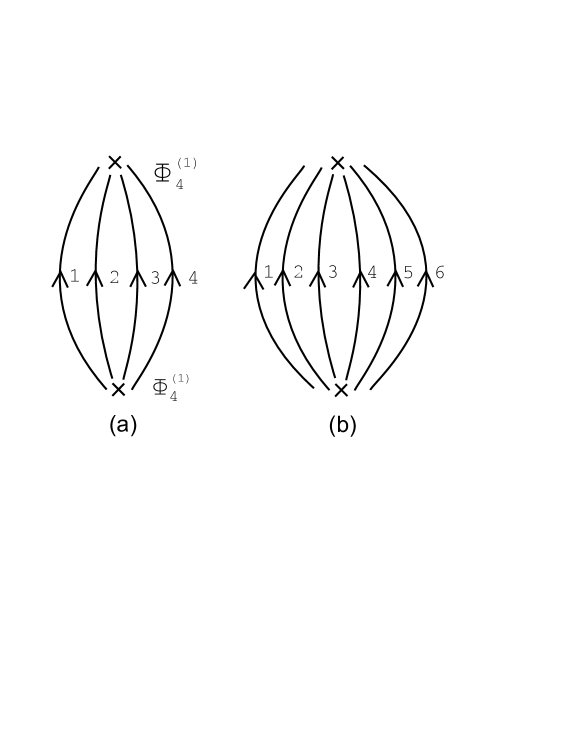
Figure 2: Perturbation diagrams contributing to the ground-state energy.

The energy gap at leading order can be found from equation (21):

$$E_{k}\sim 1+2\lambda\gamma_{{\bf k}}+4\lambda^{2}-2\lambda^{2}\gamma_{{\bf k}}^{2}\hskip 14.22636pt\lambda\rightarrow 0$$ (30)

Note that in linear spin-wave theory, when $\tanh 2\theta_{{\bf k}}$ is given by (25) and the energy gap is given by the first line of equation (21), the energy gap is

$$E_{k}=\sqrt{1+4\lambda\gamma_{{\bf k}}}$$ (31)

which vanishes at $\lambda=1/4,\gamma_{{\bf k}}=-1$, i.e. ${\bf k}=(\pi,\pi)$. This marks a phase transition with critical index $\nu=1/2$, and the end of the dimerized phase, in this approximation.

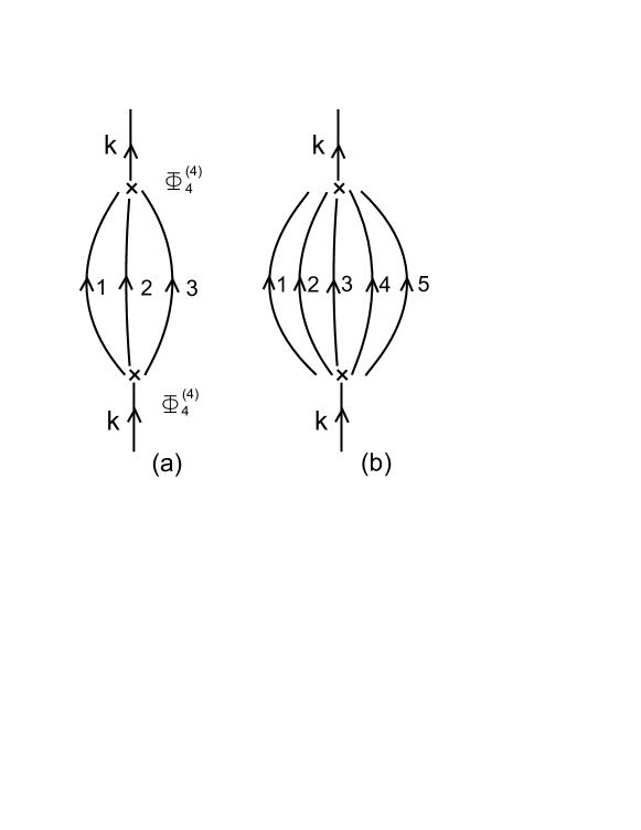
Figure 3: Perturbation diagrams contributing to the one-particle energy.

The perturbation diagram Figure 3a) also contributes to the energy gap at order $\lambda^{2}$. Note that diagram 3a) does not appear in the formalism of Shevchenko et al. shevchenko1999 ; kotov1998 ; the extra terms in our formalism are needed to implement the hardcore constraint that two triplons cannot occupy the same site. At leading order, the contribution of this diagram is

$$\Delta E_{k}^{3a)}\sim-2\lambda^{2}\hskip 14.22636pt\lambda\rightarrow 0$$ (32)

(see the next section for further details). This gives a total single-particle energy

$$\epsilon_{k}\sim 1+2\lambda\gamma_{{\bf k}}+2\lambda^{2}(1-\gamma_{{\bf k}}^{2}),\hskip 14.22636pt\lambda\rightarrow 0$$ (33)

which again agrees with series expansion results zheng1997 .

The minimum energy gap lies at ${\bf k}=(\pi,\pi)$. If we compare equation (33) at small momentum ${\bf p}=(\pi,\pi)-{\bf k}$ with the continuum dispersion relation for a free boson,

$$\epsilon_{k}\sim\sqrt{m^{2}c^{4}+p^{2}c^{2}}$$ (34)

we readily discover the leading behaviour of the effective triplon parameters, i.e. the triplon mass

$$m\sim\frac{1}{\lambda}[1-2\lambda+O(\lambda^{2})]$$ (35)

and the ‘speed of light’ or triplon velocity

$$c^{2}\sim\lambda+O(\lambda^{3})$$ (36)

in lattice units. Note that the mass diverges and the speed of light vanishes as $\lambda\rightarrow 0$.

II.2 Numerical Results

Writing the Hamiltonian as

$$H=H_{0}+V$$ (37)

where

$$H_{0}=W_{0}+H_{2}$$ (38)

and

$$V=H_{4}$$ (39)

(6-particle terms being neglected) we can treat $H_{0}$ as the unperturbed Hamiltonian and $V$ as a perturbation to obtain the leading-order corrections to the predictions for physical quantities outlined in the previous section. Numerical results for the model have been obtained using the finite-lattice method. The momentum sums are carried out for a fixed lattice size $L\times L=N$, using corresponding discrete values for the momentum ${\bf k}$, e.g.

$$k_{x} = \frac{2\pi n}{L},\hskip 14.22636ptn=1,\cdots L$$

$$k_{y} = \frac{2\pi m}{L},\hskip 14.22636ptm=1,\cdots L$$ (40)

Results were obtained for $L$ up to 100.

II.2.1 Ground-state energy

Figure 4: Ground-state energy per dimer as a function of $\lambda$. The solid line is the estimate from series expansions, and the dashed line is the triplet-wave estimate.

The leading correction to the ground-state energy corresponds to the diagram in Figure 2a). Its contribution is

$$\Delta\epsilon_{0}^{2a)} = \frac{-3\lambda^{2}}{N^{3}}\sum_{1234}\delta_{1+2+3+4}\frac{\Phi_{4}^{(1)}(1234)}{(E_{1}+E_{2}+E_{3}+E_{4})}\left[3\Phi_{4}^{(1)}(1234)+\Phi_{4}^{(1)}(1324)+\Phi_{4}^{(1)}(1423)\right]$$ (41)

In leading order one can show that this term is $O(\lambda^{4})$, whereas diagrams such as Figure 2b) are $O(\lambda^{6})$ or higher. Figure 4 shows the behaviour of the ground-state energy as a function of $\lambda$ resulting from this modified triplon theory, as compared with the high-order dimer series calculations of Zheng zheng1997 . It can be seen that out to $\lambda\simeq 0.1$ there is quantitative agreement between our calculation and the series estimates, but some discrepancy emerges at larger $\lambda$.

II.2.2 One-particle spectrum

The leading correction to the one-particle spectrum corresponds to the diagram in Figure 3a). Its contribution is

$$\Delta E_{k}^{3a)} = \frac{2\lambda^{2}}{N^{2}}\sum_{123}\delta_{{\bf 1+2+3-k}}\frac{\Phi_{4}^{(4)}(123k)}{(E_{k}-E_{1}-E_{2}-E_{3})}\left[3\Phi_{4}^{(4)}(123k)+\Phi_{4}^{(4)}(321k)+\Phi_{4}^{(4)}(312k)\right]$$ (42)

In leading order, this term is $O(\lambda^{2})$, as stated in the previous section, while diagrams like 3b) are $O(\lambda^{4})$ or higher.

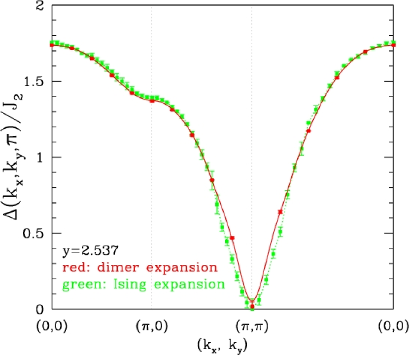
Figure 5: [Colour online] One-particle dispersion relation at the critical point ($y=1/\lambda$), as estimated from both dimer (solid line) and Ising (dashed line) expansions zheng1997 .

The dispersion of the one-particle energy as a function of momentum ${\bf k}$ at the critical point is illustrated in Figure 5, as estimated from two different series expansions by Zheng zheng1997 . It can be seen that the two expansions agree well at the critical point, and that the energy gap vanishes there at the Néel point ${\bf k}=(\pi,\pi)$.

Figure 6: Energy gap at ${\bf k}=(\pi,\pi)$ as a function of $\lambda$. The solid squares show the series estimates zheng1997 , and the open squares are results from Shevchenko et al. shevchenko1999 , while the stars show the improved triplet-wave results. The contributions from 2-triplon and 4-triplon terms are shown separately.

The triplet-wave and series estimates of the energy gap at ${\bf k}=(\pi,\pi)$ are compared in Figure 6. It can be seen that the inclusion of the corrections from diagram 3a) improves the agreement with series substantially, bringing quantitative agreement out to $\lambda\simeq 0.15$. Beyond that, the triplet-wave estimates begin to diverge, as higher-order contributions become more important. The self-consistent Born approach of Kotov et al. kotov1998 ; shevchenko1999 is more accurate than our approach at large $\lambda$; but neither approach can compete with series methods for accuracy. Our object here mainly is to understand the qualitative behaviour of the model.

II.2.3 Two-triplon bound states

It has been found in previous studies of dimerized antiferromagnetic systems in one dimension uhrig1996 ; shevchenko1999 that the quartic terms in the Hamiltonian lead to attraction between two elementary triplons, giving rise to $S=0$ and $S=1$ bound states. We look for solutions of the two-body Schrödinger equation

$$H|\psi\rangle=E|\psi\rangle.$$ (43)

The two-body wave functions $|\psi({\bf K})\rangle$ can be written as follows:

Singlet sector ($S=0$):

$$|\psi^{S}({\bf K})\rangle=\frac{1}{\sqrt{6}}\sum_{{\bf q},\alpha}\psi^{S}({\bf K},{\bf q})\tau^{\dagger}_{{\bf K}/2+{\bf q},\alpha}\tau^{\dagger}_{{\bf K}/2-{\bf q},\alpha}|0\rangle$$ (44)

where ${\bf K}$ is the centre-of-mass momentum and ${\bf q}$ the relative momentum of the two particles, and the scalar wave function is symmetric,

$$\psi^{S}({\bf K},-{\bf q})=\psi^{S}({\bf K},{\bf q})$$ (45)

Triplet sector ($S=1$):

$$|\psi^{T}_{\alpha}({\bf K})\rangle=\frac{1}{2}\sum_{{\bf q},\beta,\gamma}\epsilon_{\alpha\beta\gamma}\psi^{T}({\bf K},{\bf q})\tau^{\dagger}_{{\bf K}/2+{\bf q},\beta}\tau^{\dagger}_{{\bf K}/2-{\bf q},\gamma}|0\rangle$$ (46)

with the wave function antisymmetric

$$\psi^{T}({\bf K},-{\bf q})=-\psi^{T}({\bf K},{\bf q}).$$ (47)

We will not write out the quintuplet states explicitly.

From equation (43) one can readily derive the integral Bethe-Salpeter equation satisfied by the bound-state wave functions:

$$[E^{S,T,Q}({\bf K})-E_{{\bf K}/2+{\bf q}}-E_{{\bf K}/2-{\bf q}}]\psi^{S,T,Q}({\bf K},{\bf q})=$$

$$\frac{1}{N}\sum_{{\bf p}}M^{S,T,Q}({\bf K},{\bf q},{\bf p})\psi^{S,T,Q}({\bf K},{\bf p})$$ (48)

in each sector S,T or Q.

In leading order, the scattering amplitudes $M^{S,T,Q}({\bf K},{\bf q},{\bf p})$ are simply given by the 4-particle vertex from the perturbation operator $V$, Figure 7a). Hence we find for the different sectors:

$$M^{S}({\bf K},{\bf q},{\bf p})=-2\lambda[3\Phi^{(2)}_{4}({\bf K}/2+{\bf q},{\bf K}/2-{\bf q},{\bf K}/2+{\bf p},{\bf K}/2-{\bf p})+\Phi^{(3)+}_{4}({\bf{\bf K}}/2+{\bf q},{\bf{\bf K}}/2-{\bf q},{\bf K}/2+{\bf p},{\bf K}/2-{\bf p})]$$ (49)

$$M^{T}({\bf K},{\bf q},{\bf p})=-2\lambda\Phi^{(3)-}_{4}({\bf K}/2+{\bf q},{\bf K}/2-{\bf q},{\bf K}/2+{\bf p},{\bf K}/2-{\bf p})$$ (50)

$$M^{Q}({\bf K},{\bf q},{\bf p})=-2\lambda\Phi^{(3)+}_{4}({\bf K}/2+{\bf q},{\bf K}/2-{\bf q},{\bf K}/2+{\bf p},{\bf K}/2-{\bf p})$$ (51)

where the wave function is once again symmetric in the quintuplet sector

$$\psi^{Q}({\bf K},-{\bf q})=\psi^{Q}({\bf K},{\bf q}).$$ (52)

and the symmetric and antisymmetric pieces of the vertex function $\Phi_{4}^{(3)}$ are defined:

$$\Phi^{(3)\pm}_{4}\equiv\frac{1}{2}[\Phi^{(3)}_{4}(1234)\pm\Phi^{(3)}_{4}(1243)].$$ (53)

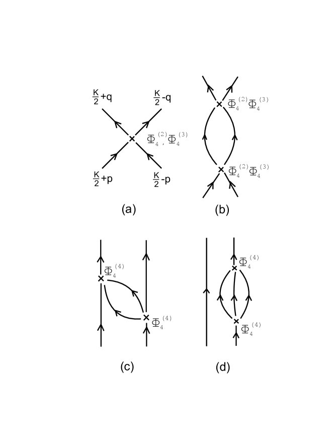
Figure 7: Perturbation diagrams contributing to the 2-particle scattering amplitude.

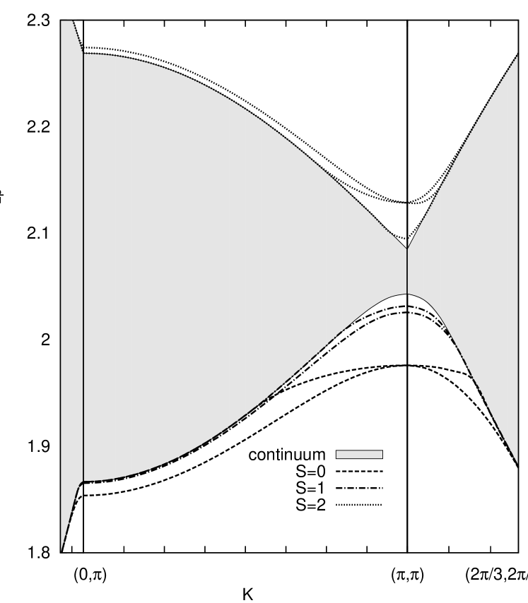
Figure 8: [Color online] Dispersion relations for the two-particle bound/antibound states at $\lambda=0.1$, along symmetry lines in the Brillouin zone, as calculated from the triplet-wave expansion. The 2-particle continuum region is shaded.

At leading order in $\lambda$, we find

$$M^{S}({\bf K},{\bf q},{\bf p}) \sim -2\lambda[\gamma_{{\bf p+q}}+\gamma_{{\bf p-q}}+\gamma_{{\bf K}/2+{\bf p}}$$ (54)

$$+\gamma_{{\bf K}/2+{\bf q}}+\gamma_{{\bf K}/2-{\bf p}}+\gamma_{{\bf K}/2-{\bf q}}]$$

$$M^{T}({\bf K,q,p})\sim\lambda[\gamma_{{\bf q+p}}-\gamma_{{\bf q-p}}]$$ (55)

and

$$M^{Q}({\bf K,q,p}) \sim \lambda[\gamma_{{\bf q+p}}+\gamma_{{\bf q-p}}-2(\gamma_{{\bf K}/2+{\bf p}}$$ (56)

$$+\gamma_{{\bf K}/2+{\bf q}}+\gamma_{{\bf K}/2-{\bf p}}+\gamma_{{\bf K}/2-{\bf q}})]$$

Then restricting ourselves to the particular momentum ${\bf K}=(\pi,\pi)$, simple solutions to the Bethe-Salpeter equation (48) can be found:

$$\Psi^{S,Q}({\bf K,q}) \sim (\cos q_{x}\pm\cos q_{y})$$

$$\Psi^{T}({\bf K,q}) \sim (\sin q_{x}\pm\sin q_{y})$$ (57)

corresponding to nearest-neighbour pairs of triplon excitations, with energies:

$$E^{S}({\bf K}) \sim 2-\lambda$$

$$E^{T}({\bf K}) \sim 2-\lambda/2$$

$$E^{Q}({\bf K}) \sim 2+\lambda/2$$ (58)

Since the 2-particle continuum is confined strictly to $E_{cont}=2$ at this order and this momentum, we see that the singlet and triplet states are bound states lying below the continuum, while the quintuplet states are antibound states lying above the continuum. There are two degenerate states in each case, corresponding to the $\pm$ signs in equation (57), or to the two possible axes $x$ and $y$ of the nearest-neighbour pairs. At higher orders these states may mix and separate.

These results are easily understood in a qualitative fashion. For an $S^{z}=2$ excitation, for example, the spins on the nearest-neighbour sites are necessarily aligned parallel, giving rise to a repulsive interaction; whereas for $S=0$ or 1 the neighbouring spins can be aligned either parallel or antiparallel, allowing the possibility of an attractive interaction.

Solving the wave equation (48) with vertex functions given by the leading order approximations (49) - (51), we obtain numerical solutions for the 2-particle spectrum, as illustrated in Figure 8, at a coupling $\lambda=0.1$, near momentum ${\bf k}=(\pi,\pi)$. It can be seen that the pairs of degenerate $S=0$ and $S=2$ bound/antibound states split as one moves away from $(\pi,\pi)$, and all states eventually merge into the continuum.

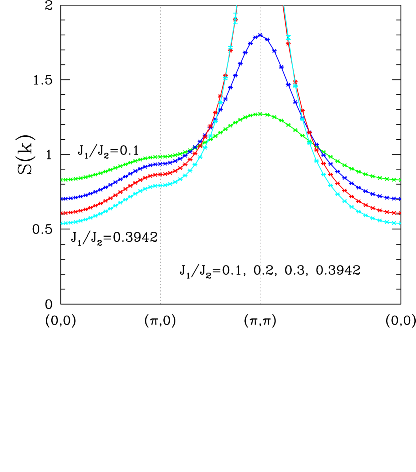
Figure 9: [Color online] The total static structure factor $S({\bf k})$ as a function of ${\bf k}$, for various couplings $\lambda=J_{1}/J_{2}$.

III Series Expansions

We have performed a standard dimer series expansion singh1988 ; oitmaa2006 for this model, where the Hamiltonian is written as

$$H = H_{0}+\lambda V$$ (59)

$$H_{0} = \sum_{i}{\bf S_{1i}\cdot S_{2i}}$$ (60)

$$V = \sum_{l=1,2}\sum_{<ij>}{\bf S_{li}\cdot S_{lj}}$$ (61)

and perturbation series are generated for the quantities of interest in powers of $\lambda$, using linked cluster methods. Details of the linked cluster approach are reviewed in oitmaa2006 . In very brief summary, the ground-state energy per dimer can be written as a sum of the irreducible contributions (cumulants) coming from every connected cluster of dimers which can be embedded on the lattice, the order of the contributions rising with the size of the cluster. The 1-particle energies can be written in terms of irreducible transition amplitudes $\Delta_{1}(i,j)$ of the effective Hamiltonian gelfand1996 , which consist of a sum over all linked clusters connected to $i$ and $j$, the initial and final positions of the 1-particle excitations. And finally, the 2-particle energies can be written in terms of irreducible transition amplitudes $\Delta_{2}(i,j;k,l)$ of the 2-particle effective Hamiltonian trebst2000 , consisting of a sum over all linked clusters connected to $(i,j)$ and $(k,l)$, the initial and final positions of the 2-particle excitations. The amplitudes $\Delta_{2}$ are then employed in the 2-particle Schrödinger or Bethe-Salpeter equation to calculate the energy for as a function of momentum. We use a finite-lattice approach oitmaa2006 for this purpose, where the Schrödinger equation is solved on a finite lattice in position space, of sufficient size to ensure convergence of the results.

Once a perturbation series in $\lambda$ has been calculated for a given quantity, it can be extrapolated to finite $\lambda$ using Padé approximants or integrated differential approximants.

Zheng zheng1997 has previously calculated series for the ground-state energy and 1-particle excitations. These results have already been compared with the triplet-wave predictions in Figures 4, 5 and 6.

III.1 Structure Factors

Figures 9 and 10 show some series results for structure factors, which have not been shown before. Figure 9 shows the total static transverse structure factor $S({\bf k})\equiv S^{+-}({\bf k})$ as a function of ${\bf k}$ at various couplings $\lambda=J_{1}/J_{2}$, where $S^{+-}({\bf k})$ is the Fourier transform of the correlation function:

$$S^{+-}({\bf k})=\frac{1}{N}\sum_{i,j}e^{i{\bf k\cdot(r_{i}-r_{j})}}<S^{+}_{j}S^{-}_{i}>_{0}$$ (62)

Table 1: Series coefficients of $\lambda^{N}$ in the expansions for the 1-particle structure factor $S_{1p}$ and integrated structure factor $S$ at momenta ${\bf k}=(\pi,\pi)$ and $(0,0)$.

N	$S_{1p}(\pi,\pi)$	$S(\pi,\pi)$	$S_{1p}(0,0)$	$S(0,0)$
0	1.00000000000000D+00	1.00000000000000D+00	1.00000000000000D+00	1.00000000000000D+00
1	2.00000000000000D+00	2.00000000000000D+00	-2.00000000000000D+00	-2.00000000000000D+00
2	5.00000000000000D+00	5.43750000000000D+00	3.00000000000000D+00	3.43750000000000D+00
3	1.20000000000000D+01	1.24375000000000D+01	-7.00000000000000D+00	-6.56250000000000D+00
4	2.60000000000000D+01	2.73476562500000D+01	1.42500000000000D+01	1.48476562500000D+01
5	6.19609375000000D+01	6.16328125000000D+01	-3.08359375000000D+01	-3.09609375000000D+01
6	1.45859863281250D+02	1.46245605468750D+02	6.65551757812500D+01	6.68159179687500D+01
7	3.60063964843752D+02	3.57834899902344D+02	-1.51234863281252D+02	-1.51278381347656D+02
8	8.71365653991730D+02	8.80394332885743D+02	3.23292167663603D+02	3.28300582885742D+02
9	2.13146787007666D+03	2.15030324554441D+03	-7.25282606760795D+02	-7.27275304158507D+02

All results are for $k_{z}=\pi$, probing intermediate states antisymmetric between the planes, and we only refer to ${\bf k}=(k_{x},k_{y})$ hereafter.

The dominant feature is a large peak at the Néel point ${\bf k}=(\pi,\pi)$, which appears to become divergent as $\lambda\rightarrow\lambda_{c}$. This behaviour is qualitatively very similar to that seen in the alternating Heisenberg chain (AHC) in one dimension hamer2003 . Figure 10 shows the ratio of the 1-particle structure factor $S_{1p}({\bf k})$ to the total $S({\bf k})$ as a function of ${\bf k}$. The 1-particle contribution generally remains the dominant part of the total, particularly near the Néel point. This behaviour is again reminiscent of the AHC hamer2003 .

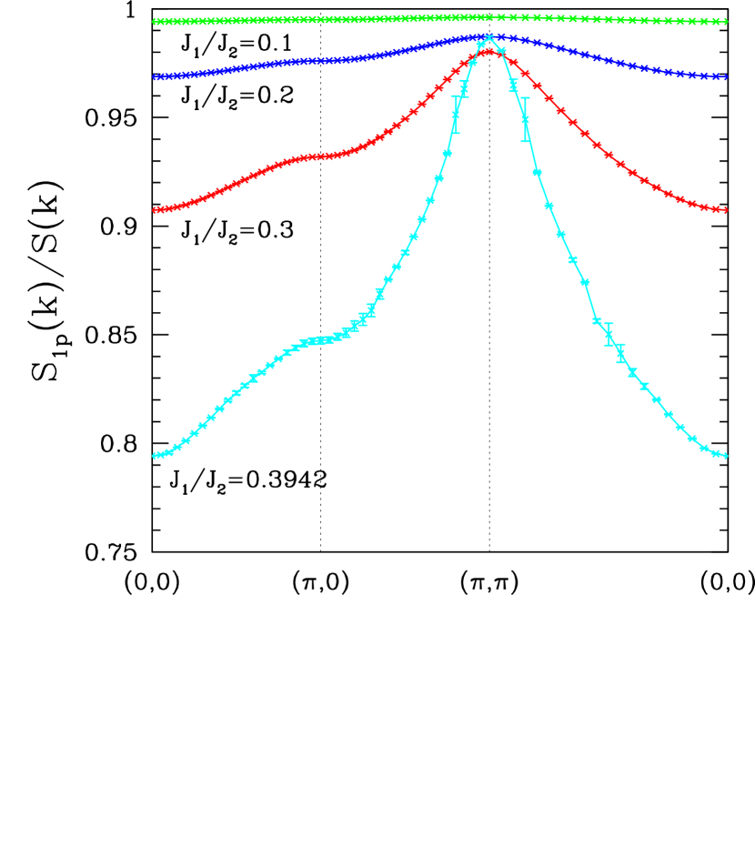
Figure 10: [Color online] The ratio $S_{1p}({\bf k})/S({\bf k})$ of the 1-particle static structure factor to the total static structure factor as a function of ${\bf k}$, for various couplings $\lambda=J_{1}/J_{2}$.

Further information may be obtained from the series for $S({\bf k})$ and $S_{1p}({\bf k})$ at the Néel momentum $(\pi,\pi)$, which are given in Table I. A Dlog Padé analysis of these series, biased at $\lambda_{c}=0.3942$, shows both $S({\bf k})$ and $S_{1p}({\bf k})$ diverging as $\lambda\rightarrow\lambda_{c}$ with exponents $-0.68(1)$ and $-0.69(1)$ respectively. The series for the ratio $S_{1p}/S$ shows no sign of a singularity at this point, remaining almost constant, within 2% of unity at all couplings. This behaviour is quite different from the AHC case affleck1998 , where the ratio vanishes logarithmically at the critical point.

These results should be compared with theoretical expectations. From scaling theory (see Appendix B), the 1-particle structure factor in the vicinity of the critical point $S_{1p}(\pi,\pi)$ should scale like $(\lambda_{c}-\lambda)^{(\eta-1)\nu}$, at the critical (Néel) momentum. For the total structure factor at this point, scaling theory gives exactly the same exponent (see Appendix B). We expect this transition to belong to the universality class of the O(3) model in 3 dimensions, which has critical exponents guida1998 $\nu=0.707(4)$, $\eta=0.036(3)$, hence we expect $(\eta-1)\nu=-0.682(5)$, which is quite compatible with the numerical estimates obtained above.

How does $S_{1p}$ behave at the critical coupling away from the Néel momentum? In the transverse Ising model hamer2006 , it was found that the 1-particle residue function $A({\bf k})$ (see Appendix B) vanishes like $(\lambda_{c}-\lambda)^{\eta\nu}$ at all momenta, with a small exponent $\eta\nu=+0.025(3)$, so that $S_{1p}$ vanishes in the same fashion as $\lambda\rightarrow\lambda_{c}$. Does the same thing happen in the present case? This is by no means obvious in Figure 10, which shows the ratio $S_{1p}/S$ dropping slowly as $\lambda$ increases, but nowhere near zero.

Table 2: Series coefficients of $\lambda^{N}$ for the binding energies in the channels $S=0,1$, and antibinding energy (S = 2). The $S=0$ and $S=2$ states are doubly degenerate.

N	S = 0	S = 1	S = 1	S = 2
0	0.00000000000000D+00	0.00000000000000D+00	0.00000000000000D+00	0.00000000000000D+00
1	1.00000000000000D+00	5.00000000000000D-01	5.00000000000000D-01	5.00000000000000D-00
2	-2.25000000000000D+00	-2.12500000000000D+00	-3.12500000000000D+00	-1.37500000000000D+00
3	-1.93750000000000D+00	1.31250000000000D+00	-2.93750000000000D+00	1.87500000000000D-01
4	-3.07812500000000D+00	2.97656250000002D+00	-2.77343749999998D+00	2.27343750000000D+00
5	3.47656250000001D-01	1.07812500000003D+00	3.06250000000002D+00	2.36718750000000D+00
6	-9.69726562500059D-01	-1.00527343749999D+01	8.35742187500014D+00	-8.13476562500000D+00
7	3.51385498046887D+00	7.44207763671879D+00	4.07301635742189D+01	-7.26873779296875D+00
8		7.92327880859462D+00	1.69468475341798D+02	-3.48072814941411D+00

To pursue this question further, we have studied the series at ${\bf k}=(0,0)$, also given in Table I. A Dlog Padé analysis of these series reveals a dominant singularity at $\lambda=-0.43(1)$, with exponent around $-0.65(3)$ in both cases. This will correspond to another critical point of the model, where the spins order ferromagnetically in the planes, and antiferromagnetically between them. At positive $\lambda$, there is no sign of a pole around $\lambda=0.4$. The ratio $S_{1p}/S$ decreases smoothly to around $0.80$ at the critical coupling, and shows no sign of vanishing there. Thus it appears that in this case the renormalized residue function does not vanish at $\lambda_{c}$, except at the Néel momentum.

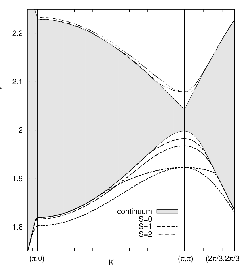
Figure 11: Series estimates of the energies of 2-particle states at fixed $\lambda=0.1$, along symmetry lines in the Brillouin zone.

III.2 Two-particle excitations

We have generalized the computer codes which were previously used to calculate 2-particle perturbation series for 1-dimensional models trebst2000 to cover the two-dimensional case. Figure 11 shows the dispersion diagram estimated from the perturbation series for 2-particle states at $\lambda=0.1$. We have zoomed in on the region where the bound states occur. It can be seen that S = 0 singlet and S = 1 triplet bound states emerge below the continuum near ${\bf k}=(\pi,\pi)$, and S = 2 quintuplet antibound states appear above the continuum, as predicted by the triplet-wave theory. The $S=0$ and $S=2$ states are doubly degenerate at ${\bf k}=(\pi,\pi)$. All states merge with the continuum at some finite momentum point ${\bf k}$, and for the most part they appear to merge at a tangent, as in the one-dimensional case zheng2001 . The results look very similar to the triplet-wave predictions shown in Figure 8.

Figure 12 shows the behaviour of the binding energies at ${\bf k}=(\pi,\pi)$ as functions of $\lambda$, as estimated from Padé approximants to the series given in Table 2. The degenerate pair of singlet bound states are the lowest over most of the range, but merge back into the continuum somewhat before the critical point. One of the triplet states disappears into the continuum quite early, but the other appears to disappear only at the critical point. For the AHC, the binding energies also vanished at the critical endpoint of the dimerized phase. The pair of antibound quintuplet states, on the other hand, appear to remain above the continuum even at the critical point, from our estimates.

Figure 12: Binding energies as functions of $\lambda$, relative to the 2-particle continuum. For bound states, we graph $(E_{2p}-E^{-}_{cont})$, while for antibound states we graph $(E_{2p}-E^{+}_{cont})$, where $E^{\pm}_{cont}$ denote the upper/lower bounds of the continuum.

IV Summary and Conclusions

In this paper, we have used a modified triplet-wave theory and dimer series expansions to study the Heisenberg bilayer system in the dimerized phase. As found in earlier papers hida1992 ; zheng1997 ; sandvik1994 , the model displays a quantum phase transition from the dimerized phase to a Néel phase at a coupling ratio $\lambda_{c}=0.394(1)$, with critical indices in good agreement with the predicted values from the classical O(3) nonlinear sigma model in three dimensions, $\nu=0.707$ and $\eta=0.036$.

Our modified triplet-wave approach is found to give good results at small couplings $\lambda$, but towards the critical region the self-consistent Born approximation approach of Kotov et al. kotov1998 ; shevchenko1999 , which includes some important higher-order terms, gives much better results. The triplet-wave approach predicts, as for other dimerized systems, two-particle bound states in the $S=0$ and $S=1$ channels where an antiferromagnetic alignment of spins can give rise to an attractive force, and antibound states in the $S=2$ channel, where the spin alignment is necessarily ferromagnetic and repulsive.

Our series calculations focused upon two major features, the critical behaviour of the static transverse structure factor, and the spectrum of 2-particle bound states in the model. The integrated structure factor $S({\bf k})$ and the single-particle component $S_{1p}({\bf k})$ were both found to diverge at the critical point for momentum ${\bf k}=(\pi,\pi)$, with exponents agreeing well with the predicted value $(\eta-1)\nu=-0.68$. The ratio $S_{1p}/S$ remains finite throughout the region, even at the critical coupling $\lambda_{c}$. This is in contrast to the case of the alternating Heisenberg chain, where the 1-particle component vanishes logarithmically at the critical point affleck1998 ; hamer2003 . In fact, here the one-particle state dominates everywhere ($S_{1p}/S\geq 80\%$).

In the 2-particle sector, a pair of bound states is found in the $S=0$ and $S=1$ channels near momentum ${\bf k}=(\pi,\pi)$, as predicted, and a pair of antibound states in the $S=2$ channel, the pairing being a two-dimensional effect. The singlet $S=0$ states have the lowest energies at small couplings, but both $S=0$ states and one $S=1$ state merge back into the continuum as $\lambda$ increases, leaving only one remaining triplet bound state, which appears to merge with the continuum right at $\lambda=\lambda_{c}$. In the S=2 channel, both antibound states appear to remain above the 2-particle continnum at all couplings $\lambda>0$.

As one moves away from ${\bf k}=(\pi,\pi)$, the bound/antibound states eventually merge into the continuum also. They appear to merge with the continuum at a tangent, much as in the one-dimensional case hamer2003 .

In future work, we hope to perform similar calculations for other two-dimensional models, such as the simple Heisenberg model on the square lattice, and the Shastry-Sutherland model, which has already been studied by Knetter et al. knetter2000 , and where the two-particle states display some intriguing behaviour.

$$\Phi^{(1)}_{4}(1234) = \frac{1}{4}[(\gamma_{1}+\gamma_{2})(c_{1}c_{2}+c_{1}s_{2}+s_{1}c_{2}+s_{1}s_{2})(c_{3}s_{4}+s_{3}c_{4})+(\gamma_{3}+\gamma_{4})(s_{1}c_{2}+c_{1}s_{2})(c_{3}c_{4}+c_{3}s_{4}+s_{3}c_{4}+s_{3}s_{4})$$ (63)

$$+\gamma_{{\bf 1+3}}(c_{1}s_{3}-s_{1}c_{3})(c_{2}s_{4}-s_{2}c_{4})+\gamma_{{\bf 1+4}}(c_{1}s_{4}-s_{1}c_{4})(c_{2}s_{3}-s_{2}c_{3})]$$

$$\Phi^{(2)}_{4}(1234) = \frac{1}{2}[(\gamma_{1}+\gamma_{2})(s_{3}c_{4}+c_{3}s_{4})(c_{1}c_{2}+c_{1}s_{2}+s_{1}c_{2}+s_{1}s_{2})+(\gamma_{3}+\gamma_{4})(c_{1}s_{2}+s_{1}c_{2})(c_{3}c_{4}+c_{3}s_{4}+s_{3}c_{4}+s_{3}s_{4})$$ (64)

$$+\gamma_{{\bf 1-4}}(c_{1}c_{4}-s_{1}s_{4})(c_{2}c_{3}-s_{2}s_{3})+\gamma_{{\bf 1-3}}(c_{1}c_{3}-s_{1}s_{3})(c_{2}c_{4}-s_{2}s_{4})]$$

$$\Phi^{(3)}_{4}(1234) = (\gamma_{1}+\gamma_{3})(c_{1}c_{3}+c_{1}s_{3}+s_{1}c_{3}+s_{1}s_{3})(c_{2}c_{4}+s_{2}s_{4})+(\gamma_{2}+\gamma_{4})(c_{2}c_{4}+c_{2}s_{4}+s_{2}c_{4}+s_{2}s_{4})(c_{1}c_{3}+s_{1}s_{3})$$ (65)

$$+\gamma_{{\bf 1-4}}(c_{1}c_{4}-s_{1}s_{4})(s_{2}s_{3}-c_{2}c_{3})+\gamma_{{\bf 1+2}}(c_{1}s_{2}-s_{1}c_{2})(s_{3}c_{4}-c_{3}s_{4})$$

$$\Phi^{(4)}_{4}(1234) = (\gamma_{1}+\gamma_{2})(c_{1}c_{2}+c_{1}s_{2}+s_{1}c_{2}+s_{1}s_{2})(c_{3}c_{4}+s_{3}s_{4})+(\gamma_{3}+\gamma_{4})(c_{1}s_{2}+s_{1}c_{2})(c_{3}c_{4}+c_{3}s_{4}+s_{3}c_{4}+s_{3}s_{4})$$ (66)

$$+\gamma_{{\bf 1-4}}(c_{1}c_{4}-s_{1}s_{4})(c_{2}s_{3}-s_{2}c_{3})+\gamma_{{\bf 1+3}}(c_{2}c_{4}-s_{2}s_{4})(c_{1}s_{3}-s_{1}c_{3})$$

We have ‘symmetrized’ these expressions with respect to their indices, using momentum conservation.

APPENDIX B. Scaling Theory for Structure Factors

Let us briefly review scaling theory in the vicinity of a quantum critical point for quantum spin models on a lattice. Firstly, the integrated or static structure factor marshall1971 ; oitmaa2006

$$S^{\alpha\beta}({\bf k})=\frac{1}{N}\sum_{i,j}e^{i{\bf k\cdot(r_{i}-r_{j})}}<S^{\alpha}_{j}S^{\beta}_{i}>_{0}$$ (67)

is just the Fourier transform of the spin correlation function in the ground state, where $S^{\alpha}_{j}$ represents the $\alpha$ component of the spin operator at site $j$. In the continuum approximation near the critical point, this reduces to

$$S^{\alpha\beta}({\bf k})=\int d^{n}\ re^{i{\bf k\cdot r}}<S^{\alpha}({\bf r})S^{\beta}(0)>_{0}$$ (68)

where $n$ is the number of spatial dimensions.

The oscillating factor $\exp(i{\bf k\cdot r})$ will kill off the contributions from large distances unless it is compensated by a corresponding oscillation $\exp(-i{\bf k_{0}\cdot r})$ in the correlation function. Then we can write

$$S^{\alpha\beta}({\bf k})=\int d^{n}r\ e^{i{\bf q\cdot r}}g(r)$$ (69)

where ${\bf q}={\bf k-k_{0}}$, and g(r) is a smooth function. Scaling theory cardy1996 then tells us that in the vicinity of the critical point

$$g(r)\sim r^{-(d-2+\eta)}f(r/\xi)$$ (70)

where $d=n+1$ is the number of space-time dimensions, and $\xi$ is the correlation length. Thus when ${\bf k}={\bf k_{0}}$, the ‘critical momentum’, we have

$$S^{\alpha\beta}({\bf k_{0}}) = \int d^{d-1}r\ r^{-(d-2+\eta)}f(r/\xi)$$ (71)

$$\sim \xi^{1-\eta}\int_{0}^{\infty}d^{d-1}z\ z^{-(d-2+\eta)}f(z)$$

where $z=r/\xi$. As the coupling $\lambda\rightarrow\lambda_{c}$, corresponding to a quantum phase transition, we expect

$$\xi\sim(\lambda_{c}-\lambda)^{-\nu}$$ (72)

and hence

$$S^{\alpha\beta}({\bf k_{0}})\sim(\lambda_{c}-\lambda)^{-(1-\eta)\nu},$$ (73)

as noted in the text.

For ${\bf q}$ small but non-zero, $|{\bf q}|\ll 1/\xi$, we have

$$S^{\alpha\beta}({\bf k}) \sim \xi^{1-\eta}\int_{0}^{\infty}d^{d-1}z\ z^{-(d-2+\eta)}e^{iqz\xi\cos(\theta)}f(z)$$

$$\sim q^{-(1-\eta)}\int_{0}^{\infty}d^{d-1}z^{\prime}\ z^{\prime-(d-2+\eta)}e^{iz^{\prime}\cos(\theta)}f^{\prime}(z^{\prime})$$

so that at the critical coupling we expect $S^{\alpha\beta}({\bf k})$ to scale like $q^{-(1-\eta)}$ at small $q$.

For the 1-particle structure factor, we may paraphrase Sachdev’s argument sachdev1999 as follows. Assuming relativistic invariance of the effective field theory, which applies to many though not all models, the dynamic susceptibility in the vicinity of a quasiparticle pole is expected to have the form

$$\chi({\bf k},\omega) = \frac{A}{c^{2}{\bf k}^{2}+\Delta^{2}-(\omega+i\epsilon)^{2}}+\cdots$$ (75)

where $\epsilon$ is a positive infinitesimal, $c$ the quasiparticle velocity, $\Delta$ is the quasiparticle energy gap, and $A$ is the “quasiparticle residue”. Then the dynamic structure factor is

$$S({\bf k},\omega) = \frac{1}{\pi}Im\{\chi({\bf k},\omega\}$$ (76)

Let

$$E({\bf k}) = \sqrt{c^{2}{\bf k}^{2}+\Delta^{2}}$$ (77)

then from (75), (76) and (77) we can write the dynamic structure factor for the 1-particle state

$$S_{\rm 1p}({\bf k},\omega) = \frac{A({\bf k})}{2E({\bf k})}\delta(\omega-E({\bf k}))$$ (78)

and hence the static structure factor

$$S_{\rm 1p}({\bf k}) = \int_{-\infty}^{\infty}d\omega S_{1p}({\bf k},\omega)=\frac{A({\bf k})}{2E({\bf k})}$$ (79)

where $A({\bf k})$ is the residue function.

From renormalization group theory cardy1996 , the scaling dimensions of these quantities are expected to be hamer2006 ${\rm dim}[\chi]=-2+\eta$ and ${\rm dim}[A]=\eta$, or in other words we expect near the critical point

$$A({\bf k}_{0}) \sim (\lambda_{c}-\lambda)^{\eta\nu},$$

$$E({\bf k_{0}}) \sim (\lambda_{c}-\lambda)^{\nu},$$ (80)

and hence

$$S_{1p}({\bf k_{0}}) \sim (\lambda_{c}-\lambda)^{-(1-\eta)\nu},$$ (81)

just as for the total structure factor. This is the result quoted in the text.

References

• (1) D.A. Tennant, C. Broholm, D.H. Reich, S.E. Nagler, G.E. Granroth, T. Barnes, K. Damle, G. Xu, Y. Chen and B.C. Sales, Phys. Rev. B67, 054414 (2003).
• (2) J. Oitmaa, C.J. Hamer and W. Zheng, Series Expansion Methods for Strongly Interacting Lattice Models (Cambridge University Press, 2006).
• (3) S.Trebst, H. Monien, C.J. Hamer, W-H Zheng and R.R.P. Singh, Phys. Rev. Let.t 85, 4373 (2000); W-H Zheng, C.J. Hamer, R.R.P. Singh, S. Trebst and H. Monien, Phys. Rev. B63, 144411 (2001).
• (4) See for example C. Knetter, A. Buehler, E. Mueller-Hartmann and G.S. Uhrig, Phys. Rev. Lett. 85, 3958 (2000).
• (5) D.Reznik et al., Phys. Rev. B53, R14741 (1996).
• (6) S.M. Hayden, G. Aeppli, T.G. Perring, H.A. Mook and F. Dogan, Phys. Rev. B54, R6905 (1996).
• (7) A.J. Millis and H. Monien, Phys. Rev. B54, 16172 (1996).
• (8) S. PailhΓ¨s, C. Ulrich, B. FauquΓ©, V. Hinkov, Y. Sidis, A. Ivanov, C.T. Lin, B. Keimer and P. Bourges, Phys. Rev. Lett. 96, 257001 (2006).
• (9) M.B. Stone, C. Broholm, D.H. Reich, O. Tchernyshyov, P. Vorderwisch and N. Harrison, Phys. Rev. Lett. 96, 257203 (2006).
• (10) T. Sommer, M. Vojta and K.W. Becker, Eur. Phys. J. B23, 329 (2001).
• (11) A.W. Sandvik, Phys. Rev. Lett. 89, 177201 (2002).
• (12) T. Zhou, Z.D. Wang and J-X. Li, Phys. Rev. B75, 024516 (2007).
• (13) R. Sknepnek, T. Vojta and M. Vojta, Phys. Rev. Lett. 93, 097201 (2004).
• (14) K. Hida, J. Phys. Soc. Jpn. 61, 1013 (1992).
• (15) W-H. Zheng, Phys. Rev. B55, 12267 (1997).
• (16) M.P. Gelfand, Phys. Rev. B53, 11309 (1996).
• (17) A.W. Sandvik and D.J. Scalapino, Phys. Rev. Lett. 72, 2777 (1994).
• (18) A.W. Sandvik, A.V. Chubukov and S. Sachdev, Phys. Rev. B51, 16483 (1995).
• (19) A.W. Sandvik and D.J. Scalapino, Phys. Rev. B53, R526 (1996).
• (20) A.J. Millis and H. Monien, Phys. Rev. Lett. 70, 2810 (1993); Phys. Rev. B50, 16606 (1994).
• (21) T. Miyazaki, I. Nakamura and D. Yoshioka, Phys. Rev. B53, 12206 (1996).
• (22) T. Matsuda and K. Hida, J. Phys. Soc Jpn. 59, 2223 (1990); K. Hida, ibid 59, 2230 (1990).
• (23) A.V. Chubukov and D.K. Morr, Phys. Rev. B52, 3521 (1995).
• (24) P.V. Shevchenko and O.P. Sushkov, Phys. Rev. B59, 8383 (1999).
• (25) V.N. Kotov, O.P. Sushkov, W-H. Zheng and J. Oitmaa, Phys. Rev. Letts. 80, 5790 (1998).
• (26) S. Sachdev and R.N. Bhatt, Phys. Rev. B41, 9323 (1990).
• (27) A. Collins, C.J. Hamer and W-H Zheng, Phys. Rev. B74, 144414 (2006); ibid. B75, 139902(E) (2007).
• (28) I.G. Gochev, Phys. Rev. B49, 9594 (1994).
• (29) G.S. Uhrig and H.J. Schulz, Phys. Rev. B54, R9624 (1996).
• (30) R.R.P. Singh, M.P. Gelfand and D.A. Huse, Phys. Rev. Lett. 61, 2484 (1988).
• (31) C.J. Hamer, W. Zheng and R.R.P. Singh, Phys. Rev. B68, 214408 (2003).
• (32) R. Guida and J. Zinn-Justin, J. Phys. A31, 8103 (1998).
• (33) C.J. Hamer, J. Oitmaa and W. Zheng, Phys. Rev. B74, 174428 (2006).
• (34) W-H. Zheng, C.J. Hamer, R.R.P. Singh, S. Trebst and H. Monien, Phys. Rev. B63, 144411 (2001).
• (35) I. Affleck, J. Phys. A31, 4573 (1998).
• (36) S. Sachdev, Quantum Phase Transitions (Cambridge University Press, Cambridge, U.K., 1999).
• (37) W. Marshall and S.W. Lovesey, Theory of Thermal Neutron Scattering, The International Series of Monographs on Physics (Oxford, Clarendon Press, 1971).
• (38) J. Cardy, Scaling and Renormalization in Statistical Physics (Cambridge 1996).