Ricci Flow and Entropy Model for Avascular Tumor Growth and Decay Control

Abstract

Prediction and control of cancer invasion is a vital problem in medical science. This paper proposes a modern geometric Ricci–flow and entropy based model for control of avascular multicellular tumor spheroid growth and decay. As a tumor growth/decay control tool, a monoclonal antibody therapy is proposed.

Keywords: avascular tumor growth and decay, multicellular tumor spheroid, Ricci flow and entropy, nonlinear heat equation, monoclonal antibody cancer therapy

1 Introduction

Cancer is one of the main causes of morbidity and mortality in the world. There are several different stages in the growth of a tumor before it becomes so large that it causes the patient to die or reduces permanently their quality of life. Developed countries are investing large sums of money into cancer research in order to find cures and improve existing treatments. In comparison to molecular biology, cell biology, and drug delivery research, mathematics has so far contributed relatively little to the area [1].

On the other hand, consider the vital problem of prediction and control/prevention of some natural disaster (e.g., a hurricane). The role of science in dealing with a phenomenon/treat like this can be depicted as the following OUPC feedback–loop (see [2]):

$$\begin{array}[]{ccccccc}Observation&\longrightarrow&Understanding&\longrightarrow&Prediction&\longrightarrow&Control\\ \uparrow&&&&&&\downarrow\\ &\longleftarrow&\longleftarrow&\longleftarrow&\longleftarrow&\longleftarrow\end{array}$$

with the following four components/phases:

1. $Observation$, i.e., monitoring a phenomenon in case, using experimental sensing/measuring methods (e.g., orbital satellite imaging). This phase produces measurement data that could be fitted as graphs of analytical functions.

2. $Understanding$, in the form of geometric pattern recognition, i.e., recognizing the turbulent patterns of spatio–temporal chaotic behavior of the approaching hurricane, in terms of geometric objects (e.g., tensor– and spinor–fields). This phase recognizes the observation graphs as cross–sections of some jet bundles, thus representing the validity criterion for the observation phase.

3. $Prediction$: when, where and how will the hurricane strike?
   Now, common, inductive approach here means fitting a statistical model into empirical satellite data. However, we know that this works only for a very short time in the future, as extrapolation is not a valid predictive procedure, even if (adaptive) extended Kalman filter is used. Instead, we suggest a deductive approach of fitting some data into a well–defined dynamical model. This means formulating a dynamical system on configuration and phase–space manifolds, which incorporates all previously recognized turbulent patterns of the hurricane’s spatio–temporal behavior. Once a valid dynamical model is formulated, the necessary empirical satellite data would include system parameters, initial and boundary conditions. So, this would be a pattern–driven modelling of the hurricane, rather than blind data–driven statistical modelling. This phase is the validity criterion for the understanding phase.

4. $Control$: this is the final stage of manipulating the hurricane to prevent the destruction. If we have already formulated a valid geometric–pattern–based dynamical model, this task can be relatively easily accomplished, as

   $$Control\;System\;=\;Dynamical\;System\;+\;Controller.$$

   So, here the problem is to design a feedback controller/compensator for the dynamical model. This phase is the validity criterion for the prediction phase.

Since there are three distinct stages to cancer development: avascular, vascular, and metastatic – researchers often concentrate their efforts on answering specific OUPC–related questions on each of these stages (see [3]). In particular, as some tumor cell lines grown in vitro form 3–dimensional (3D, for short) spherical aggregates, the relative cheapness and ease of in vitro experiments in comparison to animal experiments has made 3D multicellular tumor spheroids (MTS, see Figure 1, as well as e.g., Figure 6 in [3]) very popular in vitro model system of avascular tumors [4]. They are used to study how local micro-environments affect cellular growth/decay, viability, and therapeutic response (see [5]). MTS are often combined with 3D medical imaging [9], 4D confocal imaging [10], 3D video holography through living tissue [11] and 3D metabolic imaging imaging bioluminescence [6]. MTS provide, allowing strictly controlled nutritional and mechanical conditions, excellent experimental patterns to test the validity of the proposed mathematical models of tumor growth/decay [8].

Figure 1: An example of multicellular tumor spheroid (MTS): a differential interference contrast image.

A number of mathematical models of avascular tumor growth inside the MTS were reviewed in [3]. These were generally divided into continuum cell population models described by diffusion partial differential equations (PDEs) of continuum mechanics [2, 16] combined with chemical kinetics, and discrete cell population models described by ordinary differential equations (ODEs). Besides, in many cell population models it is possible to empirically demonstrate the presence of attractors that operate starting from different initial conditions [12, 13].

A general model of multi–phase tumor growth (inside the MTS) is given in [3] by the parabolic reaction–diffusion PDE,

$$\partial_{t}\Phi_{i}=\nabla\cdot(D_{i}\Phi_{i})-\nabla\cdot(\mathbf{v}_{i}\Phi_{i})+\lambda_{i}(\Phi_{i},C_{i})-\mu_{i}(\Phi_{i},C_{i})$$ (1)

($\partial_{t}\equiv\partial/\partial{t}$), where for phase $i$, $\Phi_{i}$ is the volume fraction ($\sum_{i}\Phi_{i}=1$), $D_{i}$ is the random motility or diffusion, $\lambda_{i}(\Phi_{i},C_{i})$ is the chemical and phase dependent production, and $\mu_{i}(\Phi_{i},C_{i})$ is the chemical and phase dependent degradation/death, and $\mathbf{v}_{i}$ is the cell velocity defined by the constitutive equation

$$\mathbf{v}_{i}=-\mu\nabla p,$$ (2)

where $\mu$ is a positive constant describing the viscous–like properties of tumor cells and $p$ is the spheroid internal pressure.

In particular, the multi-phase equation (1) splits into two heat–like mass–conservation PDEs [3],

$$\partial_{t}\Phi^{C}=S^{C}-\nabla\cdot(\mathbf{v}^{C}\Phi^{C}),\qquad\partial_{t}\Phi^{F}=S^{F}-\nabla\cdot(\mathbf{v}^{F}\Phi^{F}),$$ (3)

where $\Phi^{C}$ and $\Phi^{F}$ are the tissue cell/matrix and fluid volume fractions, respectively, $\mathbf{v}^{C}$ and $\mathbf{v}^{F}$ are the cell/matrix and the fluid velocities (both defined by their constitutive equations of the form of (2)), $S^{C}$ is the rate of production of solid phase tumor tissue and $S^{F}$ is the creation/degradation of the fluid phase. Conservation of matter in the tissue, $\Phi^{C}+\Phi^{F}=1$, implies that $\nabla\cdot$($\mathbf{v}^{C}\Phi^{C}$ +$\mathbf{v}^{F}\Phi^{F}$) = $\Phi^{C}+\Phi^{F}$. The assumption that the tumor may be described by two phases only implies that the new cell/matrix phase is formed from the fluid phase and vice versa, so that $S^{C}+S^{F}=0$. The detailed biochemistry of tumor growth can be coupled into the model above through the growth term $S^{C}$, with equations added for nutrient diffusion, see [3] and references therein.

The multi-phase tumor growth model (1) has been derived from the classical transport/mass conservation equations for different chemical species inside the MTS [3],

$$\partial_{t}C_{i}=P_{i}-\nabla\cdot\mathbf{N}_{i}.$$ (4)

Here $C_{i}$ are the concentrations of the chemical species, subindex $a$ for oxygen, $b$ for glucose, $c$ for lactate ion, $d$ for carbon dioxide, $e$ for bicarbonate ion, $f$ for chloride ion, and $g$ for hydrogen ion concentration; $P_{i}$ is the net rate of consumption/production of the chemical species both by tumor cells and due to the chemical reactions with other species; and $\mathbf{N}_{i}$ is the flux of each of the chemical species inside the tumor spheroid, given (in the simplest case of uncharged molecules of glucose, $O_{2}$ and $CO_{2}$) by Fick’s law,

$$\mathbf{N}_{i}=-D_{i}\nabla C_{i},$$

where $D_{i}$ are (positive) constant diffusion coefficients. In case of charged molecules of ionic species, the flux $\mathbf{N}_{i}$ contains also the (negative) gradient of the volume fractions $\Phi_{i}$.

In all above cases, tumor growth is, in terms of statistical mechanics, associated to entropy growth. The more uncertainty (measured as a number of tumor microstates) the tumor spheroid possesses, the larger is its entropy. Formally, we can apply Shannon formula to the probability distributions $(p_{1},\cdots,p_{n})$ of cancer cells within the body,

$$S(p_{1},\cdots,p_{n})~{}=~{}-\sum_{i}p_{i}\log_{2}p_{i}.$$

In other words, if we do not control the tumor growth, naturally it is governed by the Second Law of Thermodynamics:

$$\partial_{t}S~{}\geq~{}0,$$

which is an expression of the universal law of increasing entropy, stating that the entropy (i.e., total number of tumor cells) of an isolated thermodynamic system (i.e., human body) which is not in equilibrium will tend to increase over time, approaching a maximum value at equilibrium (i.e., death threatening situation).

On the other hand, the Ricci flow equation (or, the parabolic Einstein equation), introduced by R. Hamilton in 1982 [23], is the nonlinear heat–like evolution equation

$$\partial_{t}g_{ij}=-2R_{ij},$$ (5)

for a time–dependent Riemannian metric $g=g_{ij}(t)$ on a smooth real $n-$manifold $M$ with the Ricci curvature tensor $R_{ij}$. This equation roughly says that we can deform any metric on a 2D surface or $n$D manifold by the negative of its curvature; after normalization (see Figure 2), the final state of such deformation will be a metric with constant curvature. The factor of 2 in (5) is more or less arbitrary, but the negative sign is essential to insure a kind of complex volume exponential decay, since the Ricci flow equation (5) is a kind of nonlinear generalization of the standard linear heat equation

$$\partial_{t}u=\Delta u.$$ (6)

Like the heat equation (6), the Ricci flow equation (5) is well behaved in forward time and acts as a kind of smoothing operator (but is usually impossible to solve in backward time). If some parts of a solid object are hot and others are cold, then, under the heat equation, heat will flow from hot to cold, so that the object gradually attains a uniform temperature. To some extent the Ricci flow behaves similarly, so that the Ricci curvature ‘tries’ to become more uniform [24], thus depicting a monotonic entropy growth, $\partial_{t}S\geq 0$, which is due to the positive definiteness of the metric $g_{ij}\geq 0$, and naturally implying the arrow of time [20, 17, 16].

In a suitable local coordinate system, the Ricci flow equation (5) has a nonlinear heat–type form, as follows. At any time $t$, we can choose local harmonic coordinates so that the coordinate functions are locally defined harmonic functions in the metric $g(t)$. Then the Ricci flow takes the form (see e.g., [25])

$$\partial_{t}g_{ij}=\Delta g_{ij}+Q_{ij}(g,\partial g),$$ (7)

where $\Delta$ is the Laplace–Beltrami differential operator on functions with respect to the metric $g$ and $Q$ is a lower–order term quadratic in $g$ and its first order partial derivatives. From the analysis of nonlinear heat PDEs, one obtains existence and uniqueness of forward–time solutions to the Ricci flow (7) on some time interval, starting at any smooth initial metric $g_{0}=g_{ij}(0)$.

As a simple example of the Ricci flow equations (5)–(7), consider a round spherical boundary $S^{2}$ of the MTS of radius $r$. The metric tensor on $S^{2}$ takes the form

$$g_{ij}=r^{2}\hat{g}_{ij},$$

where $\hat{g}_{ij}$ is the metric for a unit sphere, while the Ricci tensor

$$R_{ij}=(n-1)\hat{g}_{ij}$$

is independent of $r$. The Ricci flow equation on $S^{2}$ reduces to

$$\dot{r}^{2}=-2(n-1),$$

with solution

$$r^{2}(t)=r^{2}(0)-2(n-1)t.$$

Thus the boundary sphere $S^{2}$ collapses to a point in finite time (see [24]).

More generally, the following geometrization conjecture holds for an MTS 3–manifold $M$: Suppose that we start with a compact initial MTS–manifold $M_{0}$ whose Ricci tensor $R_{ij}$ is everywhere positive definite. Then, as $M_{0}$ shrinks to a point under the Ricci flow (5), it becomes rounder and rounder. If we rescale the metric $g_{ij}$ on $M_{0}$ so that the volume of $M_{0}$ remains constant, then $M_{0}$ converges towards another compact MTS–manifold $M_{1}$ of constant positive curvature (see [23]).

In case of even more general MTS $3-$manifolds (outside the class of positive Ricci curvature metrics), the situation is much more complicated, as various singularities may arise. One way in which singularities may arise during the Ricci flow is that a spherical boundary $S^{2}=\partial M$ of an MTS $3-$manifold $M$ may collapse to a point in finite time. Such collapses can be eliminated by performing a kind of “geometric surgery” on the MTS manifold $M$, that is a sophisticated sequence of cutting and pasting without accumulation of time errors (see [22]). After a finite number of such surgeries, each component either: (i) converges towards a 3–manifold of constant positive Ricci curvature which shrinks to a point in finite time, or possibly (ii) converges towards an $S^{2}\times S^{1}$ which shrinks to a circle $S^{1}$ in finite time, or (iii) admits a “thin–thick” decomposition of [30]. Therefore, one can choose the surgery parameters so that there is a well defined Ricci-flow-with surgery, that exists for all time [22].

In this paper we use the evolving geometric machinery of the volume–decaying and entropy–growing Ricci flow $g(t)$, given by equations (5)–(7), for modelling general 3D avascular MTS decay, corresponding to parabolic multi–phase reaction–diffusion PDEs (1)–(4).

2 Ricci flow and multi-phase avascular MTS decay control

2.1 Geometrization Conjecture

Recall that geometry and topology of smooth surfaces are related by the Gauss–Bonnet formula for a closed surface $\Sigma$ (see, e.g., [2, 17])

$$\frac{1}{2\pi}\iint_{\Sigma}K\,dA=\chi(\Sigma)=2-2\,{\mathrm{g}en}(\Sigma),$$ (8)

where $dA$ is the area element of a metric $g$ on $\Sigma$, $K$ is the Gaussian curvature, $\chi(\Sigma)$ is the Euler characteristic of $\Sigma$ and ${\mathrm{g}en}(\Sigma)$ is its genus, or number of handles, of $\Sigma$. Every closed surface $\Sigma$ admits a metric of constant Gaussian curvature $K=+1,\,0$, or $-1$ and so is uniformized by elliptic, Euclidean, or hyperbolic geometry, which respectively have ${\mathrm{g}en}(S^{2})=0$ (sphere), ${\mathrm{g}en}(T^{2})=1$ (torus) and ${\mathrm{g}en}(\Sigma)>1$ (torus with several holes). The integral (8) is a topological invariant of the surface $\Sigma$, always equal to 2 for all topological spheres $S^{2}$ (that is, for all closed surfaces without holes that can be continuously deformed from the geometrical sphere) and always equal to 0 for the topological torus $T^{2}$ (i.e., for all closed surfaces with one hole or handle).

The general topological framework for the Ricci flow (5) is Thurston’s Geometrization Conjecture [30], which states that the interior of any compact 3–manifold can be split in an essentially unique way by disjoint embedded 2D spheres $S^{2}$ and tori $T^{2}$ into pieces and each piece admits one of 8 geometric structures (including (i) the 3D sphere $S^{3}$ with constant curvature $+1$; (ii) the 3D Euclidean space $\mathbb{R}^{3}$ with constant curvature 0 and (iii) the 3D hyperbolic space $\mathbb{H}^{3}$ with constant curvature $-1$). The geometrization conjecture (which has the Poincaré Conjecture as a special case) would give us a link between the geometry and topology of MTS 3–manifolds, analogous in spirit to the case of 2D surfaces.

In higher dimensions, the Gaussian curvature $K$ corresponds to the Riemann curvature tensor $\mathfrak{Rm}$ on a smooth $n-$manifold $M$, which is in local coordinates on $M$ denoted by its $(4,0)-$components $R_{ijkl}$, or its $(3,1)-$components $R_{ijk}^{l}$ (see Appendix, as well as e.g., [2, 17]). The trace (or, contraction) of $\mathfrak{Rm}$, using the inverse metric tensor $g^{ij}=(g_{ij})^{-1}$, is the Ricci tensor $\mathfrak{Rc}$, the 3D curvature tensor, which is in a local coordinate system $\{x^{i}\}_{i=1}^{n}$ defined in an open set $U\subset M$, given by

$$R_{ij}=\mathrm{tr}(\mathfrak{Rm})=g^{kl}R_{ijkl}$$

(using Einstein’s summation convention), while the scalar curvature is now given by the second contraction of $\mathfrak{Rm}$ as

$$R=\mathrm{tr}(\mathfrak{Rc})=g^{ij}R_{ij}.$$

In general, the Ricci flow $g_{ij}(t)$ is a one–parameter family of Riemannian metrics on a compact $n-$manifold $M$ governed by the equation (5), which has a unique solution for a short time for an arbitrary smooth metric $g_{ij}$ on $M$ [23]. If $\mathfrak{Rc}>0$ at any local point $x=\{x^{i}\}$ on $M$, then the Ricci flow (5) contracts the metric $g_{ij}(t)$ near $x$, to the future, while if $\mathfrak{Rc}<0$, then the flow (5) expands $g_{ij}(t)$ near $x$. The solution metric $g_{ij}(t)$ of the Ricci flow equation (5) shrinks in positive Ricci curvature direction while it expands in the negative Ricci curvature direction, because of the minus sign in the front of the Ricci tensor $R_{ij}$. In particular, in 2D, on a sphere $S^{2}$, any metric of positive Gaussian curvature will shrink to a point in finite time. At a general point, there will be directions of positive and negative Ricci curvature along which the metric will locally contract or expand (see [25]). In 3D, if a simply-connected compact 3–manifold $M$ has a Riemannian metric $g_{ij}$ with positive Ricci curvature then it is diffeomorphic to the 3–sphere $S^{3}$ [23].

All three Riemannian curvatures ($R,\mathfrak{Rc}$ and $\mathfrak{Rm}$), as well as the associated volume forms, evolve during the Ricci flow (5).

2.2 MTS evolution under the Ricci flow

The Ricci flow evolution equation (5) for the metric tensor $g_{ij}$ implies the evolution equation for the Riemann curvature tensor $\mathfrak{Rm}$,

$$\partial_{t}\mathfrak{Rm}=\triangle\mathfrak{Rm}+Q_{n},$$ (9)

where $Q_{n}$ is a certain quadratic expression of the Riemann curvatures. From the general $n-$curvature expression (9) we have two special cases important for MTS–evolution:

• The 3D evolution equation for the Ricci curvature tensor $\mathfrak{Rc}$ on an MTS 3–manifold $M$,

  $$\partial_{t}\mathfrak{Rc}=\triangle\mathfrak{Rc}+Q_{3},$$ (10)

  where $Q_{3}$ is a certain quadratic expression of the Ricci curvatures; and

• The 2D evolution equation for the scalar surface curvature $R$,

  $$\partial_{t}R=\triangle R+2|\mathfrak{Rc}|^{2},$$ (11)

  which holds both on an MTS 3–manifold $M$ and on its 2D boundary surface $\partial M$. Therefore, by the maximum principle, the minimum of $R$ is non–decreasing along the flow $g(t)$, both on $M$ and on $\partial M$ (see [21]).

Let us now see in detail how various MTS–related geometric quantities evolve given the short-time solution of the Ricci flow equation (5) on an MTS 3–manifold $M$. Let us first calculate the variation formulas for the Christoffel symbols and curvature tensors on $M$ and then the corresponding evolution equations (see [23, 31, 32]). If $g(s)$ is a one–parameter family of metrics on $M$ with

$$\partial_{s}g_{ij}=v_{ij},$$

then the variation of the Christoffel symbols $\Gamma_{ij}^{k}$ on $M$ is given by

$$\partial_{s}\Gamma_{ij}^{k}=\frac{1}{2}g^{kl}\left(\nabla_{i}v_{jl}+\nabla_{j}v_{il}-\nabla_{l}v_{ij}\right),$$ (12)

from which follows the evolution of the Christoffel symbols $\Gamma_{ij}^{k}$ under the Ricci flow $g(t)$ on $M$ given by (5),

$$\partial_{t}\Gamma_{ij}^{k}=-g^{kl}\left(\nabla_{i}R_{jl}+\nabla_{j}R_{il}-\nabla_{l}R_{ij}\right).$$

From (12) we calculate the variation of the Ricci tensor $R_{ij}$ on $M$ as

$$\partial_{s}R_{ij}=\nabla_{m}\left(\partial_{s}\Gamma_{ij}^{m}\right)-\nabla_{i}\left(\partial_{s}\Gamma_{mj}^{m}\right),$$ (13)

and the variation of scalar curvature $R$ on $M$ by

$$\partial_{s}R=-\Delta V+\mathrm{div}(\mathrm{div\,}v)-\left\langle v,\mathfrak{Rc}\right\rangle,$$ (14)

where $V=g^{ij}v_{ij}=\mathrm{tr}(v)$ is the trace of $v=(v_{ij})$.

If an MTS $3-$manifold $M$ is oriented, then the volume $3-$form on $M$ is given, in a positively oriented local coordinate system $\{x^{i}\}\in U\subset M$, by

$$d\mu=\sqrt{\det(g_{ij})}\,dx^{1}\wedge dx^{2}\wedge dx^{3}.$$ (15)

If $\partial_{s}g_{ij}=v_{ij},$ then

$$\partial_{s}d\mu=\frac{1}{2}Vd\mu.$$

The evolution of the volume form $d\mu$ under the Ricci flow $g(t)$ on $M$ is given by the exponential decay/growth relation with the scalar curvature $R$ as the rate constant,

$$\partial_{t}d\mu=-Rd\mu,$$ (16)

which gives an exponential decay for $R>0$ (elliptic geometry) and exponential growth for $R<0$ (hyperbolic geometry). The elementary volume evolution (16) implies the integral form of the exponential relation for the total MTS–volume

$$\mathrm{vol}(g)=\int_{M}d\mu,$$

in the form

$$\partial_{t}\mathrm{vol}(g(t))=-\int_{M}Rd\mu,$$

which again gives an exponential decay for elliptic $R>0$ and exponential growth for hyperbolic $R<0$.

This is a crucial point for the tumor decay control: we need to keep the elliptic geometry of the MTS – by all possible means. And naturally – it will be so, because it started as a spherical shape with $R>0$. We just need to keep the MTS in this shape and prevent any hyperbolic distortions of $R<0$. The, it will naturally have an exponential decay.

On the other hand, if we are not able to keep the positivity of the scalar curvature of the MTS, and thus prevent its expanding to in infinity (‘deadly’ hyperbolic case), we can also consider the normalized Ricci flow of the MTS on its 3–manifold $M$ (see Figure 2 as well as ref. [31]):

$$\partial_{t}\hat{g}_{ij}=-2\hat{R}_{ij}+\frac{2}{n}\hat{r}\hat{g}_{ij},$$ (17)

where

$$\hat{r}=\mathrm{vol}(\hat{g})^{-1}\int_{M}\hat{R}d\mu$$

is the average scalar curvature on $M$. We then have the MTS volume conservation law:

$$\partial_{t}\mathrm{vol}(\hat{g}(t))=0.$$

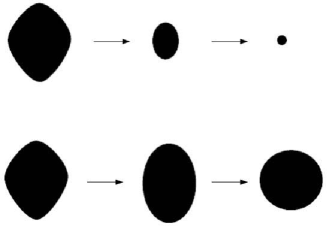
Figure 2: An example of Ricci flow normalization: unnormalized flow (up) and normalized flow (down).

To study the long–time existence of the normalized Ricci flow (17) on an MTS $3-$mani-fold $M$, it is important to know what kind of curvature conditions are preserved under the equation. In general, the Ricci flow $g(t)$ on $M$ tends to preserve some kind of positivity of curvatures. For example, positive scalar curvature $R$ is preserved both on $M$ and on its boundary $\partial M$. This follows from applying the maximum principle to the evolution equation (11) for scalar curvature $R$ both on $M$ and on $\partial M$. Also, positive Ricci curvature is preserved under the Ricci flow on $M$. (This is a special feature of 3D and is related to the fact that the Riemann curvature tensor may be recovered algebraically from the Ricci tensor and the metric in 3D [31].)

In particular, we have the following result (see [28]) for MTS–surfaces $\partial M$: Let $\partial M$ be a closed MTS–surface. Then for any initial 2D metric $g_{0}$ on $\partial M$, the solution to the normalized Ricci flow (17) on $\partial M$ exists for all time. Moreover, (i) If the Euler characteristic of $\partial M$ is non–positive, then the solution metric $g(t)$ on $\partial M$ converges to a constant curvature metric as $t\rightarrow\infty$; and (ii) If the scalar curvature $R$ of the initial metric $g_{0}$ is positive, then the solution metric $g(t)$ on $\partial M$ converges to a positive constant curvature metric as $t\rightarrow\infty.$ (For surfaces with non–positive Euler characteristic, the proof is based primarily on maximum principle estimates for the scalar curvature.)

In other words, the normalized Ricci flow of the MTS will make it completely round with a geometrical sphere shell – ideal for surgical removal. This is our second option for the MTS control. If we cannot force it to exponential decay, then we must try to normalize into a round spherical shell – which is suitable for surgical removal.

The negative flow of the total MTS–volume $\mathrm{vol}(g(t))$ is the Einstein–Hilbert functional, given by (see [43, 31, 25])

$$E(g)=\int_{M}Rd\mu=-\partial_{t}\mathrm{vol}(g(t)).$$

If we put $\partial_{s}g_{ij}=v_{ij},$ we have

$$\partial_{s}E(g) = \int_{M}\left(-\Delta V+\mathrm{div}(\mathrm{div\,}v)-\left\langle v,\mathfrak{Rc}\right\rangle+\frac{1}{2}RV\right)d\mu$$

$$= \int_{M}\left\langle v,\frac{1}{2}Rg_{ij}-R_{ij}\right\rangle d\mu,$$

so the critical points of $E(g)$ satisfy Einstein’s equation

$$\frac{1}{2}Rg_{ij}-R_{ij}=0.$$

The gradient flow of $E(g)$ on $M$, given by

$$\partial_{t}g_{ij}=2\left(\nabla E(g)\right)_{ij}=Rg_{ij}-2R_{ij},$$

is almost the Ricci flow (5). Thus, Einstein metrics are the fixed points of the Ricci flow $g(t)$ on $M$.

Let $\Delta$ denote the Laplacian acting on functions on an MTS $3-$mani-fold $M$, which is in local coordinates $\{x^{i}\}\in U\subset M$ given by

$$\Delta=g^{ij}\nabla_{i}\nabla_{j}=g^{ij}\left(\partial_{ij}-\Gamma_{ij}^{k}\partial_{k}\right).$$

For any smooth function $f$ on $M$ we have [23, 32]

$$\Delta\nabla_{i}f = \nabla_{i}\Delta f+R_{ij}\nabla_{j}f,\qquad\text{and}$$

$$\Delta|\nabla f|^{2} = 2|\nabla_{i}\nabla_{j}f|^{2}+2R_{ij}\nabla_{i}f\nabla_{j}f+2\nabla_{i}f\nabla_{i}\Delta f.$$

From this it follows that if we have

$$\mathfrak{Rc} \geq 0,\qquad\Delta f\equiv 0,\qquad|\nabla f|\equiv 1,\qquad\text{then}$$

$$\nabla\nabla f \equiv 0\qquad\text{and\qquad}\mathfrak{Rc}(\nabla f,\nabla f)\equiv 0.$$

Using $\Delta,$ we can write the linear heat equation on $M$ as

$$\partial_{t}u=\Delta u,$$

where $u$ is the MTS–temperature. In particular, the Laplacian acting on functions with respect to $g(t)$ will be denoted by $\Delta_{g(t)}$. If $(M,g(t))$ is a solution to the Ricci flow equation (5), then we have

$$\partial_{t}\Delta_{g(t)}=2R_{ij}\nabla_{i}\nabla_{j}.$$

Now, the evolution equation (11) for the scalar curvature $R$ under the Ricci flow (5) follows from (14). Using equation (27) from Appendix, we have:

$$\mathrm{div}(\mathfrak{Rc})=\frac{1}{2}\nabla R,\quad\text{so that}\quad\mathrm{div}(\mathrm{div}(\mathfrak{Rc}))=\frac{1}{2}\Delta R,$$

showing again that the scalar curvature $R$ satisfies a heat–type equation with a quadratic nonlinearity both on an MTS 3–manifold $M$ and on its 2D boundary surface $\partial M$.

Next we will find the exact form of the evolution equation (10) for the Ricci tensor $\mathfrak{Rc}$ under the Ricci flow $g(t)$ given by (5) on an MTS 3–manifold $M$. (Note that in higher dimensions, the appropriate formula would involve the whole Riemann curvature tensor $\mathfrak{Rm}$.) In general, given a variation $\partial_{s}g_{ij}=v_{ij}$, from (13) we get

$$\partial_{s}R_{ij}=\frac{1}{2}\left(\Delta_{L}v_{ij}+\nabla_{i}\nabla_{j}V-\nabla_{i}(\mathrm{div\,}v)_{j}-\nabla_{j}(\mathrm{div\,}v)_{i}\right),$$

where $\Delta_{L}$ denotes the so–called Lichnerowicz Laplacian (which depends on $\mathfrak{Rm})$ (see [23, 32]). Since

$$\nabla_{i}\nabla_{j}R-\nabla_{i}(\mathrm{div}(\mathfrak{Rc}))_{j}-\nabla_{j}(\mathrm{div}(\mathfrak{Rc}))_{i}=0,$$

by (27) (after some algebra) we get that under the Ricci flow (5) the evolution equation for the Ricci tensor $\mathfrak{Rc}$ on $M$ is

$$\partial_{t}R_{ij}=\Delta R_{ij}+3RR_{ij}-6R_{im}R_{jm}+\left(2|\mathfrak{Rc}|^{2}-R^{2}\right)g_{ij}.$$

So, just as in case of the evolution (11) of the scalar curvature $\partial_{t}R$ (both on $M$ and on its boundary $\partial M$), we get a heat–type evolution equation with a quadratic nonlinearity for $\partial_{t}R_{ij}$, which means that positive Ricci curvature ($\mathfrak{Rc}>0$) of elliptic MTS–geometry is preserved under the Ricci flow $g(t)$ on $M$.

More generally, we have the following result for MTS 3–manifolds (see [23]): Let $(M,g_{0})$ be a compact Riemannian MTS $3-$manifold with positive Ricci curvature $\mathfrak{Rc}$. Then there exists a unique solution to the normalized Ricci flow $g(t)$ on $M$ with $g(0)=g_{0}$ for all time and the metrics $g(t)$ converge exponentially fast to a constant positive sectional curvature metric $g_{\infty}$ on $M$. In particular, $M$ is diffeomorphic to a 3D sphere $S^{3}$. (As a consequence, such an MST $3-$manifold $M$ is necessarily diffeomorphic to a quotient of the $3-$sphere by a finite group of isometries. It follows that given any homotopy $3-$sphere, if one can show that it admits a metric with positive Ricci curvature, then the Poincaré Conjecture would follow [31].) In particular, compact and closed $3-$manifolds which admit a non-singular solution can also be decomposed into geometric pieces [29].

2.3 Ricci breathers and solitons

Recall that breathers are solitonic structures given by localized periodic solutions of some nonlinear soliton PDEs, including the exactly solvable sine-Gordon equation and the focusing nonlinear Schrödinger equation.

A metric $g_{ij}(t)$ evolving by the Ricci flow $g(t)$ given by (5) on an MTS 3–manifold $M$ is called a Ricci breather, if for some $t_{1}<t_{2}$ and $\alpha>0$ the metrics $\alpha g_{ij}(t_{1})$ and $g_{ij}(t_{2})$ differ only by a diffeomorphism; the cases $\alpha=1,\alpha<1,\alpha>1$ correspond to steady, shrinking and expanding breathers, respectively. Trivial breathers on $M$, for which the metrics $g_{ij}(t_{1})$ and $g_{ij}(t_{2})$ differ only by diffeomorphism and scaling for each pair of $t_{1}$ and $t_{2}$, are called Ricci solitons. Thus, if one considers Ricci flow as a dynamical system on the space of Riemannian metrics modulo diffeomorphism and scaling, then breathers and solitons correspond to periodic orbits and fixed points respectively. At each time the Ricci soliton metric satisfies on $M$ an equation of the form [21]

$$R_{ij}+cg_{ij}+\nabla_{i}b_{j}+\nabla_{j}b_{i}=0,$$

where $c$ is a number and $b_{i}$ is a one-form; in particular, when $b_{i}=\frac{1}{2}\nabla_{i}a$ for some function $a$ on $M,$ we get a gradient Ricci soliton. An important example of a gradient shrinking soliton is the Gaussian soliton, for which the metric $g_{ij}$ is just the Euclidean metric on $\mathbb{R}^{3}$, $c=1$ and $a=-|x|^{2}/2$.

2.4 Heat equation and Ricci entropy

Given a $C^{2}$ function $u:M\rightarrow\mathbb{R}$ on a Riemannian MTS $3-$manifold $M$, its Laplacian is defined in local coordinates $\left\{x^{i}\right\}\in U\subset M$ to be

$$\Delta u=\text{{tr}}_{g}\left(\nabla^{2}u\right)=g^{ij}\nabla_{i}\nabla_{j}u,$$

where $\nabla_{i}$ is its associated covariant derivative (Levi–Civita connection, see Appendix). We say that a $C^{2}$ function $u:M\times[0,T)\rightarrow\mathbb{R},$ where $T\in(0,\infty],$ is a solution to the heat equation on $M$ if

$$\partial_{t}u=\Delta u.$$ (18)

One of the most important properties satisfied by the heat equation is the maximum principle, which says that for any smooth solution to the heat equation, whatever point-wise bounds hold at $t=0$ also hold for $t>0$ [31]. More precisely, we can state: Let $u:M\times[0,T)\rightarrow\mathbb{R}$ be a $C^{2}$ solution to the heat equation (18) on a complete Riemannian MTS $3-$manifold $M$. If $C_{1}\leq u\left(x,0\right)\leq C_{2}$ for all $x\in M,$ for some constants $C_{1},C_{2}\in\mathbb{R},$ then $C_{1}\leq u\left(x,t\right)\leq C_{2}$ for all $x\in M$ and $t\in[0,T).$ This property exhibits the smoothing behavior of the heat equation (18) on $M$.

Now, consider Perelman’s entropy functional [21] on an MTS 3–manifold $M$

$$\mathcal{F}=\int_{M}(R+|\nabla f|^{2}){\mathrm{e}}^{-f}d\mu$$ (19)

for a Riemannian metric $g_{ij}$ and a (temperature-like) scalar function $f$ on a closed 3–manifold $M$, where $d\mu$ is the volume 3–form (15). During the Ricci flow (5), $\mathcal{F}$ evolves on $M$ as

$$\partial_{t}\mathcal{F}=2\int|R_{ij}+\nabla_{i}\nabla_{j}f|^{2}{\mathrm{e}^{-f}}d\mu{.}$$ (20)

Now, define $\lambda(g_{ij})=\inf\mathcal{F}(g_{ij},f),$ where infimum is taken over all smooth $f,$ satisfying

$$\int_{M}{\mathrm{e}^{-f}}d\mu=1.$$ (21)

$\lambda(g_{ij})$ is the lowest eigenvalue of the operator $-4\triangle+R.$ Then the entropy evolution formula (20) implies that $\lambda(g_{ij}(t))$ is nondecreasing in $t,$ and moreover, if $\lambda(t_{1})=\lambda(t_{2}),$ then for $t\in[t_{1},t_{2}]$ we have $R_{ij}+\nabla_{i}\nabla_{j}f=0$ for $f$ which minimizes $\mathcal{F}$ on $M$ [21]. Thus a steady breather on $M$ is necessarily a steady soliton.

If we define the conjugate heat operator on $M$ as

$$\Box^{\ast}=-\partial/\partial t-\triangle+R$$

then we have the conjugate heat equation [21]

$$\Box^{\ast}u=0.$$ (23)

The entropy functional (19) is nondecreasing under the following coupled Ricci–heat flow on $M$ [36]

$$\partial_{t}g_{ij} = -2R_{ij},$$

$$\partial_{t}u = -\Delta u-\frac{|\nabla u|^{2}}{u}+\frac{R}{2}u,$$ (24)

where the modified conjugate heat equation (24) ensures

$$\int_{M}u^{2}d\mu=1$$

to be preserved by the Ricci flow $g(t)$ on $M$. If we define $\ u=\mathrm{e}^{-\frac{f}{2}}$, then (24) is equivalent to $f-$evolution equation on $M$,

$$\partial_{t}f=-\Delta f+|\nabla f|^{2}-R,$$

which instead preserves (21).

2.5 Thermodynamic analogy

Perelman’s functional $\mathcal{F}$ is analogous to negative entropy [21]. Recall that thermodynamic partition function for a generic canonical ensemble at temperature $\beta^{-1}$ is given by

$$Z=\int\mathrm{e}^{{-\beta E}}d\omega(E),$$ (25)

where $\omega(E)$ is a ‘density measure’, which does not depend on $\beta.$ From it, the average energy is given by

$$\left\langle E\right\rangle=-\partial_{\beta}\ln Z,$$

the entropy is

$$S=\beta\left\langle E\right\rangle+\ln Z,$$

and the fluctuation is

$$\sigma=\left\langle(E-\left\langle E\right\rangle)^{2}\right\rangle=\partial_{\beta^{2}}\ln Z.$$

If we now fix a closed MTS $3-$manifold $M$ with a probability measure $m$ and a metric $g_{ij}(\tau)$ that depends on the temperature $\tau$, then according to equation

$$\partial_{\tau}g_{ij}=2(R_{ij}+\nabla_{i}\nabla_{j}f),$$

the partition function (25) is given by

$$\ln Z=\int(-f+\frac{n}{2})dm.$$ (26)

From (26) we get (see [21])

$$\left\langle E\right\rangle = -\tau^{2}\int_{M}(R+|\nabla f|^{2}-\frac{n}{2\tau})dm,$$

$$S = -\int_{M}(\tau(R+|\nabla f|^{2})+f-n)dm,$$

$$\sigma = 2\tau^{4}\int_{M}|R_{ij}+\nabla_{i}\nabla_{j}f-\frac{1}{2\tau}g_{ij}|^{2}dm{,}$$

where

$$dm=udV,\qquad u=(4\pi\tau)^{-\frac{n}{2}}\mathrm{e}^{-f}.$$

From the above formulas, we see that the MTS–fluctuation $\sigma$ is nonnegative; it vanishes only on a gradient shrinking soliton. $\left\langle E\right\rangle$ is nonnegative as well, whenever the flow exists for all sufficiently small $\tau>0$. Furthermore, if the MTS–heat function $u$: (a) tends to a $\delta-$function as $\tau\rightarrow 0,$ or (b) is a limit of a sequence of partial heat functions $u_{i},$ such that each $u_{i}$ tends to a $\delta-$function as $\tau\rightarrow\tau_{i}>0,$ and $\tau_{i}\rightarrow 0,$ then the MTS–entropy $S$ is also nonnegative. In case (a), all the quantities $\left\langle E\right\rangle,S,\sigma$ tend to zero as $\tau\rightarrow 0,$ while in case (b), which may be interesting if $g_{ij}(\tau)$ becomes singular at $\tau=0,$ the MTS–entropy $S$ may tend to a positive limit.

3 Monoclonal antibodies for MTS–decay control

To keep the MTS within the elliptic geometry with the positive scalar curvature, $R>0$, which would enable the exponential decay of its volume, we need the help from the local immune system.

Recall that monoclonal antibodies (mAb) are monospecific antibodies that are identical because they are produced by one type of immune cell that are all clones of a single parent cell. Given (almost) any substance, it is possible to create monoclonal antibodies that specifically bind to that substance; they can then serve to detect or purify that substance [39].

The idea of a ‘magic bullet’ was first proposed by Paul Ehrlich (Nobel Prize in Physiology or Medicine in 1908), who a century a go postulated that if a compound could be made that selectively targeted a disease-causing organism, then a toxin for that organism could be delivered along with the agent of selectivity.

The invention of monoclonal antibodies is generally accredited to Georges K hler, C sar Milstein, and Niels Kaj Jerne in 1975 [40], who shared the Nobel Prize in Physiology or Medicine in 1984 for the discovery. The key idea was to use a line of myeloma cells that had lost their ability to secrete antibodies, come up with a technique to fuse these cells with healthy antibody producing B–cells, and be able to select for the successfully fused cells.

Human monoclonal antibodies are produced using transgenic mice or phage display libraries. Human monoclonal antibodies are produced by transferring human immunoglobulin genes into the murine genome, after which the transgenic mouse is vaccinated against the desired antigen, leading to the production of monoclonal antibodies. Phage display libraries allow the transformation of murine antibodies in vitro into fully human antibodies.

Antibody–directed enzyme prodrug therapy (ADEPT) involves the application of cancer associated monoclonal antibodies which are linked to a drug–activating enzyme. Subsequent systemic administration of a non–toxic agent results in its conversion to a toxic drug, and resulting in a cytotoxic effect which can be targeted at malignant cells. The clinical success of ADEPT treatments has been limited to date [41]. However it holds great promise, and recent reports suggest that it will have a role in future oncological treatment [42].

4 Appendix: Riemann and Ricci curvatures on a smooth $n-$manifold

Recall that proper differentiation of vector and tensor fields on a smooth Riemannian $n-$manifold is performed using the Levi–Civita covariant derivative (see, e.g., [2, 17]). Formally, let $M$ be a Riemannian $n-$manifold with the tangent bundle $TM$ and a local coordinate system $\{x^{i}\}_{i=1}^{n}$ defined in an open set $U\subset M$. The covariant derivative operator, $\nabla_{X}:C^{\infty}(TM)\rightarrow C^{\infty}(TM)$, is the unique linear map such that for any vector fields $X,Y,Z,$ constant $c$, and function $f$ the following properties are valid:

$$\nabla_{X+cY} = \nabla_{X}+c\nabla_{Y},$$

$$\nabla_{X}(Y+fZ) = \nabla_{X}Y+(Xf)Z+f\nabla_{X}Z,$$

$$\nabla_{X}Y-\nabla_{Y}X = [X,Y],$$

where $[X,Y]$ is the Lie bracket of $X$ and $Y$ (see, e.g., [18]). In local coordinates, the metric $g$ is defined for any orthonormal basis $(\partial_{i}=\partial_{x^{i}})$ in $U\subset M$ by

$$g_{ij}=g(\partial_{i},\partial_{j})=\delta_{ij},\qquad\partial_{k}g_{ij}=0.$$

Then the affine Levi–Civita connection is defined on $M$ by

$$\nabla_{\partial_{i}}\partial_{j}=\Gamma_{ij}^{k}\partial_{k},\qquad\text{where}$$

$$\Gamma_{ij}^{k}=\frac{1}{2}g^{kl}\left(\partial_{i}g_{jl}+\partial_{j}g_{il}-\partial_{l}g_{ij}\right)$$

are the (second-order) Christoffel symbols.

Now, using the covariant derivative operator $\nabla_{X}$ we can define the Riemann curvature $(3,1)-$tensor $\mathfrak{Rm}$ by (see, e.g., [2, 17])

$$\mathfrak{Rm}(X,Y)Z=\nabla_{X}\nabla_{Y}Z-\nabla_{Y}\nabla_{X}Z-\nabla_{[X,Y]}Z.$$

$\mathfrak{Rm}$ measures the curvature of the manifold by expressing how noncommutative covariant differentiation is. The $(3,1)-$components $R_{ijk}^{l}$ of $\mathfrak{Rm}$ are defined in $U\subset M$ by

$$\mathfrak{Rm}\left(\partial_{i},\partial_{j}\right)\partial_{k} = R_{ijk}^{l}\partial_{l},\qquad\text{which expands as \cite[cite]{[\@@bibref{}{MTW}{}{}]},}$$

$$R_{ijk}^{l} = \partial_{i}\Gamma_{jk}^{l}-\partial_{j}\Gamma_{ik}^{l}+\Gamma_{jk}^{m}\Gamma_{im}^{l}-\Gamma_{ik}^{m}\Gamma_{jm}^{l}.$$

Also, the Riemann $(4,0)-$tensor $R_{ijkl}=g_{lm}R_{ijk}^{m}$ is defined as the $g-$based inner product on $M$,

$$R_{ijkl}=\left\langle\mathfrak{Rm}\left(\partial_{i},\partial_{j}\right)\partial_{k},\partial_{l}\right\rangle.$$

The first and second Bianchi identities for the Riemann $(4,0)-$tensor $R_{ijkl}$ hold,

$$R_{ijkl}+R_{jkil}+R_{kijl} = 0,$$

$$\nabla_{i}R_{jklm}+\nabla_{j}R_{kilm}+\nabla_{k}R_{ijlm} = 0,$$

while the twice contracted second Bianchi identity reads

$$2\nabla_{j}R_{ij}=\nabla_{i}R.$$ (27)

The $(0,2)$ Ricci tensor $\mathfrak{Rc}$ is the trace of the Riemann $(3,1)-$tensor $\mathfrak{Rm}$,

$$\mathfrak{Rc}(Y,Z)+\mathrm{tr}(X\rightarrow\mathfrak{Rm}(X,Y)Z),$$

so that

$$\mathfrak{Rc}(X,Y)=g(\mathfrak{Rm}(\partial_{i},X)\partial_{i},Y),$$

Its components $R_{jk}=\mathfrak{Rc}\left(\partial_{j},\partial_{k}\right)$ are given in $U\subset M$ by the contraction (see e.g., [43])

$$R_{jk} = R_{ijk}^{i},\qquad\text{or, in terms of Christoffel symbols,}$$

$$R_{jk} = \partial_{i}\Gamma_{jk}^{i}-\partial_{k}\Gamma_{ji}^{i}+\Gamma_{mi}^{i}\Gamma_{jk}^{m}-\Gamma_{mk}^{i}\Gamma_{ji}^{m}.$$

Being a symmetric second–order tensor, $\mathfrak{Rc}$ has $\QOVERD(){n+1}{2}$ independent components on an $n-$manifold $M$. In particular, on a 3–manifold, it has 6 components, and on a 2D surface it has only the following 3 components:

$$R_{11}=g^{22}R_{2112},\qquad R_{12}=g^{12}R_{2121},\qquad R_{22}=g^{11}R_{1221},$$

which are all proportional to the corresponding coordinates of the metric tensor,

$$\frac{R_{11}}{g_{11}}=\frac{R_{12}}{g_{12}}=\frac{R_{22}}{g_{22}}=-\frac{R_{1212}}{\det(g)}.$$ (28)

Finally, the scalar curvature $R$ is the trace of the Ricci tensor $\mathfrak{Rc}$, given in $U\subset M$ by

$$R=g^{ij}R_{ij}.$$

References

- [1] R.A. Gatenby, P.K. Maini, Mathematical oncology: Cancer summed up. Nature, 421, 321, (2003).
- [2] V. Ivancevic, T. Ivancevic, Geometrical Dynamics of Complex Systems. Springer, Dordrecht, (2006).
- [3] T. Roose, S.J. Chapman, P.K. Maini, Mathematical Models of Avascular Tumor Growth. SIAM Rev. 49(2), 179–208, (2007).
- [4] L.A. Kunz-Schughart, Multicellular tumor spheroids: intermediates between monolayer culture and in vivo tumor, Cell Biol. Int. 23(3), 157-61, (1999).
- [5] R.M. Sutherland, Cell and environment interactions in tumor microregions: The multicell spheroid model, Science, 240, 177–184, (1988).
- [6] S. Walenta, J. Doetsch, W. Mueller–Klieser, L.A. Kunz–Schughart, Metabolic Imaging in Multicellular Spheroids of Oncogene-transfected Fibroblasts, J. Histochem. Cythochem. 48, 509-522, (2000).
- [7] S. Walenta, J. Doetsch, W. Mueller–Klieser, ATP concentrations in multicellular spheroids assessed by single photon imaging and quantitative bioluminescence. Eur. J. Cell. Biol. 52, 389-393, (1990).
- [8] L. Preziosi, Cancer Modeling and Simulation. CRC Press, (2003).
- [9] G. Hu, Dongqing Li, Three-dimensional modeling of transport of nutrients for multicellular tumor spheroid culture in a microchanne, Biomed. Microdev. 9(3), 315-323, (2007).
- [10] S. Khoshyomn, P.L. Penar, W.J. McBride, D.J. Taatjes, Four-dimensional analysis of human brain tumor spheroid invasion into fetal rat brain aggregates using confocal scanning laser microscopy, J. Neuro-Oncol., 38(1), 1-10, (1998).
- [11] K. Jeong, Fourier-domain holographic optical coherence imaging of tumor spheroids and mouse eye, Appl. Opt. 44, 1798-1806, (2005).
- [12] T. Ivancevic, L. Jain, J. Pattison, A. Hariz, Nonlinear Dynamics and Chaos Methods in Neurodynamics and Complex Data Analysis. Nonl. Dyn. (Springer) (to appear)
- [13] V. Ivancevic, T. Ivancevic, High–Dimensional Chaotic and Attractor Systems. Springer, Berlin, (2006).
- [14] D. Mackenzie, Perelman Declines Math’s Top Prize; Three Others Honored in Madrid, Science 313, 1027, (2006).
- [15] S.T. Yau, Structure of Three-Manifolds - Poincaré and geometrization conjectures. talk given at the Morningside Center of Mathematics on June 20, (2006).
- [16] V. Ivancevic, T. Ivancevic, Complex Dynamics: Advanced System Dynamics in Complex Variables. Springer, Dordrecht, (2007)
- [17] Ivancevic, V., Ivancevic, T.: Applied Differfential Geometry: A Modern Introduction. World Scientific, Singapore, (2007)
- [18] V. Ivancevic, Symplectic Rotational Geometry in Human Biomechanics, SIAM Rev. 46(3), 455–474, (2004)
- [19] S. Hawking, R. Penrose, The Nature of Space and Time, Princeton Univ. Press, 1996.
- [20] R. Penrose, Singularities and Time-Asymmetry, in General Relativity: An Einstein Centenary Survey, (ed. S. Hawking, W. Israel), 581-638, Cambridge Univ. Press, (1979).
- [21] G. Perelman, The entropy formula for the Ricci flow and its geometric applications, arXiv:math.DG/0211159
- [22] G. Perelman, Ricci flow with surgery on three-manifolds, arXiv:math.DG/0303109
- [23] R.S. Hamilton, Three-manifolds with positive Ricci curvature, J. Diff. Geom. 17, 255-306, (1982)
- [24] J. Milnor, Towards the Poincaré Conjecture and the Classification of 3-Manifolds, Not. Am. Math. Soc. 50(10), 1226-1233, (2003)
- [25] M.T. Anderson, Geometrization of 3-manifolds via the Ricci flow, Not. Am. Math. Soc. 51(2), 184-193, (2004)
- [26] R.S. Hamilton, Four-manifolds with positive curvature operator, J. Dif. Geom. 24 (1986) 153-179.
- [27] R.S. Hamilton, The Harnack estimate for the Ricci flow, J. Dif. Geom. 37 (1993) 225-243.
- [28] R.S. Hamilton, The Ricci flow on surfaces, Cont. Math. 71 (1988), 237-261.
- [29] R.S. Hamilton, Non-singular solutions of the Ricci flow on three-manifolds, Comm. Anal. Geom., 7(4), 695-729, 1999.
- [30] W. Thurston, Three-dimensional manifolds, Kleinian groups and hyperbolic geometry, Bull. Amer. Math. Soc. 6 (1982) 357-381.
- [31] H.D., Cao, B. Chow, Recent developments on the Ricci flow, Bull. Amer. Math. Soc. 36 59-74, 1999.
- [32] Chow, B., Knopf, D. The Ricci flow: An introduction, Mathematical Surveys and Monographs, AMS, Providence, RI, 2004.
- [33] S.Y. Hsu, Some results for the Perelman LYH-type inequality, arXiv:math.DG/0801.3506
- [34] P. Li, S.T. Yau, On the parabolic kernel of the Schrödinger operator. Acta Math. 156, 1986, 153–201.
- [35] R. Ye, The log entropy functional along the Ricci flow. arXiv:math.DG/0708.2008v3
- [36] J. Li, First variation of the Log Entropy functional along the Ricci flow, arXiv:math.DG/0712.0832
- [37] M.J. Ablowitz, D.J. Kaup, A.C. Newell, H. Segur, Method for solving the sine-Gordon equation. Phys. Rev. Let. 30, 1262–1264, (1973).
- [38] N.N. Akhmediev, V.M. Eleonskii, N.E. Kulagin, First-order exact solutions of the nonlinear Schrödinger equation. Th. Math. Physics 72, 809–818, (1987).
- [39] Wikipedia, the free encyclopedia, 2008.
- [40] Kohler G, Milstein C., Continuous cultures of fused cells secreting antibody of predefined specificity. Nature, 256, 495, (1975).
- [41] Francis RJ, Sharma SK, Springer C, et al. A phase I trial of antibody directed enzyme prodrug therapy (ADEPT) in patients with advanced colorectal carcinoma or other CEA producing tumours. Br J Cancer 2002; 87: 600-607.
- [42] Carter P, Improving the efficacy of antibody-based cancer therapies. Nat. Rev. Cancer, 1, 118-129, (2001).
- [43] C. Misner, K. Thorne, J.A. Wheeler, Gravitation, W.H. Freeman and Company, (1973).