Say $\Sigma$ is a compact three-manifold with non-positive Yamabe invariant. We prove that in any long time constant mean curvature Einstein flow over $\Sigma$, having bounded $C^{\alpha}$ space-time curvature at the cosmological scale, the reduced volume ${\mathcal{V}}=(\frac{-k}{3})^{3}Vol_{g(k)}(\Sigma)$ ($g(k)$ is the evolving spatial three-metric and $k$ the mean curvature) decays monotonically towards the volume value of the geometrization in which the cosmologically normalized flow decays. In more basic terms, under the given assumptions, there is volume collapse in the regions where the injectivity radius collapses (i.e. tends to zero) in the long time. We conjecture that under the curvature assumption above the Thurston geometrization is the unique global attractor. We validate it in some special cases.

1 Introduction

A long-standing problem in General Relativity is to understand the long time evolution of cosmological solutions (solutions with compact space-like sections) of the Einstein equations at the cosmological scale or, in other words, to understand the large-scale shape of general cosmological solutions. Put in full mathematical generality the problem is outstandingly difficult and at present out of reach. In this article we will present some progress in this problem for solutions satisfying suitable assumptions. More in particular we will investigate cosmological solutions of the Einstein constant mean curvature (CMC) flow equations over three-manifolds $\Sigma$ with non-positive Yamabe invariant (see later) and having a uniform (in time) bound in the $C^{\alpha}$ space-time curvature (see later) at the cosmological scale .

Since stating the results with precision needs some technical elaboration, we will start by giving below a first glance of the ideas but in an informal manner. That may give a first flavor of the contents. After that we will comment on related developments and immediately thereafter we shall be introducing some primary terminology (as not all of it is standard in the field) and use it to give a detailed description of the contents in the rest of the article.

Consider a cosmological solution of the Einstein equations admitting a Cauchy hypersurface $\sim\Sigma$ of constant mean curvature (CMC) different from zero. Assume the Yamabe invariant $Y(\Sigma)$ of $\Sigma$ is non-positive. We will look at the flow $(g,K)$ along the (unique) CMC foliation where $g$ is the three-metric inherited from the space-time metric ${\bf g}$ and $K$ the second fundamental form at every CMC slice. The main object of study will be the cosmologically normalized (CMC) flow, namely the flow $(\tilde{g},\tilde{K})=((\frac{k}{3})^{2}g,\frac{-k}{3}K)$ (see later). In elementary terms the main result will be to show that if the space-time curvature at the cosmological scale has uniformly (in time) bounded $C^{\alpha}$ norm with respect to every slice in the CMC foliation then as the mean curvature $k$ tends to zero the flow $(\tilde{g},\tilde{K})$ separates the manifold $\Sigma$ persistently into a (possibly empty) $H$ (-hyperbolic) sector and a (possibly empty) $G$ (-graph) sector with particular properties that we describe next. The $H$ sector consists of a finite set of manifolds admitting a complete hyperbolic metric $g_{H}$ of finite volume. Over each one of the $H$ pieces the flow $(\tilde{g},\tilde{K})$ converges to $(g_{H},-g_{H})$ in the long time. The $G$ sector is instead a graph manifold and over it the injectivity radius collapses (i.e. tends to zero) at every point and in the long time. Moreover the volume of the $G$ sector relative to the metric $\tilde{g}$ collapses to zero. This shows that in the long time, the volume of $\Sigma$ relative to the metric $\tilde{g}$, converges to the sum of the volumes of the hyperbolic pieces in the $H$ sector. The separation into the $H$ and $G$ sectors is called a geometrization. As we will explain later the results presented above point towards a much deeper picture of the long time evolution of CMC solutions at the cosmological scale and under curvature bounds, namely that the Thurston geometrization (see later) is the only global attractor.

This article has its roots in the works [1], [3], [4], [9]. In [9] Fischer and Moncrief studied for the first time the notion of volume collapse at the cosmological scale and its relations with the Yamabe invariant. In particular they investigated the reduced volume on a list of natural examples showing at least on those cases a connection between the asymptotic value of the reduced volume and the topology of the Cauchy hypersurfaces. Their analysis validates the results of this article. A related investigation was carried out by Anderson in the seminal work [4], where it is proved (also using the CMC gauge) that under pointwise curvature bounds (see the article for a precise statement) there is a sequence of CMC slices with $k\rightarrow 0$ on which the Einstein flow (suitable scaled) geometrizes the three-manifold. Similar results but exploiting the reduced volume were obtained in [1]. Finally, the notion of cosmological normalized flow that we use here was elaborated in [2] following [8].

Remark 1

In the context of flows on manifolds with non positive Yamabe invariant, there are strong relations between the Einstein and the Ricci flow. In [12] Hamilton has been able to prove that under curvature bounds the Ricci flow geometrizes the manifold in much the same way as it has been proved here the Einstein flow does. He proves however that the tori separating the $H$ and $G$ pieces are incompressible and therefore the long time geometrization is the Thurston geometrization. It may be interesting to apply the results on volume collapse carried out in this paper to the Ricci flow under curvature bounds.

We give next a more detailed description of the contents. In technical terms we will be dealing with space-times $(\bf{M},\bf{g})$ where $\bf{M}$ is a four-dimensional manifold and $\bf{g}$ a $C^{\infty}$ Lorentzian $(3,1)$ metric satisfying the Einstein equations in vacuum ${\bf Ric}=0$. Assume that there is a space-like slice of non-zero constant mean curvature (k) diffeomorphic to a three-dimensional manifold $\Sigma$. As is well known (see [16] and references therein) there is a unique region $\Omega_{CMC}$ inside ${\bf M}$ and diffeomorphic to $\mathbb{R}\times\Sigma$ where the mean curvature $k$ (which serves as a coordinate for the first factor) varies monotonically. Assume that $\Sigma$ is of non-positive Yamabe invariant $Y(\Sigma)$ (if $Y(\Sigma)>0$ it is conjectured [16] that the flow becomes extinct in finite proper time in any of the two time-directions from any CMC slice and therefore the flow would not be a long time flow). In this situation it is easy to check from the energy constraint that $k$ never becomes zero. The existence of a CMC slice of non zero mean curvature defines two different time directions in $\Omega_{CMC}$: the direction in which the CMC slices increase volume that we will call “the future” and the direction in which they decrease volume that we will call “the past”. We are interested in the dynamics in the future direction. The CMC foliation induces a 3+1 splitting which allows us to write the metric $\bf{g}$ as

(1) $${\bf g}=-(N^{2}-|X|^{2})dk^{2}+X^{*}\otimes dk+dk\otimes X^{*}+g,$$

where $N$ is the lapse function, $X$ the shift vector and $g$ is a three-Riemannian metric on $\Sigma$ (depending on $k$). Thus the space-time metric $\bf{g}$ is described by a flow $(N,X,g)(k)$ that we will call the Einstein (CMC) flow. Let $T$ be the normal vector field to the CMC foliation and pointing in the future direction. The second fundamental form $K$ of the CMC slices is $K=-\frac{1}{2}{\mathcal{L}}_{T}g$ and therefore $k=tr_{g}K$. The Einstein equations ${\bf Ric}=0$ in the CMC 3+1 splitting are

(2) $$R=|K|^{2}-k^{2},$$

(3) $$\nabla.K=0,$$

(4) $$\dot{g}=-2NK+{\mathcal{L}}_{X}g,$$

(5) $$\dot{K}=-\nabla\nabla N+N(Ric+kK-2K\circ K)+{\mathcal{L}}_{X}K,$$

(6) $$-\Delta N+|K|^{2}N=1.$$

Equations (2),(3) are the constraint equations, equations (4),(5) are the Hamilton-Jacobi equations of motion and (6) is the (fundamental) lapse equation which is obtained after contraction of (5). Thus $N$ gets uniquely determined from $(g,K)$ after solving (6). Different choices of the shift vector give different flows $(X,N,g)$ over $\Sigma$ but the space-time solutions ${\bf g}$ they represent via equation (1) are isometric. Thus up to space-time diffeomorphism the Einstein flow is uniquely determined from the (abstract) flow $(g,K)(k)$. We will use the choice of $X=0$ all through the article.

In cosmological terms the mean curvature $k$ is a measure of the universe expansion and can be identified [2] with $-3{\mathcal{H}}$ where ${\mathcal{H}}$ is the Hubble parameter (constant over each slice of the CMC foliation). At a slice $\{k_{0}\}\times\Sigma$ the Hubble parameter is ${\mathcal{H}}_{0}=-\frac{k_{0}}{3}$ and if we scale the space-time metric ${\bf g}$ as $\tilde{\bf g}={\mathcal{H}}_{0}^{2}{\bf g}$ we get a new space-time metric which is a new solution of the Einstein equations in vacuum with three-metric $\tilde{g}={\mathcal{H}}_{0}^{2}g$ and second fundamental form $\tilde{K}_{0}={\mathcal{H}}_{0}K$ at the same slice, thus having Hubble parameter equal to one (only in that slice). If we perform such scaling at every slice in the CMC foliation we obtain a flow $(\tilde{g},\tilde{K})({\mathcal{H}})=({\mathcal{H}}^{2}g,{\mathcal{H}}K)({\mathcal{H}})$ which we will call the cosmologically normalized Einstein flow or the Einstein flow at the cosmological scale. The cosmologically normalized flow is the subject of the present article. Cosmologically normalized tensors will be denoted with a tilde either above or next to them. For example the space-time Riemannian tensor ${\bf Rm}_{\alpha\beta\gamma}^{\ \ \ \delta}$ is scale invariant, therefore the cosmologically normalized Riemann curvature tensor is itself. The normal unit vector field $T$ scale as $T/{\mathcal{H}}$ and the combination $E={\bf Rm}_{\alpha\beta\gamma\delta}T^{\alpha}T^{\gamma}$ (the electric component of ${\bf Rm}$) is scale invariant. We will study the cosmologically normalized flow under the following curvature assumption.

Curvature assumption: there is a constant $\Lambda>0$ such that, at any time ${\mathcal{H}}$, the $C^{\alpha}_{\tilde{g}}({\mathcal{H}})$ norm of the cosmological normalized Riemann tensor $\tilde{{\bf Rm}}_{\alpha\beta\gamma}^{\ \ \ \delta}(={\bf Rm}_{\alpha\beta\gamma}^{\ \ \ \delta})$ is bounded above by $\Lambda$.

Remark 2

(on the $C^{\alpha}$ norm of the Riemann tensor). Given a slice $\{{\mathcal{H}}\}\times\Sigma$ we decompose the space-time Riemann tensor ${\bf Rm}$ into its electric $E_{\alpha\gamma}={\bf Rm}_{\alpha\beta\gamma\delta}T^{\beta}T^{\delta}$ and magnetic component $B_{\alpha\gamma}={\bf Rm}^{*}_{\alpha\beta\gamma\delta}T^{\beta}T^{\delta}$, where ^∗ means Hodge dual (see [7]). Now $E$ and $B$ are two $(2,0)$, T-null tensors, which are symmetric and traceless. The $C^{\alpha}_{\tilde{g}}$ norm of ${\bf Rm}$ in the slice $\{{\mathcal{H}}\}\times\Sigma$ is defined as the $C^{\alpha}_{\tilde{g}}$ norms of $E$ and $B$ as tensors in the Riemannian manifold $(\Sigma,\tilde{g}({\mathcal{H}}))$ (see the background section for a definition of the $C^{\alpha}_{\tilde{g}}$ norm of a tensor). These $C^{\alpha}_{\tilde{g}}$ norms are assumed to be uniformly bounded by $\Lambda$ for all ${\mathcal{H}}$ along the evolution.

Remark 3

There is an example due to Ringström [11] (Prop 2) of a homogeneous Bianchi VIII model, showing that while there are no singularities being formed the curvature assumption above is only satisfied over a divergent sequence of times, but not for all. The existence of such a sequence is enough to apply many of the results of this article and to conclude in particular volume collapse.

The first main result will be the following.

Theorem 1

Say $Y(\Sigma)\leq 0$ and say $(\tilde{g},\tilde{K})$ is a cosmologically normalized Einstein flow (in vacuum) satisfying the curvature assumption. Then the range of ${\mathcal{H}}$ is of the form $(0,a)$ (it is a long time flow) and as ${\mathcal{H}}\rightarrow 0$ (i.e. in the long time) the flow (weakly or strongly) persistently geometrizes the manifold $\Sigma$.

Let us explain what a weak or strong geometrization is. Recall first the thick-thin decomposition of a Riemannian manifold. Denote by $\Sigma^{\epsilon}$ the set of points in $(\Sigma,\tilde{g})$ where the injectivity radius is bounded below by $\epsilon$ and $\Sigma_{\epsilon}$ the set of points where the injectivity radius is bounded above by $\epsilon$. $\Sigma^{\epsilon}$ and $\Sigma_{\epsilon}$ are called the $\epsilon$-thick and $\epsilon$-thin parts of $(\Sigma,\tilde{g})$ and such decomposition is called the $\epsilon$-thick-thin decomposition. A flow $(\tilde{g},\tilde{K})$ in $\Sigma$ geometries $\Sigma$ iff there is (a continuous) $\epsilon({\mathcal{H}})$ with $\epsilon({\mathcal{H}})\rightarrow 0$ as ${\mathcal{H}}\rightarrow 0$ such that after a sufficiently long time (i.e. after ${\mathcal{H}}$ gets sufficiently small) $\Sigma_{\epsilon}$ is persistently diffeomorphic to a graph manifold to be denoted by $G$ and $\Sigma^{\epsilon}$ is persistently diffeomorphic to a finite set of manifolds ($H_{i}$), to be denoted as $H$, admitting a complete hyperbolic metric of finite volume ($\tilde{g}_{H,i}$) and with $(\Sigma^{\epsilon},(\tilde{g},\tilde{K}))$ converging to $\cup_{i=1}^{i=n}(H_{i},(\tilde{g}_{H,i},-\tilde{g}_{H,i}))$ in $C^{2,\beta}\times C^{1,\beta}$ (see the background section for a precise description of the convergence). The manifolds separating the $G$ and $H$ sectors are two tori. If all the tori are incompressible (their fundamental groups inject into the fundamental group of $\Sigma$) the geometrization is said to be strong and well known to be unique (see for instance [1] Theorem 9), (actually equivalent to the Thurston decomposition of the manifold). If one of the tori is not incompressible, the geometrization is said to be weak. A schematic picture of a geometrization is given in Figure 1. Let us exemplify the geometrization phenomenon with some simple but illustrative cases.

1. $Y(\Sigma)<0$. The flat cone or Robertson-Walker ${\mathcal{K}}=-1$ solution is ${\bf g}=-dt^{2}+t^{2}g_{H}$ where $g_{H}$ is a hyperbolic metric on a hyperbolic manifold $\Sigma_{H}$. The mean curvature is $k=\frac{-3}{t}$ and the normalized flow converges (it is actually steady) to $(g_{H},-g_{H})$ on the three dimensional manifold $\Sigma_{H}$. The solution is flat.

2. $Y(\Sigma)=0$.

   1. Consider now the solution ${\bf g}=-dt^{2}+\frac{t^{2}}{4}\sigma+d\theta^{2}$ on $\Sigma=S_{gen}\times U(1)$, where $S_{gen}$ is a compact surface of genus $gen>1$, $\sigma$ is a metric of constant scalar curvature equal to $-1$ on $S_{gen}$ and $d\theta^{2}$ is the standard element of length on $U(1)$. The mean curvature is $k=\frac{-2}{t}$ and the normalized flow collapses to a state $(\frac{\sigma}{9},-\frac{2\sigma}{3})$ on the two dimensional manifold $S_{gen}$. The solution is flat.

   2. The Kasner $(1,0,0)$ (with unit coefficients) is defined as ${\bf g}=-dt^{2}+t^{2}d\theta_{1}^{2}+d\theta_{2}^{2}+d\theta_{3}^{2}$ on $\Sigma=T^{3}$. The mean curvature $k=\frac{-1}{t}$ and the normalized flow collapses to a state $(\frac{1}{9}d\theta^{2}_{1}$, $\frac{-1}{3}d\theta_{1}^{2})$ on the one dimensional manifold $U(1)$. The solution is flat.

   3. The Kasner $(\frac{2}{3},\frac{2}{3},\frac{-1}{3})$ with unit coefficients is defined as ${\bf g}=-dt^{2}+t^{\frac{4}{3}}d\theta_{1}^{2}+t^{\frac{4}{3}}d\theta_{2}^{2}+t^{\frac{-2}{3}}d\theta_{3}^{2}$ on $\Sigma=T^{3}$. The mean curvature is $k=\frac{-1}{t}$ and the normalized flow collapses with bounded curvature to a point, i.e. to the zero dimensional space.

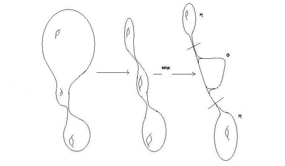
Figure 1: Large-scale picture of a cosmological solution. Observe that the reduced volume ${\mathcal{V}}$ is represented as decreasing.

A crucial quantity used in the proof of Theorem 1 is the reduced volume ${\mathcal{V}}={\mathcal{H}}^{3}V_{g({\mathcal{H}})}$ which is the volume of the cosmologically normalized metric $\tilde{g}$. As it turns out [3] the reduced volume (which is scale invariant) is either monotonically decreasing or steady in which case the solution is a flat cone. Equally important, the infimum of the reduced volume when it is thought as a function on CMC states $(g,K)$ (i.e. pairs $(g,K)$ satisfying the constraint equations) is given by ${\mathcal{V}}_{inf}=(\frac{-Y(\Sigma)}{-6})^{\frac{3}{2}}$ [3]. The natural question is whether it is always the case that ${\mathcal{V}}\downarrow{\mathcal{V}}_{inf}$ at least under the curvature assumption above. If it does so, it is known ([1] Theorem 9) that the geometrization is strong and (therefore) unique. We will call it the Thurston geometrization. We conjecture that such is always the case for solutions satisfying the curvature assumption.

Conjecture 1

Say $Y(\Sigma)\leq 0$ and say $(\tilde{g},\tilde{K})$ is a cosmologically normalized Einstein flow satisfying the assumption. Then ${\mathcal{V}}\downarrow{\mathcal{V}}_{inf}=(\frac{-Y(\Sigma)}{6})^{\frac{3}{2}}$.

Another way to express the conjecture is that the Thurston geometrization is a global attractor for cosmologically normalized flows satisfying the curvature assumption on manifolds with non-positive Yamabe invariant. If valid, the conjecture implies that the (scale invariant) Yamabe functional

$$Y(g)=\frac{\int_{\Sigma}R_{g}dv_{g}}{V_{g}^{\frac{1}{3}}},$$

converges to the Yamabe invariant $Y(\Sigma)$ along the flow. This can be sketchily seen as follows. Under the curvature assumption the scalar curvature $R_{\tilde{g}}$ is known to be bounded (above and below, see Prop 2 later). On the other hand it is known that for manifolds with $Y(\Sigma)\leq 0$ it is [5] $(\frac{-Y(\Sigma)}{6})^{\frac{3}{2}}=\sum_{i=1}^{i=n}Vol_{\tilde{g}_{H,i}}(H_{i})$ where $H_{i}$ are the hyperbolic pieces in the Thurston decomposition of $\Sigma$. If ${\mathcal{V}}\downarrow{\mathcal{V}}_{inf}$ the volume of the $G$ sector collapses to zero and therefore $\frac{\int_{G}R_{\tilde{g}}dv_{\tilde{g}}}{V_{\tilde{g}}^{\frac{1}{3}}}\rightarrow 0$. As $R_{\tilde{g}}\rightarrow-6$ on the $H$ sector we have $Y(\tilde{g})=Y(g)\rightarrow Y(\Sigma)$ as desired.

The second main result will be to show that always the $G$ sector collapses in (reduced) volume .

Theorem 2

Say $Y({\Sigma})\leq 0$ and say $(\tilde{g},\tilde{K})$ is a cosmologically normalized flow satisfying the curvature assumption. Then the reduced volume of the total space converges towards the volume value of the long time geometrization.

The volume value of the geometrization (see also the background section) is

$\sum_{i=1}^{i=n}V_{g_{H,i}}(H_{i})$. This result is a first step to prove the conjecture above. In fact it validates the conjecture in some particular cases described in the Corollaries 1-4 which will be proved after the proof of Theorem 2 .

Corollary 1

Say $Y(\Sigma)\leq 0$. Given $\Lambda$ there is $\epsilon$ such that for any cosmologically normalized flow satisfying the curvature assumption (with the same $\Lambda$) and having ${\mathcal{V}}-{\mathcal{V}}_{inf}\leq\epsilon$ at an initial time, it is ${\mathcal{V}}\downarrow{\mathcal{V}}_{inf}$ in the long time.

In basic terms, what Corollary 1 says is that if we restrict to the set of solutions satisfying the curvature assumption with a fixed $\Lambda$ then the Thurston geometrization is stable (in the class).

Corollary 2

Say $Y(\Sigma)\leq 0$ and say $(\tilde{g},\tilde{K})$ is a cosmologically normalized flow satisfying the curvature assumption that is locally collapsing at every point, i.e. there is no $H$ sector in the long time geometrization. Then $Y(\Sigma)=0$ and ${\mathcal{V}}\downarrow{\mathcal{V}}_{inf}=0$.

Let ${\mathcal{V}}_{0}$ be the infimum of the volumes of all complete hyperbolic manifolds (with sectional curvature normalized to one), with or without cusps (this number is known to be positive [10]). Then we have

Corollary 3

Say $Y(\Sigma)\leq 0$ and say $(\tilde{g},\tilde{K})$ is a cosmologically normalized flow satisfying the curvature assumption. If at an initial time it is ${\mathcal{V}}<{\mathcal{V}}_{0}$ then ${\mathcal{V}}\downarrow{\mathcal{V}}_{inf}=0$ in the long time.

Corollary 3 says that if we restrict to the class of solutions satisfying the curvature assumption (with variable $\Lambda$), there is a threshold ${\mathcal{V}}_{0}$ for ${\mathcal{V}}$ at the initial time, below which the long time gemetrization has only a $G$ sector and the reduced volume collapses to zero in the long time.

Corollary 4

Say $Y(\Sigma)\leq 0$ and say $(\tilde{g},\tilde{K})$ is a cosmologically normalized flow satisfying the curvature assumption above. Then ${\mathcal{V}}\downarrow{\mathcal{V}}_{inf}$ iff the tori separating the $H$ and $G$ sectors in the long time geometrization of the flow are incompressible in $\Sigma$.

Corollary 4 shows that to prove Conjecture 1 is sufficient to prove the topological fact that the two-tori separating the $H$ and $G$ sectors are incompressible.

Finally as an outcome of the proof of Theorems 1 and 2 we will be able to prove

Corollary 5

Say $Y(\Sigma)\leq 0$ and say $(\tilde{g},\tilde{K})$ is a cosmologically normalized flow satisfying the curvature assumption. Then the Bel-Robinson energy $Q_{0}({\bf Rm})$ is an $o({\mathcal{H}})$ (i.e. $\lim_{{\mathcal{H}}\rightarrow 0}Q_{0}/{\mathcal{H}}=0$).

2 Background and terminology

2.1 Convergence and collapse of Riemannian manifolds

We will make use the Cheeger-Gromov theory of convergence and collapse of Riemannian three-manifolds under curvature bounds. In particular we will use extensively the following result ([4] Prop 4 and 5. See also [13])

Proposition 1

Let $(\Sigma_{i},g_{i})$ be a sequence of Riemannian three-manifolds with or without boundary, with uniformly bounded $C^{\alpha}_{g_{i}}$ Ricci curvature, i.e. $\|Ric_{g_{i}}\|_{C^{\alpha}_{g_{i}}}\leq\Lambda$. We have

1. say $\{x_{i}\}$ is a sequence of points such that $dist(x_{i},\partial\Sigma_{i})\rightarrow\infty$ and $inj_{g_{i}}(x_{i})\geq inj_{0}$. Then one can extract a subsequence $(\Sigma_{i_{j}},x_{i_{j}},g_{i_{j}})$ converging in $C^{2,\beta}$ to $(\Sigma_{\infty},x_{\infty},g_{\infty})$ ($\beta<\alpha$),

2. suppose non of the $(\Sigma_{i}$ is diffeomorphic to a closed space form (a quotient of $S^{3}$). Then for any $\epsilon>0$ and $inj_{0}$ there is $r(\epsilon,\Lambda,inj_{0})$ with $r\rightarrow\infty$ as $\epsilon\rightarrow 0$, such that if $dist(x_{i},\partial\Sigma_{i})\geq r$ there is a finite cover of the ball $B(x_{i},r)$ with $inj_{g_{i}}(x_{i})\sim inj_{0}$.

A number of remarks are in order.

i) If $U$ is any tensor field on a Riemannian manifold $(\Sigma,g)$ then the $C^{k,\alpha}_{g}$ norm of $U$ is defined as

$$\begin{split}\|U\|_{C^{k,\alpha}_{g}}&=sup_{x\in\Sigma}\{|U|_{g}(x)+|\nabla U|_{g}(x)+\dots+|\nabla^{k}U|_{g}(x)+\\ &\quad sup_{y\in\Sigma}\{\frac{|\nabla^{k}U(x)-\nabla^{k}U(y)|}{dist(x,y)^{\alpha}}\}\}.\end{split}$$

The difference $\nabla^{k}U(x)-\nabla^{k}U(y)$ is by parallel transport along any shortest geodesic joining $x$ with $y$.

ii) The convergence in item 1 in the Proposition above is in the following sense: there is a sequence of submanifolds $\tilde{\Sigma}_{i}\subset\Sigma_{i}$ with $x_{i}\in\tilde{\Sigma_{i}}$ and $dist(x_{i},\partial\tilde{\Sigma_{i}})\rightarrow\infty$ and a sequence of diffeomorphisms (onto the image) $\varphi_{i}:\tilde{\Sigma}_{i}\rightarrow\Sigma_{i}$ such that $\|\varphi_{i*}(g_{i})-g_{\infty}\|_{C^{2,\beta}_{g_{\infty}}}\rightarrow 0$.

c) A sequence of tensors $U_{i}$ in $(\Sigma_{i},x_{i},g_{i})$ converge in $C^{k,\beta}$ to $U_{\infty}$ in $(\Sigma_{\infty},x_{\infty},g_{\infty})$ if $\|\varphi_{i*}U_{i}-U_{\infty}\|_{C^{k,\beta}_{g_{\infty}}}\rightarrow 0$.

d) One practical consequence of Proposition 1 is that when it comes to find interior elliptic estimates of certain elliptic operators on collapsed regions, we may well assume (because we can unwrap) that at the given point $x$ where one wants to extract the estimate there is a chart $(z_{1},z_{2},z_{3})$ of harmonic coordinates covering the ball $B(x,inj_{0})$ with $g_{ij}$ (the components of $g$ in the chart $\{z\}$) bounded in $C^{2,\alpha}_{\{z\}}$ (now the norms are standard Hölder norms on the chart $\{z\}$) by a constant $C(inj_{0},\Lambda)$. We will be using this fact repeatedly all through the article.

2.2 Electric-magnetic decomposition of the space-time curvature and some related formulae

In this section we introduce the electric/magnetic decomposition of the space-time curvature and useful formulae. Non of the properties presented is given with a proof. The reader can consult the references [7],[8] for a detailed account on Weyl fields.

Let $T$ be the normal unit vector field in the future direction and say ${\bf g}$ is a vacuum solution of the Einstein equations. Then the electric and magnetic fields of ${\bf Rm}$ are defined by

$$E_{ab}={\bf Rm}_{acbd}T^{c}T^{d},\ \ B_{ab}=^{*}{\bf Rm}_{acbd}T^{c}T^{d}.$$

The electric and magnetic fields are traceless and $T$-null $(2,0)$ vectors. In terms of $g$ and $K$ they have the expressions

$$E=Ric+kK-K\circ K,\ \ B=-CurlK,$$

where $Curl$ is the operator on symmetric $(2,0)$ tensors defined as $(CurlA)_{ab}=\frac{1}{2}(\epsilon_{a}^{\ cd}\nabla_{d}A_{cb}+\epsilon_{b}^{\ cd}\nabla_{d}A_{ca})$ ($\epsilon_{abc}$ is the volume form). We also have

$$DivE=K\wedge B,\ \ DivB=-K\wedge B,$$

where $(DivA)_{a}=\nabla^{b}A_{ba}$ is the divergence and $\wedge$ is the operation $(A\wedge C)_{a}=\epsilon_{a}^{\ bc}A_{b}^{\ d}C_{dc}$. Dynamically (under zero shift) we have

$$\dot{E}=NCurlB-\nabla N\wedge B-\frac{5}{2}N(E\times K)-\frac{2}{3}N<E,K>g-\frac{1}{2}NkE,$$

$$\dot{B}=-NCurlE+\nabla N\wedge E-\frac{5}{2}N(B\times K)-\frac{2}{3}N<B,K>k-\frac{1}{2}NkB.$$

the dot meaning derivative with respect to $k$, $<.,.>$ is the inner product and $\times$ is the operation

$$(A\times C)_{ab}=\epsilon_{a}^{\ cd}\epsilon_{b}^{\ ef}A_{ce}C_{df}+\frac{1}{3}(A.C)g_{ab}-\frac{1}{3}(trA)(trC)g_{ab}.$$

The Bel-Robinson tensor is the totally symmetric, traceless, $(4,0)$ tensor $Q_{\alpha\beta\gamma\delta}$, defined as

$$Q_{\alpha\beta\gamma\delta}={\bf Rm}_{\alpha\mu\gamma\nu}{\bf Rm}_{\beta\ \delta}^{\ \mu\ \nu}+{\bf Rm}_{\alpha\mu\gamma\nu}^{*}{\bf Rm}^{*\ \mu\ \nu}_{\beta\ \delta}.$$

We have $Q_{\alpha\beta\gamma\delta}({\bf Rm})T^{\alpha}T^{\beta}T^{\gamma}T^{\delta}=|E|^{2}_{g}+|B|^{2}_{g}$ and $\nabla^{\alpha}Q_{\alpha\beta\gamma\delta}({\bf Rm})=0$. Denote by $Q$ the integral in $\Sigma$ of $Q_{TTTT}$. Taking the divergence of $Q_{\alpha TTT}$ and integrating we get the Gauss equation

$$\dot{Q}=-3\int_{\Sigma}NQ_{\alpha\beta TT}{\bf\Pi}^{\alpha\beta}dv_{g}.$$

where ${\bf\Pi}$ is the deformation tensor ${\bf\Pi}_{\alpha\beta}=$$\nabla$${}_{\alpha}T_{\beta}$. Restricted to any CMC slice we have ${\bf\Pi}=-K$, ${\bf\Pi}_{Ti}=\frac{1}{N}\nabla_{i}N$, ${\bf\Pi}_{Ti}=0$ and ${\bf\Pi}_{TT}=0$. Again dot means derivative with respect to $k$. All through the article we will use the formulae above but for the cosmologically normalized tensors. We will indicate that by using a tilde above the referred tensor or by including a subindex $\tilde{g}$ next to tensor operation, for instance $\wedge_{\tilde{g}}$ or $|(.)|_{\tilde{g}}$. The cosmological normalized versions of the equations above is straightforward to get and won’t be deduced when needed.

2.3 The Newtonian potential, the reduced volume element and the logarithmic time

When working with cosmologically normalized quantities, it is convenient to use the logarithmic time $\sigma=-\ln-k$ as the time variable. Derivatives with respect to $\sigma$ of a cosmologically normalized quantity gives rise to a quantity which is also cosmologically normalized. For the rest of the article derivatives with respect to $\sigma$ will be denoted with a dot.

To illustrate how to work with cosmologically normalized quantities let us introduce the Newtonian potential $\phi=3\tilde{N}-1=3N{\mathcal{H}}^{2}-1$ and the reduced volume element $d\nu={\mathcal{H}}^{3}dv_{g}$ (both are scale invariant) and let us deduce the following pair of equations which will be fundamental

(7) $$\frac{\ln(d\nu)^{\frac{1}{3}}}{d\sigma}=\phi,$$

(8) $$\Delta_{\tilde{g}}\phi-|\tilde{K}|^{2}_{\tilde{g}}\phi=|\tilde{\hat{K}}|^{2}_{\tilde{g}}.$$

We have used a hat $\hat{}$ above $\tilde{K}$ to mean the traceless part of $\tilde{K}$ (with respect to $\tilde{g}$). Under zero shift we have

$$\frac{ddv_{g}}{dk}=\frac{1}{2}tr_{g}\frac{dg}{dk}dv_{g}=-Nkdv_{g}.$$

Now $d/d\sigma=(d/dk)(dk/d\sigma)=-kd/dk$ and so

(9) $$\frac{d\ln(d\nu)^{\frac{1}{3}}}{d\sigma}=\frac{d\ln{\mathcal{H}}}{d\sigma}+{\mathcal{H}}(N{\mathcal{H}}/3)=3N{\mathcal{H}}^{2}-1,$$

as desired. To get the Poisson-like equation for the Newtonian potential $\phi$ observe that the lapse equation (6) is scale invariant and therefore

$$-\Delta_{\tilde{g}}\tilde{N}+|\tilde{K}|^{2}_{\tilde{g}}\tilde{N}=1.$$

Making $\tilde{N}=\frac{1}{3}(\phi+1)$ we get

$$-\Delta_{\tilde{g}}\phi+|\tilde{K}|^{2}_{\tilde{g}}\phi=3-|\tilde{K}|^{2}_{\tilde{g}}=-|\tilde{\hat{K}}|^{2}_{\tilde{g}}.$$

A final remark. The Maximum principle applied to (8) gives $-1\leq\phi\leq 0$. This important fact implies by equation (7) that the local reduced volume element $d\nu$ is non increasing (under zero shift) and in particular that the reduced volume ${\mathcal{V}}$ is monotonically decreasing unless is steady in which case the solution is a flat cone.

2.4 Geometric states and persistent geometric states

In this section we introduce some definitions, that although not strictly needed, puts the main concepts used in a broad geometric context.

Definition 1

Given a compact three-manifold $\Sigma$ define the geometric spectrum to be the set of all its partitions (geometric states) of the form $\Sigma=\{H_{1}\ldots,H_{i},G_{1},$

$\ldots,G_{j}\}$ where the $H$ pieces are three manifolds possibly with boundary admitting a complete hyperbolic metric of finite volume, and the $G$ are graph three-manifolds possibly with boundary. If any, the boundaries in all pieces are two-tori and a torus in the boundary of a $H$ piece is always a torus in the boundary of a $G$ piece. Two geometric states are said to be equivalent if there is an isotopy in $\Sigma$ carrying the $H$ and the $G$ sectors of one into the $H$ and $G$ sectors of the other. A geometric state is said to be pure if there is only a $H$ or a $G$ piece.

Definition 2

Given a geometric state $\{H_{1},\ldots,H_{i},G_{1},\ldots,G_{j}\}$, its volume value $V$ is defined as the sum of the volumes of the complete hyperbolic metrics of finite volume of the $H$ pieces. The volumetric spectrum is defined as the set of all the volume values for all the states in the geometric spectrum.

In this terminology, Theorem 1 says in particular that if $\epsilon$ is chosen sufficiently small then after sufficiently long time the $\epsilon$-thick-thin decomposition is a (persistent) geometric state of the manifold. We will prove in Theorem 2 that ${\mathcal{V}}$ decreases to the volume value of the geometric state in which the flow is decaying.

We make precise now the notion of persistence of a geometrization introduced in section $1$. These notions will be used in the proofs of the main results. We say that a long time, cosmologically normalized flow $(\tilde{g},\tilde{K})$ implements a persistent geometrization iff either

1. $inj_{\tilde{g}(\sigma)}(\Sigma)\rightarrow 0$ as $\sigma$ goes to infinity (in which case there is only one persistent $G$ piece) or

2. $inj_{\tilde{g}{\sigma}}(\Sigma)\geq inj_{0}>0$ as $\sigma$ goes to infinity (in which case there is only one persistent $H$ piece) and there is a continuous function $\varphi:(-\ln-a,\infty)\times H\rightarrow\Sigma$, differentiable in the second factor, such that $\|\varphi^{*}\tilde{g}(\sigma)-\tilde{g}_{H}\|_{C^{2,\beta}_{\tilde{g}_{H}}}\rightarrow 0$ as $\sigma$ goes to infinity, or

3. the injectivity radius collapses in some regions and remains bounded below in some others (in which case there are a set of $G$ pieces $G_{1},\ldots,G_{j}$ and a set of $H$ pieces $H_{1},\ldots,H_{k}$) and for any $\epsilon>0$ and for any $H$ piece $(H_{i},\tilde{g}_{Hi})$ there is a continuous function $\varphi_{i}:(-\ln-a,\infty)\times H^{\epsilon}_{i}\rightarrow\Sigma$, differentiable in the second factor such that $\|\varphi_{i}^{*}\tilde{g}(\sigma)-\tilde{g}_{Hi}\|_{C^{2,\beta}_{\tilde{g}_{Hi}}}\rightarrow 0$ as $\sigma$ goes to infinity.

2.5 Some useful terminology

Any sequence $\{\sigma_{i}\}$ of logarithmic times ($\sigma_{i}=-\ln-k_{i}$) which is diverging i.e. $\lim_{i\rightarrow\infty}\sigma_{i}=\infty$ will be called a diverging sequence of logarithmic times and abbreviated DSLT. Given a DSLT, $\{\sigma_{i}\}$, we say that a sequence of sets $\Omega(\sigma_{i})$ has asymptotically total reduced volume (ATRV) if ${\mathcal{V}}(\Omega(\sigma_{i}))\rightarrow{\mathcal{V}}_{\infty}$ as $\sigma_{i}\rightarrow\infty$ where ${\mathcal{V}}_{\infty}$ is the limit of the reduced volume in the long time. Similarly we can define a set having asymptotically non-zero (ANZRV) or asymptotically zero reduced volume (AZRV). We say that a quantity $f$ controls a quantity $h$ if $|f|<M$ implies $|h|<C(M)$, and $f$ controls $h$ at zero if $M\rightarrow 0$ implies $C(M)\rightarrow 0$.

3 Proof of the main results and corollaries

This section is organized as follows. We prove first three propositions (Propositions 2,3,4) that would frame the proofs of Theorem 1 and 2 . We prove then Theorems 1 and 2 and next the Corollaries 1-5.

Let us give a heuristic behind the proofs of Theorems 1 and 2 . The key ingredient is to look at the reduced volume. As it is monotonic, it must settle in some limit value ${\mathcal{V}}_{\infty}$ as ${\mathcal{H}}\rightarrow 0$. Therefore in the regions where the injectivity radius is bounded below (in $(\Sigma,\tilde{g}(\sigma)))$ it must be $\phi\sim 0$ otherwise by equation (7) the volume would keep decreasing and eventually become below ${\mathcal{V}}_{\infty}$. Using equation (8) this implies $|\tilde{\hat{K}}|^{2}_{\tilde{g}}\sim 0$ which after using the Einstein equations implies $|\tilde{\hat{Ric}}|^{2}_{\tilde{g}}\sim 0$. In other words the regions where the injectivity radius remains bounded below become hyperbolic. This argument gives in essence Theorem 1 . Theorem 2 is more involved because it deals with the regions where the injectivity radius collapses. We are able to show however that if the $G$ regions (where the injectivity radius collapses) carry a non zero reduced volume (call it ${\mathcal{V}}_{0}$), then the regions inside $G$ whose unwrapped geometry becomes hyperbolic carry asymptotically all the volume ${\mathcal{V}}_{0}$. This fact will imply an isoperimetric inequality showing that the regions lying at a distance between 1/2 and 1 from the collapsed regions and whose unwrapped geometry is becoming hyperbolic, carry also asymptotically a non zero reduced volume (if ${\mathcal{V}}_{0}\neq 0$). As these two regions are disjoint, the limit of the volume of the $G$ regions must be above ${\mathcal{V}}_{0}$ which is a contradiction.

Proposition 2

Say $Y(\Sigma)\leq 0$ and say $(\tilde{g},\tilde{K})$ is a cosmologically normalized flow satisfying the curvature assumption. At any logarithmic time $\sigma$ we have the following properties.

1. $\|\tilde{\hat{K}}\|_{C^{1,\alpha}_{\tilde{g}}}$, $\|\tilde{\hat{Ric}}\|_{C^{\alpha}_{\tilde{g}}}$ and $\|\phi\|_{C^{2,\alpha}_{\tilde{g}}}$ are controlled by $\Lambda$.

2. For any $\epsilon>0$ there is $\delta(\epsilon,\Lambda)>0$ such that at any point $p$ if $|\phi(p)|\leq\delta$ then $|\tilde{\hat{K}}|_{\tilde{g}}(p)\leq\epsilon$. In other words $-\phi(p)$ controls $|\tilde{\hat{K}}|_{\tilde{g}}(p)$ at zero.

Proof:

1. As has been proved in [4] (Prop 2.2), $\|\tilde{K}\|_{L^{\infty}_{\tilde{g}}}$ and $\|Ric\|_{L^{\infty}_{\tilde{g}}}$ are controlled by $\Lambda$. Consider the elliptic system

$$Div\tilde{\hat{K}}=0,$$

$$Curl_{\tilde{g}}\tilde{\hat{K}}=-B,$$

Pick a point $x\in\Sigma$ and unwrap if necessary to have $inj_{\tilde{g}}(x)\geq inj_{0}$. Then interior Schauder estimates [14] show that $\|\tilde{\hat{K}}\|_{C^{1,\alpha}_{\tilde{g}}(B(x,inj_{0}/2))}$ is controlled by $\Lambda$. Therefore $\|\tilde{\hat{K}}\|_{C^{1,\alpha}_{\tilde{g}}}$ is controlled by $\Lambda$. From $E=\tilde{Ric}-3\tilde{K}+\tilde{K}\circ\tilde{K}$ we get that $\|\tilde{Ric}\|_{C^{\alpha}_{\tilde{g}}}$ is controlled by $\Lambda$. Schauder estimates applied to

$$\Delta_{\tilde{g}}\phi-|\tilde{\hat{K}}|^{2}_{\tilde{g}}\phi=|\tilde{K}|^{2}_{\tilde{g}},$$

show that $\|\phi\|_{C^{2,\alpha}_{\tilde{g}}}$ is controlled by $\Lambda$.

2. Suppose there is a sequence of logarithmic times $\{\sigma_{i}\}$ and a sequence of points $\{x_{i}\}$ such that $\phi(x_{i},\sigma_{i})\rightarrow 0$ but $|\tilde{\hat{K}}|_{\tilde{g}(\sigma_{i})}(x_{i},\sigma_{i})\geq M$ with $M>0$. Unwrapping if necessary to have $inj_{\tilde{g}}(x_{i})\geq inj_{0}$ we can extract a subsequence of $\{\sigma_{i}\}$ such that on the balls $B(x_{i},inj_{0}/2)$, $\tilde{g}(\sigma_{i})$ converges in $C^{2,\beta}$ to a limit metric $\tilde{g}_{\infty}$, $\phi$ converges in $C^{2,\beta}$ to a limit $\phi_{\infty}\leq 0$ with $\phi_{\infty}(x_{\infty})=0$ and $\tilde{\hat{K}}$ converges in $C^{1,\beta}$ to a limit $\tilde{\hat{K}}_{\infty}$ with $|\tilde{\hat{K}}|_{\tilde{g}_{\infty}}(x_{\infty})\geq M$, all satisfying the equation

$$\Delta_{\tilde{g}_{\infty}}\phi_{\infty}-|\tilde{K}_{\infty}|^{2}_{\tilde{g}_{\infty}}\phi_{\infty}=|\tilde{\hat{K}}|^{2}_{\tilde{g}_{\infty}}.$$

However at $x_{\infty}$ it is $0\geq(\Delta_{\tilde{g}_{\infty}}\phi_{\infty})(x_{\infty})=|\tilde{\hat{K}}|^{2}_{\tilde{g}_{\infty}}(x_{\infty})>M>0$ which is absurd. $\Box$

Proposition 3

Say $\Sigma$ is a compact three-manifold with bounded $C^{\alpha}_{g}$ norm of the curvature and bounded volume, i.e. $\|Ric\|_{C^{\alpha}_{g}}+Vol_{g}(\Sigma)\leq\Lambda$, and say $r<r^{\prime}$. Then there is $C(\Lambda,r,r^{\prime})$ such that for any measurable subset $\Omega$ it is $Vol_{g}(B(\Omega,r))\geq C(\Lambda,r,r^{\prime})Vol_{g}(B(\Omega,r^{\prime}))$ where $B(\Omega,s)$ is the ball of $\Omega$ with radius $s$.

Proof:

Let ${\mathcal{K}}(\Lambda)<0$ be a lower bound for the sectional curvatures of any Riemannian three-manifold with $\|Ric\|_{L^{\infty}_{g}}\leq C(\Lambda)$. Let $\{x_{i},i=1,\ldots,m\}\subset\Sigma$ be any set of $m$ points. By the Bishop-Gromov volume comparison the function

$Vol_{g}(\cup_{i=1}^{i=m}B(x_{i},r))/Vol_{g_{{\mathcal{K}}}}(o,r)$ is monotonically decreasing as $r$ increases, where $g_{\mathcal{K}}$ is a metric of constant sectional curvature ${\mathcal{K}}$ in $\mathbb{R}^{3}$. We have therefore

(10) $$Vol_{g}(\cup_{i=1}^{i=m}B(x_{i},r^{\prime}))\leq C(\Lambda,r,r^{\prime})Vol_{g}(\cup_{i=1}^{i=m}B(x_{i},r)),$$

for any $r<\bar{r}$. Now consider a measurable set $\Omega$. There is $\{x_{i},i=1,\ldots,\infty\}\subset\Omega$ such that

$$\cup_{i=1}^{i=m}B(x_{i},r)\uparrow_{m}B(\Omega,r),$$

and

$$\cup_{i=1}^{i=m}B(x_{i},r^{\prime})\uparrow B(\Omega,r^{\prime}).$$

Then taking volumes we have

$$\begin{split}Vol_{g}(B(\Omega,r^{\prime}))&=\lim_{m\rightarrow\infty}Vol_{g}(\cup_{i=1}^{i=m}B(x_{i},r^{\prime}))\leq C(\Lambda,r,r^{\prime})\lim_{m\rightarrow\infty}Vol_{g}(\cup_{i=1}^{i=m}B(x_{i},r))\\ &=C(\Lambda,r,r^{\prime})Vol_{g}(B(\Omega,r)),\end{split}$$

which finishes the proof. $\Box$

Proposition 4

Say $Y(\Sigma)\leq 0$ and say $(\tilde{g},\tilde{K})$ is a cosmologically normalized flow satisfying the curvature assumption. We have the following properties.

1. Given $\Gamma\geq 0$ and any DSLT, $\{\sigma_{i}\}$, the sequence of sets $\Omega_{\phi,\Gamma}(\sigma_{i})=\{x\in\Sigma/-\phi(x,\sigma_{i})\geq\Gamma\}$ has AZRV.

2. Given $\Gamma\geq 0$ and any DSLT, $\{\sigma_{i}\}$, the sequence of sets $\Omega_{\tilde{\hat{K}},\Gamma}(\sigma_{i})=\{x\in\Sigma/|\tilde{\hat{K}}(x,\sigma_{i})|_{\tilde{g}(\sigma_{i})}\geq\Gamma\}$ has AZRV.

3. Given $\Gamma\geq 0$ and any DSLT, $\{\sigma_{i}\}$, the sequence of sets $\Omega_{\nabla\tilde{\hat{K}},\Gamma}=\{x\in\Sigma/|\nabla\tilde{\hat{K}}(x,\sigma_{i})|_{\tilde{g}(\sigma_{i})}\geq\Gamma\}$ has AZRV.

4. For any pair of DSLT, $\{\sigma_{i}\}$ and $\{\sigma^{\prime}_{i}\}$ with $\delta^{\prime}\geq\sigma_{i}-\sigma^{\prime}_{i}\geq\delta$ ($\delta^{\prime}>\delta>0$ and fixed) we have

   $$\int_{\sigma^{\prime}_{i}}^{\sigma_{i}}\|E\|^{2}_{L^{2}_{\tilde{g}(\sigma)}}d\sigma\rightarrow 0.$$

5. For any DSLT $\{\sigma_{i}\}$ we have

   $$\tilde{Q}_{0}(\sigma_{i})=(\|E\|^{2}_{L^{2}_{\tilde{g}}}+\|B\|^{2}_{L^{2}_{\tilde{g}}})(\sigma_{i})\rightarrow 0.$$

   and therefore the sets

   $$\Omega_{B,\Gamma}(\sigma_{i})=\{x\in\Sigma/|B(x,\sigma_{i})|_{\tilde{g}(\sigma_{i})}\geq\Gamma\},$$

   $$\Omega_{\tilde{\hat{Ric}},\Gamma}(\sigma_{i})=\{x\in\Sigma/|\tilde{\hat{Ric}}(x_{i},\sigma_{i})|_{\tilde{g}(\sigma_{i})}\geq\Gamma\},$$

   have AZRV.

Proof:

1. Differentiating

$$\Delta_{\tilde{g}}\phi-|\tilde{K}|^{2}_{\tilde{g}}\phi=|\tilde{\hat{K}}|^{2}_{\tilde{g}},$$

with respect to logarithmic time we get

(11) $$\Delta_{\tilde{g}}\dot{\phi}-|\tilde{K}|^{2}_{\tilde{g}}\dot{\phi}=-({\Delta}_{\tilde{g}})\dot{}\phi+(|\tilde{K}|^{2}_{\tilde{g}})\dot{}\phi+(|\tilde{\hat{K}}|^{2}_{\tilde{g}})\dot{}.$$

Appealing to

$$\dot{\tilde{g}}=2\phi\tilde{g}-6\tilde{N}\tilde{\hat{K}},$$

$$\dot{\tilde{\hat{K}}}=-\tilde{\hat{K}}-\phi\tilde{g}-\nabla^{2}\phi+\phi E+E-\tilde{N}(\tilde{\hat{K}}\circ\tilde{\hat{K}}-2\tilde{\hat{K}}),$$

$$(\Delta_{\tilde{g}})\dot{}(\phi)=<\nabla^{2}\phi,\dot{\tilde{g}}>_{\tilde{g}}-<\nabla\phi,Div\dot{\tilde{g}}+\frac{1}{2}dtr_{\tilde{g}}\dot{\tilde{g}}>_{\tilde{g}},$$

we get by Proposition 2 1 that the right hand side of equation (11) has $C^{\alpha}$ norm controlled by $\Lambda$. By the maximum principle on equation (11) $\|\dot{\phi}\|_{L^{\infty}}$ is controlled by $\Lambda$. Therefore writing $\phi(x,\sigma)-\phi(x,\sigma_{i})=\int_{\sigma_{i}}^{\sigma}\dot{\phi}(x,\sigma)d\sigma$ we see that if $-\phi(x,\sigma_{i})\geq\Gamma$ there is $T(\Lambda,\Gamma)$ such that $-\phi(x,\sigma)\geq\Gamma/2$ for every $\sigma\in[\sigma_{i},\sigma_{i}+T(\Lambda,\Gamma)]$. Now suppose there is a subsequence of $\{\sigma_{i}\}$ denoted by $\{\sigma_{i_{j}}\}$ such that ${\mathcal{V}}(\Omega_{\phi,\Gamma}(\sigma_{i_{j}}))\geq M$ for some $M>0$, then $\dot{\mathcal{V}}(\sigma)=\int_{\Sigma}(d\nu)\dot{}=\int_{\Sigma}3\phi d\nu\leq-3MT(\Lambda)/2$ for any $\sigma\in[\sigma_{i_{j}},\sigma_{i_{j}}+T(\Lambda,\Gamma)]$. Therefore as ${\mathcal{V}}$ is monotonic, it must be ${\mathcal{V}}(\sigma)\downarrow-\infty$ as $\sigma\rightarrow\infty$ which is absurd.

2. This is direct from 1 above and Proposition 2 2.

3. We prove first the claim that if $|\nabla\tilde{\hat{K}}(x,\sigma)|_{\tilde{g}}\geq\Gamma$ then there is $r(\Lambda,\Gamma)$ and $x^{\prime}\in B(x,r)$ such that $|\tilde{\hat{K}}(x^{\prime},\sigma)|_{\tilde{g}}\geq M$ for some $M(\Lambda,\Gamma)>0$. This shows that $\Omega_{\nabla\tilde{\hat{K}},\Gamma}(\sigma)\subset B(\Omega_{\tilde{\hat{K}},M}(\sigma),r)$. Once this is proved, by Propositions 3 and 4 2 $B(\Omega_{\tilde{\hat{K}},M}(\sigma_{i}),r)$ and therefore $\Omega_{\nabla\tilde{\hat{K}},\Gamma}(\sigma_{i})$ have AZRV which would finish this item. Now let us prove the claim. From now on if at $x$, $inj_{\tilde{g}(\sigma)}(x)$ is small we unwrap to have $inj_{\tilde{g}(\sigma)}(x)\geq inj_{0}>0$. By Proposition 2 1 we have that $\nabla\tilde{\hat{K}}$ is controlled in $C^{\alpha}$, therefore $|\nabla\tilde{\hat{K}}(x,\sigma)-\nabla\tilde{\hat{K}}(y,\sigma)|_{\tilde{g}}\leq C(\Lambda)d(x,y)^{\alpha}$. Pick a unit vector $v(x)$ at $x$ such that $|\nabla_{v}\tilde{\hat{K}}(x,\sigma)|_{\tilde{g}}\geq\Gamma/3$. Pick a harmonic chart $\{x^{i}\}$ covering the ball $B(x,inj_{0})$ such that the Christoffel symbols $\Gamma_{ij}^{k}$ are zero at $x$ (this is always possible) and write in the $\{x^{i}\}$ coordinates

$$(\nabla_{v}\tilde{\hat{K}})_{jk}(y)=v^{i}\partial_{x^{i}}\tilde{\hat{K}}_{jk}(y)-\Gamma_{jk^{\prime}}^{l}(y)\tilde{\hat{K}}_{lk}(y)v^{k^{\prime}}(y)-\Gamma_{kk^{\prime}}^{l}(y)\tilde{\hat{K}}_{jl}(y)v^{k^{\prime}}(y).$$

Pick $r(\Lambda,\Gamma)\leq inj_{0}$ with $r^{\alpha}C(\Lambda)\leq\Gamma/20$ such that $|\Gamma_{ij}^{l}\tilde{\hat{K}}_{lk}|\leq\Gamma/40$ on $B(x,r)$. Then on $B(x,r)$ we have $|\partial_{v}\tilde{\hat{K}}(x)-\partial_{v}\tilde{\hat{K}}(y)|\leq\Gamma/10$ and therefore $|\tilde{\hat{K}}(p)-\tilde{\hat{K}}(q)|\geq\Gamma 2r/4$ where $p$ and $q$ are the intercepts of the line (in the coordinate system $\{x^{i}\}$) $x+\lambda v$ and the boundary of the ball $B(x,r)$. So either $|\tilde{\hat{K}}(p)|$ or $|\tilde{\hat{K}}(q)|$ must be greater or equal to $\Gamma r/4$. This finishes the proof of the claim.

4. We start by noting the following. Say $f$ and $h$ are tensorial quantities such that, given $\Gamma>0$ and any DSLT , $\{\sigma_{i}\}$, $\|h\|_{L^{\infty}_{\tilde{g}}}(\sigma_{i})$ and $\|f\|_{L^{\infty}_{\tilde{g}}}$ are controlled by $\Lambda$ and the sequence of sets $\Omega_{f,\Gamma}(\sigma_{i})=\{x\in\Sigma/|f(x,\sigma_{i})|_{\tilde{g}}\geq\Gamma\}$ has AZRV, then: a) for any DSLT, $\{\sigma_{i}\}$, it is $(\int_{\Sigma}|h*f|_{\tilde{g}}^{2}dv_{\tilde{g}})(\sigma_{i})\rightarrow 0$ ($*$ is some tensorial composition) and b) for any pair of DSLT, $\{\sigma_{i}\}$ and $\{\sigma^{\prime}_{i}\}$ as in the statement of this item (Prop 4, 4), it is $\int_{\sigma^{\prime}_{i}}^{\sigma_{i}}(\int_{\Sigma}|h*f|^{2}dv_{\tilde{g}})d\sigma\rightarrow 0$ as $\sigma_{i}\rightarrow\infty$. The claim a) is obvious by writing $|h*f|_{\tilde{g}}\leq c|h|_{\tilde{g}}|f|_{\tilde{g}}$ for some numeric $c$. For the claim b) observe that if the claim holds for $h=1$ it holds for any $h$. Now if it is false for $h=1$ we can extract a sequence of logarithmic times $\{\bar{\sigma}_{i}\}$ with $\sigma_{i}\geq\bar{\sigma}_{i}\geq\sigma^{\prime}_{i}$ and $(\int_{\Sigma}|f|_{\tilde{g}}^{2}dv_{\tilde{g}})(\bar{\sigma_{i}})\nrightarrow 0$ which contradicts a).

Now note that by 2 above, the claim a) and

$$Curl_{\tilde{g}}\tilde{K}=-B,$$

we have that for any DSLT $\{\bar{\sigma}_{i}\}$, $\|B\|_{L^{2}_{\tilde{g}}}(\sigma_{i})\rightarrow 0$.

We will prove this item by studying the quantity

(12) $$\int_{\Sigma}<E,\tilde{\hat{K}}>_{\tilde{g}}dv_{\tilde{g}},$$

and its derivative with respect to logarithmic time. Differentiating it with respect to $\sigma$ we get

(13) $$\begin{split}(\int_{\Sigma}<E,\tilde{\hat{K}}>_{\tilde{g}}dv_{\tilde{g}})\dot{}&=\int_{\sigma}<\dot{E},\tilde{\hat{K}}>_{\tilde{g}}+<E,\dot{\tilde{\hat{K}}}>_{\tilde{g}}-<E\circ\tilde{\hat{K}}_{\tilde{g}},\dot{\tilde{g}}>+\\ &\quad+3<E,\tilde{\hat{K}}>_{\tilde{g}}\phi dv_{\tilde{g}}.\end{split}$$

To estimate the terms on the right hand side of the last equation we appeal to the equations

(14) $$\dot{\tilde{g}}=2\phi\tilde{g}-6\tilde{N}\tilde{\hat{K}},$$

(15) $$\dot{E}=\tilde{N}Curl_{\tilde{g}}B-\frac{\nabla\tilde{N}}{\tilde{N}}\wedge_{\tilde{g}}B-\frac{5}{2}E\times_{\tilde{g}}\tilde{K}-\frac{2}{3}<E,\tilde{K}>_{\tilde{g}}\tilde{g}-\frac{3}{2}E,$$

(16) $$\dot{\tilde{\hat{K}}}=-\tilde{\hat{K}}-\phi\tilde{g}-\nabla^{2}\phi+\phi E+E-\tilde{N}(\tilde{\hat{K}}\circ\tilde{\hat{K}}-2\tilde{\hat{K}}).$$

Recall $3\tilde{N}=\phi+1$. Integrate both sides of equation 13 in the interval $[\sigma^{\prime}_{i},\sigma_{i}]$ and plug in the equations (15), (16), (14). By the claim a) above the left hand side (of the integrated equation) converges to zero as $i\rightarrow\infty$. Using the items 1, 2 and the claim b) above we get that the only terms on the right hand side (of the integrated equation) that may not converge to zero as $i\rightarrow\infty$ are

(17) $$\int_{\sigma^{\prime}_{i}}^{\sigma_{i}}\int_{\Sigma}<E,\nabla^{2}\phi>_{\tilde{g}}dv_{\tilde{g}}d\sigma,$$

(18) $$\int_{\sigma^{\prime}_{i}}^{\sigma_{i}}\int_{\Sigma}\tilde{N}<Curl_{\tilde{g}}B,\tilde{\hat{K}}>_{g}dv_{\tilde{g}}d\sigma,$$

and

(19) $$\int_{\sigma^{\prime}_{i}}^{\sigma_{i}}\int_{\Sigma}|E|^{2}_{\tilde{g}}dv_{\tilde{g}}d\sigma.$$

To show that the equation (17) and (18) converge to zero as $i\rightarrow\infty$ we integrate by parts. In equation (17) integration by parts gives

$$\int_{\sigma^{\prime}_{i}}^{\sigma_{i}}\int_{\Sigma}-<DivE,\nabla\phi>_{g}dv_{\tilde{g}}d\sigma,$$

which by the formula $Div_{\tilde{g}}E=\tilde{K}\wedge_{\tilde{g}}B$ and the claim b) above is guaranteed to converge to zero as $i\rightarrow\infty$. To integrate by parts on equation 18 invoke the formula

$$Div(U\wedge U^{\prime})=-<CurlU,U^{\prime}>+<U,CurlU^{\prime}>,$$

holding for any $U$ and $U^{\prime}$ traceless symmetric tensors. This gives

(20) $$\int_{\sigma^{\prime}_{i}}^{\sigma_{i}}\int_{\Sigma}<B,\nabla\tilde{N}*\tilde{\hat{K}}+\tilde{N}Curl\tilde{\hat{K}}>dv_{\tilde{g}}d\sigma,$$

($*$ is some tensor operation). After using the formula $Curl_{\tilde{g}}\tilde{\hat{K}}=-B$ in equation (20), claim b) above shows that all the expression goes to zero as $i\rightarrow\infty$. We are thus lead to conclude that the expression (19) goes to zero as $i\rightarrow\infty$ as desired.

5. We have shown in ${\it 4}$ that $\|B\|^{2}_{L^{2}_{\tilde{g}(\sigma_{i})}}$ goes to zero as $i\rightarrow\infty$ for any DSLT $\{\sigma_{i}\}$. To show that the same happens for $E$ we make use of the Bel-Robinson energy. Observe that $\frac{1}{\mathcal{H}}\int_{\Sigma}(|E|_{g}^{2}+|B|^{2}_{g})dv_{g}=\frac{1}{\mathcal{H}}\int_{\Sigma}Q_{TTTT}({\bf Rm})dv_{g}=\int_{\Sigma}Q_{\tilde{T}\tilde{T}\tilde{T}\tilde{T}}(\tilde{\bf Rm})dv_{\tilde{g}}=\int_{\Sigma}(|E|^{2}_{\tilde{g}}+|B|^{2}_{\tilde{g}})dv_{\tilde{g}}$. Using the Gauss equation we get

(21) $$\dot{\tilde{Q}}=\tilde{Q}-9\int_{\Sigma}\tilde{N}\tilde{Q}_{\alpha\beta\tilde{T}\tilde{T}}\tilde{\bf\Pi}^{\alpha\beta}dv_{\tilde{g}}.$$

Now suppose there is a DSLT, $\{\sigma_{i}\}$, such that $\int_{\Sigma}|E|^{2}_{\tilde{g}}dv_{g}>M$ for some $M>0$. As the right hand side of equation (21) is controlled by $\Lambda$ we can find $T(\Lambda,M)$ such that the integral in $\sigma$ of the right hand side of equation (21) on the interval $[\sigma_{i},\sigma_{i}+T]$ is, in absolute value, less than $M/2$ and therefore integrating equation (21) on the interval $[\sigma_{i},\sigma]$ with $\sigma\in[\sigma_{i},\sigma_{i}+T]$ we get $\tilde{Q}(\sigma)\geq M/2$. Therefore $\int_{\sigma_{i}}^{\sigma_{i}+T}\tilde{Q}d\sigma\geq TM/2$. However by ${\it 4}$ we know $\int_{\sigma_{i}}^{\sigma_{i}+T}\int_{\Sigma}|E|^{2}_{\tilde{g}}+|B|^{2}_{\tilde{g}}dv_{\tilde{g}}d\sigma\rightarrow 0$ which is a contradiction.

$\Box$

We are now ready to prove Theorems $1$ and $2$ (stated conveniently).

Theorem 3

Say $Y(\Sigma)\leq 0$ and say $(\tilde{g},\tilde{K})$ a cosmologically normalized flow satisfying the curvature assumption. Then $(\tilde{g},\tilde{K})$ induces a unique persistent geometrization on $\Sigma$.

Proof:

We prove first there is a DSLT, $\{\sigma_{i}\}$ with $(\Sigma^{\frac{1}{i}},(\tilde{g},\tilde{K})(\sigma_{i}))$ converging to

$\cup_{i=1}^{i=n}(H_{i},(\tilde{g}_{H,i},-\tilde{g}_{H,i}))$ (in $C^{2,\beta}$). Introduce a new variable $j=1,2,3,\ldots$. For $j=1$ find a sequence $\{\sigma_{1,i}\}$ with $(\Sigma^{1},\tilde{g}(\sigma_{1,i}))$ convergent in $C^{2,\beta}$. For $j=2$ find a subsequence $\{\sigma_{2,i}\}$ of $\{\sigma_{1,i}\}$ with $(\Sigma^{1/2},\tilde{g}(\sigma_{2,i}))$ convergent in $C^{2,\beta}$. Proceed similarly for all $j$ to have a double sequence $\{\sigma_{j,i}\}$. Now, the diagonal sequence $\{\sigma_{i,i}\}$, $(\Sigma^{1/i},\tilde{g}(\sigma_{i,i}))$ converges into a union of complete manifolds of finite volume, denoted as $\cup_{\nu}(M_{\nu},\tilde{g}_{\infty,\nu})$. By Proposition 4 2, $\tilde{K}(\sigma_{i,i})$ converges to $-\tilde{g}_{\infty,\nu}$ in $C^{1,\beta}$. By proposition 4 5 and the formula $E=\tilde{Ric}-3\tilde{K}+\tilde{K}\circ\tilde{K}$ we get that each metric $\tilde{g}_{\infty,\nu}$ is hyperbolic. Therefore, as there is a lower bound for the volume of complete hyperbolic manifolds of finite volume and the total volume of the limit space is bounded above, there must be a finite number of components, and we can write $\cup_{\nu}(M_{\nu},\tilde{g}_{\infty,\nu})=\cup_{i=1}^{i=n}(H_{i},\tilde{g}_{H,i})$.

We prove next that each component $(H_{j},\tilde{g}_{H,j})$ is persistent. For simplicity assume there is only one component and therefore $(\Sigma^{1/i},\tilde{g}(\sigma_{i,i}))$ converges in $C^{2,\beta}$ to $(H,\tilde{g}_{H})$. There are two possibilities according to whether the component is compact ot not, we discuss them separately.

1.(The compact case) Assume $(H,\tilde{g}_{H})$ is compact. Consider the space of metrics ${\mathcal{M}}_{H}$ in $H$. For every metric $g$ consider the orbit of $g$ under the diffeomorphism group. Denote such orbit by $o(g)$. Around $\tilde{g}_{H}$ consider a small (smooth) section ${\mathcal{S}}$ of ${\mathcal{M}}_{H}$ of $C^{2,\beta}_{\tilde{g}_{H}}$ metrics transverse to the orbits generated by the action on ${\mathcal{M}}_{H}$ of the diffeomorphism group . For an illustration see Figure 2.

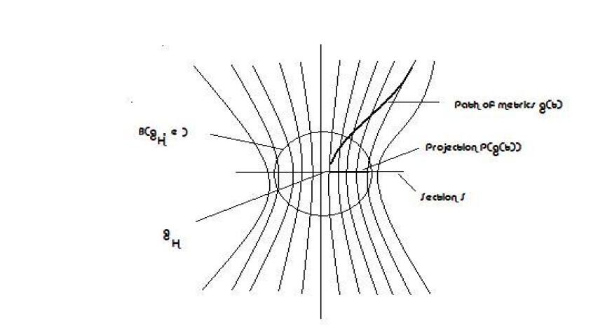
Figure 2: Representation of the space of metrics on a neighborhood of $\tilde{g}_{H}$.

If $\epsilon_{0}$ is sufficiently small every ($C^{\infty}$) metric $g$ in ${\mathcal{M}}_{H}$ with $\|g-\tilde{g}_{H}\|_{C^{2,\beta}_{\tilde{g}_{H}}}\leq\epsilon_{0}$ can be uniquely projected into ${\mathcal{S}}$ by a diffeomorphism, or in other words we can consider the projection $P(g)=o(g)\cap{\mathcal{S}}$. Note that one can project every $(C^{\infty}$) path of ($C^{\infty}$) metrics $g(t)$ starting close to $\tilde{g}_{H}$, to a $(C^{\infty})$ path $P(g(t))$, until at least the first time when $\|P(g(t))-\tilde{g}_{H}\|_{C^{2,\beta}_{\tilde{g}_{H}}}=\epsilon_{0}$ or in other words until at least when the projection touches the boundary of the ball of center $\tilde{g}_{H}$ and radius $\epsilon_{0}$ in $C^{2,\beta}_{\tilde{g}_{H}}$ (denote such ball as $B(\tilde{g}_{H},\epsilon_{0})$)

Recall Mostow rigidity Mostow rigidity (the compact case). There is $\epsilon_{1}$ such that if $P(g^{\prime}_{H})\in B(\tilde{g}_{H},\epsilon_{1})$, where $g^{\prime}_{H}$ is a hyperbolic metric in $H$ then $P(g^{\prime}_{H})=\tilde{g}_{H}$.

Fix $\epsilon_{2}=min\{\epsilon_{0},\epsilon_{1}\}$. Observe that as $\tilde{g}_{\sigma_{i,i}}\rightarrow\tilde{g}_{H}$ in $C^{2,\beta}$ there is a sequence of diffeomorphisms $\phi_{i}$ such that $\phi^{*}_{i}(g(\sigma_{i,i}))$ converges to $\tilde{g}_{H}$ in $C^{2,\beta}_{\tilde{g}_{H}}$. Now, if the geometrization is not persistent there is $\epsilon\leq\epsilon_{2}$ and $i_{2}$ such that if $i\geq i_{2}$ then $P(\phi^{*}_{i}(\tilde{g}(\sigma)))$ is well defined for $\sigma\geq\sigma_{i,i}$ until a first time $\sigma_{i,i}+T_{i}$ when $P(\phi^{*}_{i}(\tilde{g}(\sigma_{i,i}+T_{i})))$ is in $\partial B(\tilde{g}_{H},\epsilon_{2})$. But we know the sequence of Riemannian manifolds $(H,P(\phi^{*}_{i}(\tilde{g}(\sigma_{i,i}+T_{i}))))$ converge in $C^{2,\beta}$ to $\tilde{g}_{H}$, and that means by the definition of $C^{2,\beta}$ convergence and Mostow rigidity that there is a sequence of diffeomorphisms $\varphi_{i}$ such that $P(\varphi^{*}_{i}(P(\phi^{*}_{i}(\tilde{g}(\sigma_{i,i}+T_{i}))))$ converge to $\tilde{g}_{H}$ in $C^{2,\beta}_{\tilde{g}_{H}}$. This contradict the fact that $P(\phi^{*}_{i}(\tilde{g}(\sigma_{i,i}+T_{i})))$ is in $\partial B(\tilde{g}_{H},\epsilon_{2})$.

2. (The non-compact case). The proof of this case proceeds along the same lines as the compact case but special care must be taken at the cusps. Let us assume for simplicity that there is only one cusp in the piece $(H,\tilde{g}_{H})$. Given $A$ sufficiently small there is a unique torus transverse to the cusp, to be denoted by $T^{2}_{A}$, of constant mean curvature and area $A$. Denote by $H_{A}$ the “bulk” side of the torus $T^{2}_{A}$ in $H$. Consider the set of metrics ${\mathcal{M}}_{H_{A}}$ on $H_{A}$ such that for any of them $T^{2}_{A}$ has constant mean curvature and area $A$. Consider the action of the diffeomorphism group on ${\mathcal{M}}_{H_{A}}$ leaving the torus $T^{2}_{A}$ invariant. Again the orbit of $g$ will be denoted by $o(g)$. Consider a small (smooth) section of ${\mathcal{S}}$ of $C^{2,\beta}$ metrics around $\tilde{g}_{H}$ and transverse to the orbits of the action by the diffeomorphism group mentioned above. Finally consider the projection $P(g)=o(g)\cap{\mathcal{S}}$ which is well defined on a ball $B(\tilde{g}_{H},\epsilon_{0})$ for $\epsilon_{0}$ small enough. Observe again that a path $g(t)$ of metrics in ${\mathcal{M}}_{H_{A}}$ can be projected into ${\mathcal{S}}$ until at least the first time when $P(g(t))$ is in $\partial B(\tilde{g}_{H},\epsilon_{0})$. Slightly abusing the notation (as we would need a pointed sequence) consider the sequence $(\Sigma,\tilde{g}(\sigma_{i,i}))$ converging in $C^{2,\beta}$ to $\tilde{g}_{H}$. If $i\geq i_{0}$ we can identify on $\Sigma$ a torus $T^{2}_{A,\tilde{g}(\sigma_{i,i})}$ of constant mean curvature and area $A$ which converges as $i\rightarrow\infty$ (and after the application of a diffeomorphism) to $T^{2}_{A}$ in $H$. More in particular there is a sequence of diffeomorphisms (onto the image) $\phi_{i}:H_{A}\rightarrow\Sigma$ such that $\phi_{i}(T^{2}_{A})=T^{2}_{A,\tilde{g}(\sigma_{i,i})}$ and $\|\phi^{*}_{i}(\tilde{g}(\sigma_{i,i}))-\tilde{g}_{H}\|_{C^{2,\beta}_{\tilde{g}_{H}}}$ converging to zero. We note the following crucial facts (justified below).

i) The diffeomorphisms (onto the image) $\phi_{\sigma}:H_{A}\rightarrow\Sigma$ with $\phi_{\sigma}(T^{2}_{A})=T^{2}_{A,\tilde{g}(\sigma)}$ can be defined (varying differentiably) as long as the tori $T^{2}_{A,\tilde{g}(\sigma)}$ are well defined (varying differentiably).

ii) There are $\sigma_{0}$ and $\epsilon_{1}$ such that if $\sigma_{1}\geq\sigma_{0}$ and $\phi_{\sigma_{1}}:H_{A}\rightarrow\Sigma$ is well defined and $\|\phi^{*}_{\sigma_{1}}(\tilde{g}(\sigma_{1}))-\tilde{g}_{H}\|_{C^{2,\beta}_{\tilde{g}_{H}}}\leq\epsilon_{1}$ then the tori $T^{2}_{A,\tilde{g}(\sigma)}$ are well defined, varying differentiably for $\sigma$ on a neighborhood of $\sigma_{1}$.

iii) If for $\sigma_{1}\geq\sigma_{0}$ $\phi_{\sigma_{1}}:H_{A}\rightarrow\Sigma$ is well defined and satisfies $\|\phi^{*}_{\sigma_{1}}(\tilde{g}(\sigma_{1}))-\tilde{g}_{H}\|_{C^{2,\beta}_{\tilde{g}_{H}}}\leq\epsilon_{1}$ then $\phi_{\sigma}$ is well defined until at least the first time $\sigma_{2}\geq\sigma_{1}$ when $\|P(\phi^{*}_{\sigma_{2}}(\tilde{g}(\sigma_{2})))-\tilde{g}_{H}\|_{C^{2,\beta}_{\tilde{g}_{H}}}=\epsilon_{1}$.

The fact i) is self evident. The fact ii) is the most important to consider and can be justified as follows. It is well known that under curvature bounds the injectivity radius cannot collapse in finite distance from a region that is non collapsed. In particular if $\|\phi^{*}_{\sigma_{1}}(\tilde{g}(\sigma_{1}))-\tilde{g}_{H}\|_{C^{2,\beta}_{\tilde{g}_{H}}}\leq\epsilon_{1}$ for $\epsilon_{1}$ sufficiently small the “bulk” side of $T^{2}_{A,\tilde{g}(\sigma_{1})}$ is non collapsed and therefore the “ cusp” side of $T^{2}_{A,\tilde{g}(\sigma_{1}))}$ is non collapsed in finite distances from the “bulk” side. Now, if $\sigma_{1}$ is big enough the $C^{\beta}$ norm of $\hat{Ric}$ around $T^{2}_{A,g(\sigma_{1})}$ must be small otherwise one may find a DSLT for which the pointed sequence $(\Sigma,p_{i},\tilde{g}(\sigma_{i}))$ with $p_{i}\in T^{2}_{A,\tilde{g}(\sigma_{i})}$ is not converging into a complete hyperbolic metric of finite volume. This shows in particular that if $\sigma_{0}$ is big enough the geometry nearby $T^{2}_{A,\tilde{g}(\sigma_{1})}$ is close (in $C^{2,\beta}$) to the geometry nearby $T^{2}_{A}$ in $H$. By the continuity of the flow the tori $T^{2}_{A,\tilde{g}(\sigma)}$ are well defined for $\sigma$ in a neighborhood of $\sigma_{1}$. The fact iii) follows directly from ii).

Recall Mostow Rigidity

Mostow rigidity (the non-compact case). There is $A_{0}$ such that for any $A\leq A_{0}$ there is $\epsilon_{0}$ such that if $(\Sigma^{\prime},g^{\prime}_{H})$ is a complete hyperbolic manifold of finite volume and $\phi:H_{A}\rightarrow\Sigma^{\prime}$ is a diffeomorphism onto the image satisfying $\|\phi^{*}(g_{H}^{\prime})-\tilde{g}_{H}\|_{C^{2,\beta}_{\tilde{g}_{H}}}\leq\epsilon_{0}$ then $(\Sigma^{\prime},g^{\prime}_{H})$ is isometric to $(H,\tilde{g}_{H})$. In particular $P(\phi^{*}(g^{\prime}_{H}))=\tilde{g}_{H}$.

Given $A\leq A_{0}$ but so far arbitrary, fix $\epsilon_{2}=min\{\epsilon_{0},\epsilon_{1}\}$. Due to the facts i), ii) and iii) we have that if the geometrization is not persistent there is $\epsilon\leq\epsilon_{2}$ and $i_{2}$ such that if $i\geq i_{2}$ then $P(\phi^{*}_{i}(\tilde{g}(\sigma)))$ is well defined for $\sigma\geq\sigma_{i,i}$ until a first time $\sigma_{i,i}+T_{i}$ when $P(\phi^{*}_{i}(\tilde{g}(\sigma_{i,i}+T_{i})))$ is in $\partial B(\tilde{g}_{H},\epsilon_{2})$. Now the sequence $P(\phi^{*}_{i}(\tilde{g}(\sigma_{i,i}+T_{i})))$ has a subsequence converging in $C^{2,\beta}$ to a complete hyperbolic metric in finite volume. Again as in the compact case, by Mostow rigidity it must be converging in $C^{2,\beta}_{\tilde{g}_{H}}$ to $\tilde{g}_{H}$ contradicting the fact that $P(\phi^{*}_{i}(\tilde{g}(\sigma_{i,i}+T_{i})))$ is in $\partial B(\tilde{g}_{H},\epsilon_{2})$.

To finish the proof of the persistence of the geometrization one still needs to show that the compliment of the persistent pieces $(H_{i},\tilde{g}_{H,i})$ is the $G$ sector or in other words that for any $\epsilon>0$, $(\Sigma^{\epsilon}(\sigma),\tilde{g}(\sigma))$ converges to the $\epsilon$-thick part of the persistent pieces $(H_{i},\tilde{g}_{H,i})$. The proof of this fact follows by contradiction. If this is not the case one can extract a DSLT containing an $H$ piece different from the pieces $(H_{i},\tilde{g}_{H,i})$. One can prove again that this new piece is persistent leading into a contradiction for if persistent, the piece must be one of the pieces $(H_{i},\tilde{g}_{H,i})$ by the way these pieces are defined. $\Box$

Theorem 4

Say $Y(\Sigma)\leq 0$ and say $(\tilde{g},\tilde{K})$ is cosmologically normalized flow satisfying the curvature assumption. Then $\lim_{\epsilon\rightarrow 0}(\lim_{\sigma}{\mathcal{V}}(\Sigma_{\epsilon}))=0$.

Proof:

First observe that as the geometrization is persistent and the reduced volume is monotonic, each one of the limits, in $\sigma$ first and in $\epsilon$ later exists.

Consider the sets $\Omega_{H,\Gamma}(\sigma)=\{x\in\Sigma/|\tilde{\hat{Ric}}(x,\sigma)|_{\tilde{g}}\leq\Gamma\}$. These sets have ATRV when $\sigma\rightarrow\infty$ for any fixed $\Gamma$ and $r$. Now consider the set $\Omega_{H,\Gamma,r}(\sigma)=\{x\in\Omega_{H,\Gamma}/|\tilde{\hat{Ric}}(x^{\prime},\sigma)|_{\tilde{g}}\leq 2\Gamma,\ {\rm for\ all}\ x^{\prime}\in B(x,r)\}$. This set has ATRV because the complement is contained in the set $B(\Omega_{\tilde{\hat{Ric}},\Gamma}(\sigma),r)$ which we know must have AZRV by Propositions 3 and 4. We will need an isoperimetric inequality for the balls of radius one of the regions $\Sigma_{\epsilon}\cap\Omega_{H,\Gamma,r}$ for a suitable value of $r$ and $\Gamma$. These values of $r$ and $\Gamma$ will come out later using the proposition below. Recall Margulis lemma ([10] corollary 5.10.2)

Lemma 1

(Margulis) There is $\epsilon_{0}$ such that for any complete hyperbolic three-manifold $\Sigma$, $\Sigma_{\epsilon_{0}}$ is (the $\Sigma_{\epsilon_{0}}$ part of) one of the following models:

1. A horoball modulo $\mathbb{Z}$ or $\mathbb{Z}\times\mathbb{Z}$ (where the action on the half-space model is by horizontal Euclidean translations) or,

2. a ball around a geodesic $\gamma$ of some radius $R$ modulo $\mathbb{Z}$ (where the action is by translations along the geodesic $\gamma$).

We use such $\epsilon_{0}$ in the proposition below.

Proposition 5

For any $\delta>0$, there is $\epsilon,\sigma_{0},r>1$ and $\Gamma$ such that at any $\sigma\geq\sigma_{0}$, and for any ball $B(x,r)$ with $x\in\Sigma_{\epsilon}(\sigma)\cap\Omega_{H,\Gamma,r}(\sigma)$ we can unwrap the ball to have $inj(x)\sim\epsilon_{0}$ and such that on it the ball of radius one is $\delta$-close in $C^{2,\beta}$ to a ball of radius one in one of the Margulis models above.

Proof (of Proposition 5):

Suppose by contrary there is a $\delta>0$ such that the proposition doesn’t hold. Then for every $i$ the conclusion is false for the set of parameters $\Gamma=1/i$, $r=i$, $\sigma_{0}=i$ and $\epsilon(i)$ chosen in such a way that (at any logarithmic time) for any ball $B(x,r=i)$ with $x\in\Sigma_{\epsilon(i)}\cap\Omega_{H,\Gamma=1/i,r=i}$ we can unwrap the ball to have $inj_{\tilde{g}}(x)\sim\epsilon_{0}$. As we are assuming the conclusion is false for any $i$, we can find for any $i$, $\sigma_{i}>\sigma_{0}=i$ and $x_{i}$ in $\Sigma_{\epsilon_{i}}(\sigma_{i})\cap\Omega_{H,\Gamma=1/i,r=i}(\sigma)$ such the unwrapped ball is $\delta$-far from one of the Margulis models above. Now the sequence (in $i$) of such unwrapped balls converges in $C^{2,\beta}$ to a complete Riemannian manifold and because $x_{i}$ is in $\Omega_{H,\Gamma=1/i,r=i}(\sigma_{i})$ for every $i$ it must be hyperbolic and therefore one of the Margulis models by Lemma 1. This is a contradiction. $\Box$

Now observe that at each point in any of the Margulis models there is one and only one direction where the size of the (collapsed) fibers expands most. In the first two examples the directions are determined by the vertical geodesic congruence and in the third by the congruence of geodesics coming out perpendicularly from the geodesic $\gamma$. Observe that the direction is invariant under wrappings or unwrapping. Define in each model a field $X$ having norm one and in the direction of maximal fiber expansion. For example if the model is a cusp, i.e. a horoball modulo $\mathbb{Z}\times\mathbb{Z}$ then (writing the metric as $g_{H}=dx^{2}+e^{2x}h$ where $h$ is the flat metric in the two-torus induced by the action of $\mathbb{Z}\times\mathbb{Z}$ in $\mathbb{R}^{2}$) the vector field $X$ is $\partial_{x}$. It is a straight forward calculation that the divergence of $X$ in any one of the models is positive and bounded below and above say by $C_{1}$ and $C_{2}$ ($0<C_{1}<C_{2}$). For example in the cusp case the divergence of $X$ is computed as $\nabla.X=\frac{1}{\sqrt{|g_{H}}|}\partial_{x}(\sqrt{|g_{H}|})=2$ with $|g_{H}|=A^{2}e^{4x}$ the determinant of the metric $g_{H}$ in the coordinates $(x,\theta_{1},\theta_{2})$ ($(\theta_{1}$ and $\theta_{2}$ are the natural coordinates on $T^{2}=S^{1}\times S^{1}$ and A is the area under $h$). Suppose now that we have a manifold $U$ made out of a finite (but arbitrary) set of balls of radius one taken from any one of the three Margulis models. The balls may touch each other in an arbitrary fashion, and therefore the boundary may not be entirely smooth although it is in a set of total measure. Then

$$C_{1}Vol(U)\leq\int_{U}\nabla.Xdv=\int_{\partial(U)}<X,n>dS\leq Vol(\partial U),$$

(where we have used the fact that $X$ is of norm one and therefore $<X,n>\leq 1$). Observe also that for any $s<1$

(22) $$Vol(B(\partial U,s))\geq C(s)Vol(U).$$

To see that observe that every point in the smooth part of the boundary joins with one and only one closest center. Then using the isoperimetric inequality 3 above, the set formed by all segments of length $s$ starting at the points in the smooth parts of the boundary and in the direction of their unique center must have a definite part of the total volume. We have similar inequalities if the balls are made out of balls $\delta$-close in $C^{2,\beta}$ to one of the Margulis models for $\delta$ sufficiently small. From now on take such $\delta$ in Proposition 5, to get the parameters $\Gamma$, $r$ and $\epsilon$.

Now lets go back to finish the proof of Theorem 2 . Assume by the contrary there is a sequence $\{\sigma_{i}\}$ such that $\lim_{\bar{\epsilon}\rightarrow 0}(\lim_{\sigma_{i}\rightarrow\infty}{\mathcal{V}}(\Sigma_{\bar{\epsilon}}))={\mathcal{V}}_{0}>0$. We then have $\lim_{\bar{\epsilon}\rightarrow 0}(\lim_{\sigma_{i}\rightarrow\infty}{\mathcal{V}}(\Sigma_{\bar{\epsilon}}\cap\Omega_{H,\Gamma,r}))={\mathcal{V}}_{0}$. Fix $\bar{\epsilon}\leq\epsilon$. We can use the isoperimetric inequality (22) with $s=1/2$, to conclude that $\lim_{\sigma_{i}\rightarrow\infty}{\mathcal{V}}(B(\partial B(\Omega_{H,\Gamma,r}(\sigma_{i})\cap\Sigma_{\bar{\epsilon}}(\sigma_{i}),1),s))$ is bounded below by a nonzero constant independent of $\bar{\epsilon}$. Note that the set $B(\partial B(\Omega_{H,\Gamma,r}(\sigma_{i})\cap\Sigma_{\bar{\epsilon}}(\sigma_{i}),1),s))$ is disjoint from the set $\Omega_{H,\Gamma,r}(\sigma_{i})\cap\Sigma_{\bar{\epsilon}}(\sigma_{i})$ and that the $\sup\{inj(x)_{\tilde{g}}/x\in B(\partial B(\Omega_{H,\Gamma,r}(\sigma_{i})\cap\Sigma_{\bar{\epsilon}}(\sigma_{i}),1),s))\}$ converges to zero as $i\rightarrow\infty$, therefore $\lim_{\bar{\epsilon}}(\lim_{\sigma\rightarrow\infty}{\mathcal{V}}(\Sigma_{\bar{\epsilon}}))>{\mathcal{V}}_{0}$ which is a contradiction $\Box$

We prove next Corollaries 1-5. Corollary $2$ is direct from Theorem 2 . For corollary $3$ observe that since ${\mathcal{V}}$ is monotonic there cannot be any $H$ piece emerging and so we are in the situation of Corollary $2$. Corollary $5$ is the content of Proposition 4 5. To prove Corollary $1$ observe that as proved in [1] (Theorem 9) given $\Lambda$ there is $\epsilon$ such that if ${\mathcal{V}}(\tilde{g},\tilde{K})-{\mathcal{V}}_{inf}<\epsilon$ then the thick-thin decomposition implements the Thurston geometrization, therefore if the flow starts in a state $(\tilde{g},\tilde{K})(\sigma_{0})$ with ${\mathcal{V}}(\tilde{g},\tilde{K})(\sigma_{0})-{\mathcal{V}}_{inf}<\epsilon$ as ${\mathcal{V}}$ is monotonic the difference ${\mathcal{V}}(\tilde{g},\tilde{K})(\sigma)-{\mathcal{V}}_{inf}$ is kept along the evolution, so the Thurston geometrization is the persistent geometrization. By Theorem 2 it must be ${\mathcal{V}}\downarrow{\mathcal{V}}_{inf}$. For Corollary 4 observe again that by what has been proved in [1] and Theorems $1$ and $2$, ${\mathcal{V}}\downarrow{\mathcal{V}}_{inf}$ iff the persistent long time geometrization is the Thurston geometrization iff the tori separating the $H$ and $G$ sectors are incompressible.

References

• [1] Reiris, Martin. Large-scale (CMC) evolution of cosmological solutions of the Einstein equations with a priori bounded space-time curvature. arXiv:0705.3070
• [2] Reiris, Martin. General ${\cal K}=-1$ Friedman Lema tre models and the averaging problem in cosmology. Classical and quantum Gravity, 25 (2008).
• [3] Fischer, Arthur E.; Moncrief, Vincent The reduced hamiltonian of general relativity and the $\sigma$-constant of conformal geometry. Mathematical and quantum aspects of relativity and cosmology (Pythagoreon, 1998), 70–101, Lecture Notes in Phys., 537, Springer, Berlin, 2000.
• [4] Anderson, Michael T. On long-time evolution in general relativity and geometrization of 3-manifolds. Comm. Math. Phys. 222 (2001), no. 3, 533–567.
• [5] Anderson, Michael T. Canonical metrics on 3-manifolds and 4-manifolds. Asian J. Math. 10 (2006), no. 1, 127–163.
• [6] Anderson, Michael T. Scalar curvature and the existence of geometric structures on 3-manifolds. I. J. Reine Angew. Math. 553 (2002), 125–182.
• [7] Christodoulou, Demetrios; Klainerman, Sergiu The global nonlinear stability of the Minkowski space. Princeton Mathematical Series, 41. Princeton University Press, Princeton, NJ, 1993.
• [8] Andersson, Lars; Moncrief, Vincent. Future complete vacuum space times. The Einstein equations and the large-scale behavior of gravitational fields, 299–330, Birkh user, Basel, 2004.
• [9] Fischer, Arthur E.; Moncrief, Vincent The reduced Einstein equations and the conformal volume collapse of 3-manifolds. Classical and Quantum Gravity 18 (2001), no. 21, 4493–4515.
• [10] Thurston, William. The geometry and topology of three-manifolds (online).
• [11] Ringstr m, Hans On curvature decay in expanding cosmological models. Comm. Math. Phys. 264 (2006), no. 3, 613–630.
• [12] Hamilton, Richard S. Non-singular solutions of the Ricci flow on three-manifolds. Comm. Anal. Geom. 7 (1999), no. 4, 695–729. in the book: Collected papers on Ricci flow. Edited by H. D. Cao, B. Chow, S. C. Chu and S. T. Yau. Series in Geometry and Topology, 37. International Press, Somerville, MA, 2003.
• [13] Petersen, Peter Riemannian geometry. Second edition. Graduate Texts in Mathematics, 171. Springer, New York, 2006.
• [14] Gilbarg, David; Trudinger, Neil S. Elliptic partial differential equations of second order. Reprint of the 1998 edition. Classics in Mathematics. Springer-Verlag, Berlin, 2001.
• [15] Buchert, Thomas. Backreaction Issues in Relativistic Cosmology and the Dark Energy Debate. Preprint: arXiv:gr-qc/0612166v2.
• [16] Rendall, Alan D. Constant mean curvature foliations in cosmological space-times. Journ es Relativistes 96, Part II (Ascona, 1996). Helv. Phys. Acta 69 (1996), no. 4, 490–500.