Hyperbolicity of the Trace Map for the Weakly Coupled Fibonacci Hamiltonian

Abstract.

We consider the trace map associated with the Fibonacci Hamiltonian as a diffeomorphism on the invariant surface associated with a given coupling constant and prove that the non-wandering set of this map is hyperbolic if the coupling is sufficiently small. As a consequence, for these values of the coupling constant, the local and global Hausdorff dimension and the local and global box counting dimension of the spectrum of the Fibonacci Hamiltonian all coincide and are smooth functions of the coupling constant.

MSC 2000: 82B44, 37D20, 37D50, 37D30, 81Q10.

1. Introduction

The Fibonacci Hamiltonian is the most prominent model in the study of electronic properties of quasicrystals. It is given by the discrete one-dimensional Schrödinger operator

$$[H_{V,\omega}u](n)=u(n+1)+u(n-1)+V\chi_{[1-\alpha,1)}(n\alpha+\omega\!\!\!\!\mod 1)u(n),$$

where $V>0$ is the coupling constant, $\alpha=\frac{\sqrt{5}-1}{2}$ is the frequency, and $\omega\in[0,1)$ is the phase.

This operator family displays a number of interesting phenomena, such as Cantor spectrum of zero Lebesgue measure [S89] and purely singular continuous spectral measure for all phases [DL]. Moreover, it was recently shown that is also gives rise to anomalous transport [DT]. We refer the reader to the survey articles [D00, D07, S95] for further information and references.

Already the earliest papers on this model, [KKT, OPRSS], realized the importance of a certain renormalization procedure in its study. This led in particular to a consideration of the following dynamical system, the so-called trace map,

$$T:\mathbb{R}^{3}\to\mathbb{R}^{3},\;T(x,y,z)=(2xy-z,x,y),$$

whose properties are closely related to all the spectral properties mentioned above. The existence of the trace map and its connection to spectral properties of the operators is a consequence of the invariance of the potential under a substitution rule. This works in great generality; see the surveys mentioned above and references therein. In the Fibonacci case, the existence of a first integral is an additional useful property, which allows one to restrict $T$ to invariant surfaces.

Fix some coupling constant $V$. For a complete spectral study of the operator family $\{H_{V,\omega}\}_{\omega\in[0,1)}$, it suffices to study $T$ on a single invariant surface $S_{V}$. This phenomenon is a peculiarity of the choice of the model (a discrete Schrödinger operator in math terminology or an on-site lattice model in physics terminology) and does not follow solely from the symmetries coming from the invariance under the Fibonacci substitution. For example, in continuum analogs of the Fibonacci Hamiltonian, the invariant surface will in general be energy-dependent.

Let us denote the restriction of $T$ to the invariant surface $S_{V}$ by $T_{V}$. As we will discuss in more detail below, it is of interest to study the non-wandering set of this surface diffeomorphism because it is closely connected to the spectrum of $H_{V,\omega}$. This correspondence in turn allows one to show that the spectrum has zero Lebesgue measure. It is then natural to investigate its fractal dimension. A number of papers have studied this problem; for example, [DEGT, LW, Ra]. As pointed out in [DEGT], the work of Casdagli, [Cas], has very important consequences for the fractal dimension of the spectrum as a function of $V$. Casdagli studied the map $T_{V}$ and proved, for $V\geq 16$, that the non-wandering set is hyperbolic. Combining this with results in hyperbolic dynamics, it follows that the local and global Hasudorff and box counting dimensions of the spectrum all coincide and are smooth functions of $V$. This result was crucial for the work [DEGT], which determined the exact asymptotic behavior of this function of $V$ as $V$ tends to infinity. It was shown that

$$\lim_{V\to\infty}\dim\sigma(H_{V,\omega})\cdot\log V=\log(1+\sqrt{2}).$$

Of course, the asymptotic behavior of the dimension of the spectrum as $V$ approaches zero is of interest as well. Given the discussion above, the natural first step is to prove the analogue of Casdagli’s result at small coupling. This is exactly what we do in this paper. We will show that, for $V$ sufficiently small, the non-wandering set of $T_{V}$ is hyperbolic and hence we obtain the same consequences for the dimension of the spectrum as those mentioned above in this coupling regime.

The structure of the paper is as follows. Section 2 gives a more explicit description of the previous results on the Fibonacci trace map, recalls some useful general results from hyperbolic dynamics, and states the main result of the paper — the hyperbolicity of the non-wandering set of the trace map for sufficiently small coupling $V$. Sections 3–6 contain the proof of this result. More precisely, Section 3 contains a discussion of the case $V=0$, Section 4 studies the dynamics of the trace map near a singular point and formulates the crucial Proposition 1. Section 5 shows how the main result follows from it, and finally, Section 6 contains a proof of Proposition 1.

After this paper was finished we learned that Serge Cantat provided a proof of uniform hyperbolicity of the trace map for all non-zero values of the coupling constant [Can]. Our results were obtained independently and we use completely different methods.

Acknowledgments. We wish to express our gratitude to Helge Krüger, John Roberts, and Amie Wilkinson for useful discussions.

2. Background and Main Result

In this section we expand on the introduction and state definitions and previous results more carefully. This will eventually lead us to the statement of our main result in Theorem 3 below.

2.1. Description of the Trace Map and Previous Results

The main tool that we are using here is the so called trace map. It was originally introduced in [K, KKT]; further useful references include [BGJ, BR, HM, Ro]. Let us quickly recall how it arises from the substitution invariance of the Fibonacci potential; see [S87] for detailed proofs of some of the statements below.

The one step transfer matrices associated with the difference equation $H_{V,\omega}u=Eu$ are given by

$$T_{V,\omega}(m,E)=\begin{pmatrix}E-V\chi_{[1-\alpha,1)}(m\alpha+\omega\!\!\!\!\mod 1)&-1\\ 1&0\end{pmatrix}.$$

Denote the Fibonacci numbers by $\{F_{k}\}$, that is, $F_{0}=F_{1}=1$ and $F_{k+1}=F_{k}+F_{k_{1}}$ for $k\geq 1$. Then, one can show that the matrices

$$M_{-1}(E)=\begin{pmatrix}1&-V\\ 0&1\end{pmatrix},\quad M_{0}(E)=\begin{pmatrix}E&-1\\ 1&0\end{pmatrix}$$

and

$$M_{k}(E)=T_{V,0}(F_{k},E)\times\cdots\times T_{V,0}(1,E)\quad\text{ for }k\geq 1$$

obey the recursive relations

$$M_{k+1}(E)=M_{k-1}(E)M_{k}(E)$$

for $k\geq 0$. Passing to the variables

$$x_{k}(E)=\frac{1}{2}\mathrm{Tr}M_{k}(E),$$

this in turn implies

$$x_{k+1}(E)=2x_{k}(E)x_{k-1}(E)-x_{k-2}(E).$$

These recursion relations exhibit a conserved quantity; namely, we have

$$x_{k+1}(E)^{2}+x_{k}(E)^{2}+x_{k-1}(E)^{2}-2x_{k+1}(E)x_{k}(E)x_{k-1}(E)-1=\frac{V^{2}}{4}$$

for every $k\geq 0$.

Given these observations, it is then convenient to introduce the trace map

$$T:\mathbb{R}^{3}\to\mathbb{R}^{3},\;T(x,y,z)=(2xy-z,x,y).$$

The following function

$$G(x,y,z)=x^{2}+y^{2}+z^{2}-2xyz-1$$

is invariant under the action of $T$, and hence $T$ preserves the family of cubic surfaces

$$S_{V}=\left\{(x,y,z)\in\mathbb{R}^{3}:x^{2}+y^{2}+z^{2}-2xyz=1+\frac{V^{2}}{4}\right\}.$$

Plots of the surfaces $S_{0.01}$, $S_{0.1}$, $S_{0.2}$, and $S_{0.5}$ are given in Figures 2–4, respectively.

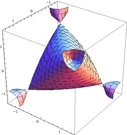
Figure 1. The surface $S_{0.01}$.

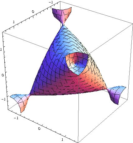
Figure 2. The surface $S_{0.1}$.

Figure 3. The surface $S_{0.2}$.

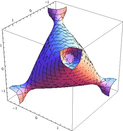
Figure 4. The surface $S_{0.5}$.

Denote by $\ell_{V}$ the line

$$\ell_{V}=\left\{\left(\frac{E-V}{2},\frac{E}{2},1\right):E\in\mathbb{R}\right\}.$$

It is easy to check that $\ell_{V}\subset S_{V}$.

Sütő proved the following central result in [S87].

Theorem 1 (Sütő 1987).

An energy $E$ belongs to the spectrum of $H_{V,\omega}$ if and only if the positive semiorbit of the point $(\frac{E-V}{2},\frac{E}{2},1)$ under iterates of the trace map $T$ is bounded.

It is of course natural to consider the restriction $T_{V}$ of the trace map $T$ to the invariant surface $S_{V}$. That is, $T_{V}:S_{V}\to S_{V}$, $T_{V}=T|_{S_{V}}$. Denote by $\Omega_{V}$ the set of points in $S_{V}$ whose full orbits under $T_{V}$ are bounded. A priori the set of bounded orbits of $T_{V}$ could be different from the non-wandering set of $T_{V}$, but our construction of the Markov partition and analysis of the behavior of $T_{V}$ near singularities show that in our case these two sets do coincide. Notice that this is parallel to the construction of the symbolic coding in [Cas].

Let us recall that an invariant closed set $\Lambda$ of a diffeomorphism $f:M\to M$ is hyperbolic if there exists a splitting of a tangent space $T_{x}M=E^{u}_{x}\oplus E^{u}_{x}$ at every point $x\in\Lambda$ such that this splitting is invariant under $Df$ and the differential $Df$ exponentially contracts vectors from stable subspaces $\{E^{s}_{x}\}$ and exponentially expands vectors from unstable subspaces $\{E^{u}_{x}\}$. A hyperbolic set $\Lambda$ of a diffeomorphism $f:M\to M$ is locally maximal if there exists a neighborhood $U(\Lambda)$ such that

$$\Lambda=\bigcap_{n\in\mathbb{Z}}f^{n}(U).$$

The second central result about the trace map we wish to recall is due to Casdagli; see [Cas].

Theorem 2 (Casdagli 1986).

For $V\geq 16$, the set $\Omega_{V}$ is a locally maximal hyperbolic set of $T_{V}:S_{V}\to S_{V}$. It is homeomorphic to a Cantor set.

2.2. Some Properties of Locally Maximal Hyperbolic Invariant Sets of Surface Diffeomorphisms

Given Theorem 2, several general results apply to the trace map of the strongly coupled Fibonacci Hamiltonian. Let us recall some of these results that yield interesting spectral consequences, which are discussed below.

Consider a locally maximal invariant transitive hyperbolic set $\Lambda\subset M$, $\dim M=2$, of a diffeomorphism $f\in\text{\, \rm Diff\,}^{r}(M),r\geq 1$. We have $\Lambda=\bigcap_{n\in\mathbb{Z}}f^{n}(U(\Lambda))$ for some neighborhood $U(\Lambda)$. Assume also that $\dim E^{u}=\dim E^{s}=1$. Then, the following properties hold.

2.2.1. Stability

There is a neighborhood $\mathcal{U}\subset\text{\, \rm Diff\,}^{1}(M)$ of the map $f$ such that for every $g\in\mathcal{U}$, the set $\Lambda_{g}=\bigcap_{n\in\mathbb{Z}}g(U(\Lambda))$ is a locally maximal invariant hyperbolic set set of $g$. Moreover, there is a homeomorphism $h:\Lambda\to\Lambda_{g}$ that conjugates $f|_{\Lambda}$ and $g|_{\Lambda_{g}}$, that is, the following diagram commutes:

$$\begin{CD}\Lambda @>{f|_{\Lambda}}>{}>\Lambda\\ @V{h}V{}V@V{}V{h}V\\ \Lambda_{g}@>{g|_{\Lambda_{g}}}>{}>\Lambda_{g}\end{CD}$$

2.2.2. Invariant Manifolds

For $x\in\Lambda$ and small $\varepsilon>0$, consider the local stable and unstable sets

$$W^{s}_{\varepsilon}(x)=\{w\in M:d(f^{n}(x),f^{n}(w))\leq\varepsilon\ \ \text{\rm for all}\ \ n\geq 0\},$$

$$W^{u}_{\varepsilon}(x)=\{w\in M:d(f^{n}(x),f^{n}(w))\leq\varepsilon\ \ \text{\rm for all}\ \ n\leq 0\}.$$

If $\varepsilon>0$ is small enough, these sets are embedded $C^{r}$-disks with $T_{x}W^{s}_{\varepsilon}(x)=E^{s}_{x}$ and $T_{x}W^{u}_{\varepsilon}(x)=E^{u}_{x}$. Define the (global) stable and unstable sets as

$$W^{s}(x)=\bigcup_{n\in\mathbb{N}}f^{-n}(W^{s}_{\varepsilon}(x)),\ \ \ W^{u}(x)=\bigcup_{n\in\mathbb{N}}f^{n}(W^{u}_{\varepsilon}(x)).$$

Define also

$$W^{s}(\Lambda)=\bigcup_{x\in\Lambda}W^{s}(x)\ \ \ \text{\rm and}\ \ \ W^{u}(\Lambda)=\bigcup_{x\in\Lambda}W^{u}(x).$$

2.2.3. Invariant Foliations

A stable foliation for $\Lambda$ is a foliation $\mathcal{F}^{s}$ of a neighborhood of $\Lambda$ such that

• for each $x\in\Lambda$, $\mathcal{F}(x)$, the leaf containing $x$, is tangent to $E^{s}_{x}$,

• for each $x$ sufficiently close to $\Lambda$, $f(\mathcal{F}^{s}(x))\subset\mathcal{F}^{s}(f(x))$.

An unstable foliation $\mathcal{F}^{u}$ can be defined in a similar way.

For a locally maximal hyperbolic set $\Lambda\subset M$ of a $C^{1}$-diffeomorphism $f:M\to M$, $\dim M=2$, stable and unstable $C^{0}$ foliations with $C^{1}$-leaves can be constructed [M]. In the case of $C^{2}$-diffeomorphism, $C^{1}$ invariant foliations exist (see, for example, [PT], Theorem 8 in Appendix 1).

2.2.4. Local Hausdorff Dimension and Box Counting Dimension

Consider, for $x\in\Lambda$ and small $\varepsilon>0$, the set $W^{u}_{\varepsilon}(x)\cap\Lambda$. Its Hausdorff dimension does not depend on $x\in\Lambda$ and $\varepsilon>0$, and coincides with its box counting dimension (see [MM, T]):

$$\dim_{H}W^{u}_{\varepsilon}(x)\cap\Lambda=\dim_{B}W^{u}_{\varepsilon}(x)\cap\Lambda.$$

In a similar way,

$$\dim_{H}W^{s}_{\varepsilon}(x)\cap\Lambda=\dim_{B}W^{s}_{\varepsilon}(x)\cap\Lambda.$$

Denote $h^{s}=\dim_{H}W^{s}_{\varepsilon}(x)\cap\Lambda$ and $h^{u}=\dim_{H}W^{u}_{\varepsilon}(x)\cap\Lambda$. We will say that $h^{s}$ and $h^{u}$ are the local stable and unstable Hausdorff dimensions of $\Lambda$.

For properly chosen small $\varepsilon>0$, the sets $W^{u}_{\varepsilon}(x)\cap\Lambda$ and $W^{s}_{\varepsilon}(x)\cap\Lambda$ are dynamically defined Cantor sets (see [PT1] for definitions and proof), and this implies, in particular, that

$$h^{s}<1\ \ \ \text{\rm and}\ \ \ h^{u}<1,$$

see, for example, Theorem 14.5 in [P].

2.2.5. Global Hausdorff Dimension

The Hausdorff dimension of $\Lambda$ is equal to its box counting dimension, and

$$\dim_{H}\Lambda=\dim_{B}\Lambda=h^{s}+h^{u};$$

see [MM, PV].

2.2.6. Continuity of the Hausdorff Dimension

The local Hausdorff dimensions $h^{s}(\Lambda)$ and $h^{u}(\Lambda)$ depend continuously on $f:M\to M$ in the $C^{1}$-topology; see [MM, PV]. Therefore, $\dim_{H}\Lambda_{f}=\dim_{B}\Lambda_{f}=h^{s}(\Lambda_{f})+h^{u}(\Lambda_{f})$ also depends continuously on $f$ in the $C^{1}$-topology. Moreover, for a $C^{r}$ diffeomorphism $f:M\to M$, $r\geq 2$, the Hausdorff dimension of a hyperbolic set $\Lambda_{f}$ is a $C^{r-1}$ function of $f$; see [Ma].

Remark 2.1.

For hyperbolic sets in dimension greater than two, many of these properties do not hold in general; see [P] for more details.

2.3. Implications for the Trace Map and the Spectrum

Due to Theorem 2, for every $V\geq 16$, all the properties from the previous subsection can be applied to the hyperbolic set $\Omega_{\lambda}$ of the trace map $T_{V}:S_{V}\to S_{V}$.

Moreover, the results in [Cas, Section 2] imply the following statement.

Lemma 2.2.

For $V\geq 16$ and every $x\in\Omega_{V}$, the stable manifold $W^{s}(x)$ intersects the line $\ell_{V}$ transversally.

The existence of a $C^{1}$-foliation $\mathcal{F}^{s}$ allows one to locally consider the set $W^{s}(\Omega_{V})\cap\ell_{V}$ as a $C^{1}$-image of the set $W^{u}_{\varepsilon}(x)\cap\Omega_{V}$. Due to Theorem 1, this implies the following properties of the spectrum $\sigma(H_{V,\omega})$ for $V\geq 16$:

Corollary 1.

For $V\geq 16$, the following statements hold:

• The spectrum $\sigma(H_{V,\omega})$ depends continuously on $V$ in the Hausdorff metric.

• For every small $\varepsilon>0$ and every $x\in\sigma(H_{V,\omega})$, we have

  $$\dim_{H}\left((x-\varepsilon,x+\varepsilon)\cap\sigma(H_{V,\omega})\right) =\dim_{B}\left((x-\varepsilon,x+\varepsilon)\cap\sigma(H_{V,\omega})\right)$$

  $$=\dim_{H}\sigma(H_{V,\omega})$$

  $$=\dim_{B}\sigma(H_{V,\omega}).$$

• The Hausdorff dimension $\dim_{H}\sigma(H_{V,\omega})$ is a $C^{\infty}$-function of $V$, and is strictly smaller than one.

2.4. Hyperbolicity of the Trace Map for Small Coupling

We are now in a position to state the main result of this paper.

Theorem 3.

There exists $V_{0}>0$ such that for every $V\in(0,V_{0})$, the following properties hold.

• The non-wandering set $\Omega_{V}\subset S_{V}$ of the map $T_{V}:S_{V}\to S_{V}$ is hyperbolic.

• The non-wandering set $\Omega_{V}\subset S_{V}$ is homeomorphic to a Cantor set, and $T_{V}|_{\Omega_{V}}$ is conjugated to a topological Markov chain $\sigma_{A}:\Sigma^{6}_{A}\to\Sigma^{6}_{A}$ with the matrix

  $$A=\begin{pmatrix}0&0&0&1&1&1\\ 0&0&1&0&1&1\\ 0&0&0&0&1&0\\ 0&0&0&0&0&1\\ 1&0&0&0&0&0\\ 0&1&0&0&0&0\\ \end{pmatrix}.$$

• For every $x\in\Omega_{V}$, the stable manifold $W^{s}(x)$ intersects the line $\ell_{V}$ transversally.

As before, we obtain the following consequences:

Corollary 2.

With $V_{0}>0$ from Theorem 3, the following statements hold for $V\in(0,V_{0})$:

• The spectrum $\sigma(H_{V,\omega})$ depends continuously on $V$ in the Hausdorff metric.

• For every small $\varepsilon>0$ and every $x\in\sigma(H_{V,\omega})$, we have

  $$\dim_{H}\left((x-\varepsilon,x+\varepsilon)\cap\sigma(H_{V,\omega})\right) =\dim_{B}\left((x-\varepsilon,x+\varepsilon)\cap\sigma(H_{V,\omega})\right)$$

  $$=\dim_{H}\sigma(H_{V,\omega})$$

  $$=\dim_{B}\sigma(H_{V,\omega}).$$

• The Hausdorff dimension $\dim_{H}\sigma(H_{V,\omega})$ is a $C^{\infty}$-function of $V$, and is strictly smaller than one.

We expect these properties to be of similar importance in a study of the asymptotic behavior of the fractal dimension of the spectrum as $V\to 0$ as was the case in the large coupling regime.

3. Properties of the Trace Map for $V=0$

Up to this point, we only considered the case $V>0$. Since we will regard the case of small positive $V$ as a small perturbation of the case $V=0$, we will also include the latter case in our considerations. In fact, this section is devoted to the study of this “unperturbed case.”

Denote by $\mathbb{S}$ the part of the surface $S_{0}$ inside of the cube $\{|x|\leq 1,|y|\leq 1,|z|\leq 1\}$. The surface $\mathbb{S}$ is homeomorphic to $S^{2}$, invariant, smooth everywhere except at the four points $P_{1}=(1,1,1)$, $P_{1}=(1,-1,-1)$, $P_{1}=(-1,1,-1)$, and $P_{1}=(-1,-1,1)$, where $\mathbb{S}$ has conic singularities, and the trace map $T$ restricted to $\mathbb{S}$ is a factor of a hyperbolic automorphism of a two torus:

$$\mathcal{A}(\theta,\varphi)=(\theta+\varphi,\theta)\ (\text{\rm mod}\ 1).$$

The semiconjugacy is given by the map

$$F:(\theta,\varphi)\mapsto(\cos 2\pi(\theta+\varphi),\cos 2\pi\theta,\cos 2\pi\varphi).$$

The map $\mathcal{A}$ is hyperbolic, and is given by a matrix $A=\begin{pmatrix}1&1\\ 1&0\\ \end{pmatrix}$ with eigenvalues

$$\mu=\frac{1+\sqrt{5}}{2}\ \ \text{\rm and}\ \ \ -\mu^{-1}=\frac{1-\sqrt{5}}{2}.$$

Let us denote by $\mathbf{v}^{u},\mathbf{v}^{u}\in\mathbb{R}^{2}$ the unstable and stable eigenvectors of $A$:

$$A\mathbf{v}^{u}=\mu\mathbf{v}^{u},\ A\mathbf{v}^{s}=-\mu^{-1}\mathbf{v}^{s},\ \|\mathbf{v}^{u}\|=\|\mathbf{v}^{s}\|=1.$$

Fix some small $\zeta>0$ and define the stable (resp., unstable) cone fields on $\mathbb{R}^{2}$ in the following way:

(1) $$K^{s}_{p} =\{\mathbf{v}\in T_{p}\mathbb{R}^{2}:\mathbf{v}=v^{u}\mathbf{v}^{u}+v^{s}\mathbf{v}^{s},\ |v^{s}|>\zeta^{-1}|v^{u}|\},$$

$$K^{u}_{p} =\{\mathbf{v}\in T_{p}\mathbb{R}^{2}:\mathbf{v}=v^{u}\mathbf{v}^{u}+v^{s}\mathbf{v}^{s},\ |v^{u}|>\zeta^{-1}|v^{s}|\}.$$

These cone fields are invariant:

$$\forall\ \mathbf{v}\in K^{u}_{p}\ \ \ \ A\mathbf{v}\in K^{u}_{A(p)},$$

$$\forall\ \mathbf{v}\in K^{s}_{p}\ \ \ \ A^{-1}\mathbf{v}\in K^{s}_{A^{-1}(p)}.$$

Also, the iterates of the map $A$ expand vectors from the unstable cones, and the iterates of the map $A^{-1}$ expand vectors from the stable cones:

$$\forall\ \mathbf{v}\in K^{u}_{p}\ \ \ \ \forall\ n\in\mathbb{N}\ \ \ \ |A^{n}\mathbf{v}|>\frac{1}{\sqrt{1+\zeta^{2}}}\lambda^{n}|\mathbf{v}|,$$

$$\forall\ \mathbf{v}\in K^{s}_{p}\ \ \ \ \forall\ n\in\mathbb{N}\ \ \ \ |A^{-n}\mathbf{v}|>\frac{1}{\sqrt{1+\zeta^{2}}}\lambda^{n}|\mathbf{v}|.$$

The families of cones $\{K^{s}\}$ and $\{K^{u}\}$ invariant under $\mathcal{A}$ can be also considered on $\mathbb{T}^{2}$.

The differential of the semiconjugacy $F$ sends these cone families to stable and unstable cone families on $\mathbb{S}\backslash\{P_{1},P_{2},P_{3},P_{4}\}$. Let us denote these images by $\{\mathcal{K}^{s}\}$ and $\{\mathcal{K}^{u}\}$.

Lemma 3.1.

The differential of the semiconjugacy $DF$ induces a map of the unit bundle of $\mathbb{T}^{2}$ to the unit bundle of $\mathbb{S}\backslash\{P_{1},P_{2},P_{3},P_{4}\}$. The derivatives of the restrictions of this map to a fiber are uniformly bounded. In particular, the sizes of cones in families $\{\mathcal{K}^{s}\}$ and $\{\mathcal{K}^{u}\}$ are uniformly bounded away from zero.

Proof.

Choose small enough neighborhoods $U_{1}(P_{1}),U_{2}(P_{2}),U_{3}(P_{3})$, and $U_{4}(P_{4})$ in $\mathbb{S}$. The complement

$$\hat{\mathbb{S}}=\mathbb{S}\setminus\Big{(}\bigcup_{j=1}^{4}U_{j}(P_{j})\Big{)}$$

is compact, so $F^{-1}(\hat{\mathbb{S}})$ is also compact, and the action of $DF$ on a fiber of the unit bundle over points of $F^{-1}(\hat{\mathbb{S}})$ has uniformly bounded derivatives.

Due to the symmetries of the trace map (see, for example, [K] for the detailed description of the symmetries of the trace map) and the semiconjugacy $F$, it is enough to consider a neighborhood $U_{1}(P_{1})$. Hence, it is enough to consider the map $F$ in a neighborhood of the point $(0,0)$.

The differential of $F$ has the form

$$DF=-2\pi\begin{pmatrix}\sin 2\pi(\theta+\varphi)&\sin 2\pi(\theta+\varphi)\\ \sin 2\pi\theta&0\\ 0&\sin 2\pi\varphi\\ \end{pmatrix}.$$

If $(\theta,\varphi)$ is in a small neighborhood of $(0,0)$, then

$$DF\sim-4\pi^{2}\begin{pmatrix}\theta+\varphi&\theta+\varphi\\ \theta&0\\ 0&\varphi\\ \end{pmatrix}.$$

Therefore, up to a multiplicative constant and higher order terms, the image of the vector $(1,0)$ under $DF$ is $(\theta+\varphi,\theta,0)$, and the image of the vector $(0,1)$ is $(\theta+\varphi,0,\varphi)$. In order to estimate the derivative of the projective action of $DF$ on a fiber over a point $(\theta,\varphi)$, it is enough to estimate the angle between images of basis vectors, and the ratio of the lengths of the images of these vectors.

If $\alpha$ is the angle between $DF_{(\theta,\varphi)}(1,0)$ and $DF_{(\theta,\varphi)}(0,1)$, then

$$\cos\alpha\sim\frac{(\theta+\varphi)^{2}}{\sqrt{(\theta+\varphi)^{2}+\theta^{2}}\cdot\sqrt{(\theta+\varphi)^{2}+\varphi^{2}}}=\frac{1}{\sqrt{1+\frac{\theta^{2}+\varphi^{2}}{(\theta+\varphi)^{2}}+\frac{\theta^{2}\varphi^{2}}{(\theta+\varphi)^{4}}}}.$$

We have

$$\frac{\theta^{2}+\varphi^{2}}{(\theta+\varphi)^{2}}\geq\frac{1}{2},\ \ \ \text{\rm and}\ \ \ \frac{\theta^{2}\varphi^{2}}{(\theta+\varphi)^{4}}\geq 0,$$

so $\cos\alpha\leq\sqrt{\frac{2}{3}}+0.001<1$ if $(\theta,\varphi)$ is close enough to $(0,0)$.

Now let us estimate the ratio of the lengths of $DF_{(\theta,\varphi)}(1,0)$ and $DF_{(\theta,\varphi)}(0,1)$. Up to higher order terms it is equal to

$$\frac{\sqrt{\varphi^{2}+2\theta^{2}+2\theta\varphi}}{\sqrt{2\varphi^{2}+\theta^{2}+2\theta\varphi}}=\sqrt{\frac{1+2t^{2}+2t}{2+t^{2}+2t}}=\sqrt{\frac{2(t+\frac{1}{2})^{2}+\frac{1}{2}}{(t+1)^{2}+1}},$$

where $t=\frac{\theta}{\varphi}\in\mathbb{R}\cup{\{\infty\}}$, and this function is bounded from above and bounded away from zero. Lemma 3.1 is proved. ∎

4. The Structure of the Trace Map in a Neighborhood of a Singular Point

Due to the symmetries of the trace map it is enough to consider the dynamics of $T$ in a neighborhood of $P_{1}=(1,1,1)$. Let $U\subset\mathbb{R}^{3}$ be a small neighborhood of $P_{1}$ in $\mathbb{R}^{3}$. Let us consider the set $Per_{2}(T)$ of periodic points of $T$ of period 2.

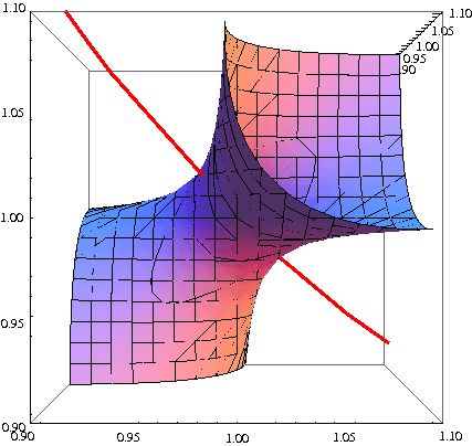
Figure 5. $S_{0.1}$ and $Per_{2}(T)$ near $(1,1,1)$.

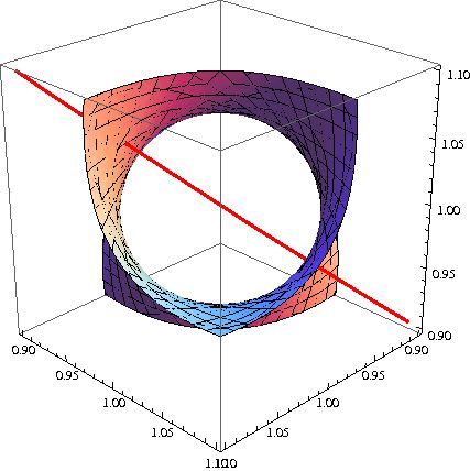
Figure 6. $S_{0.2}$ and $Per_{2}(T)$ near $(1,1,1)$.

Lemma 4.1.

We have

$$Per_{2}(T)=\left\{(x,y,z):x\in(-\infty,\tfrac{1}{2})\cup(\tfrac{1}{2},\infty),\ y=\frac{x}{2x-1},\ z=x\right\}.$$

Proof.

Direct calculation. ∎

Notice that in a neighborhood $U$ the intersection $I\equiv Per_{2}(T)\cap U$ is a smooth curve that is a normally hyperbolic with respect to $T$ (see, for example, [PT], Appendix 1, for the formal definition of normal hyperbolicity). Therefore, the local center-stable manifold $W_{loc}^{cs}(I)$ and the local center-unstable manifold $W^{cu}_{loc}(I)$ defined by

$$W_{loc}^{cs}(I)=\left\{p\in U:T^{n}(p)\in U\ \text{\rm for all}\ n\in\mathbb{N}\right\},$$

$$W_{loc}^{cu}(I)=\left\{p\in U:T^{-n}(p)\in U\ \text{\rm for all}\ n\in\mathbb{N}\right\}$$

are smooth two-dimensional surfaces. Also, the local strong stable manifold $W^{ss}_{loc}(P_{1})$ and the local strong unstable manifold $W^{uu}_{loc}(P_{1})$ of the fixed point $P_{1}$, defined by

$$W^{ss}_{loc}(P_{1})=\left\{p\in W^{cs}_{loc}(I):T^{n}(p)\to P_{1}\ \text{\rm as}\ n\to+\infty\right\},$$

$$W^{uu}_{loc}(P_{1})=\left\{p\in W^{cu}_{loc}(I):T^{-n}(p)\to P_{1}\ \text{\rm as}\ n\to+\infty\right\},$$

are smooth curves.

Let $\Phi:U\to\mathbb{R}^{3}$ be a smooth change of coordinates such that $\Phi(P_{1})=(0,0,0)$ and

• $\Phi(I)$ is a part of the line $\{x=0,z=0\}$;

• $\Phi(W^{cs}_{loc}(I))$ is a part of the plane $\{z=0\}$;

• $\Phi(W^{cu}_{loc}(I))$ is a part of the plane $\{x=0\}$;

• $\Phi(W^{ss}_{loc}(P_{1}))$ is a part of the line $\{y=0,z=0\}$;

• $\Phi(W^{uu}_{loc}(P_{1}))$ is a part of the line $\{x=0,y=0\}$.

Denote $f=\Phi\circ T\circ\Phi^{-1}$.

In this case,

$$Df(0,0,0)=D(\Phi\circ T\circ\Phi^{-1})(0,0,0)=\begin{pmatrix}\lambda^{-1}&0&0\\ 0&-1&0\\ 0&0&\lambda\\ \end{pmatrix},$$

where $\lambda$ is a largest eigenvalue of the differential $DT(P_{1}):T_{P_{1}}\mathbb{R}^{3}\to T_{P_{1}}\mathbb{R}^{3}$,

$$DT(P_{1})=\begin{pmatrix}2&2&-1\\ 1&0&0\\ 0&1&0\\ \end{pmatrix},\ \ \ \lambda=\frac{3+\sqrt{5}}{2}=\mu^{2}.$$

Let us denote $\mathfrak{S}_{V}=\Phi(S_{V})$. Then, away from $(0,0,0)$, the family $\{\mathfrak{S}_{V}\}$ is a smooth family of surfaces, $\mathfrak{S}_{0}$ is diffeomorphic to a cone, contains lines the $\{y=0,z=0\}$ and $\{x=0,y=0\}$, and at each non-zero point on these lines, it has a quadratic tangency with a horizontal or vertical plane; compare Figures 6 and 6.

We will use the variables $(x,y,z)$ for coordinates in $\mathbb{R}^{3}$. For a point $p\in\mathbb{R}^{3}$, we will denote its coordinates by $(x_{p},y_{p},z_{p})$.

In order to study the properties of the map $f$ (i.e., of the map $T$ in a small neighborhood of singularities), we need the following statement.

Proposition 1.

Given $C_{1}>0,C_{2}>0,\lambda>1$, $\varepsilon\in(0,\frac{1}{4})$, and $\eta>0$, there exist $\delta_{0}=\delta_{0}(C_{1},C_{2},\lambda,\varepsilon)$, $N_{0}\in\mathbb{N}$, $N_{0}=N_{0}(C_{1},C_{2},\lambda,\varepsilon,\delta_{0})$, and $C=C(\eta)>0$ such that for any $\delta\in(0,\delta_{0})$, the following holds.

Let $f:\mathbb{R}^{3}\to\mathbb{R}^{3}$ be a $C^{2}$-diffeomorphism such that

• $\|f\|_{C^{2}}\leq C_{1}$;

• The plane $\{z=0\}$ is invariant under iterates of $f$;

• $\|Df(p)-A\|<\delta$ for every $p\in\mathbb{R}^{3}$, where

  $$A=\begin{pmatrix}\lambda^{-1}&0&0\\ 0&1&0\\ 0&0&\lambda\\ \end{pmatrix}$$

  is a constant matrix.

Introduce the following cone field in $\mathbb{R}^{3}$:

(2) $$K_{p}=\{v\in T_{p}\mathbb{R}^{3},\ \mathbf{v}=\mathbf{v}_{xy}+\mathbf{v}_{z}:|\mathbf{v}_{z}|\geq C_{2}\sqrt{|z_{p}|}|\mathbf{v}_{xy}|\}.$$

Given a point $p=(x_{p},y_{p},z_{p})$ such that $0<z_{p}<1$, denote by $N=N(p)$ the smallest integer $N\in\mathbb{N}$ such that $f^{N}(p)$ has $z$-coordinate larger that 1.

If $N(p)\geq N_{0}$ (i.e., if $z_{p}$ is small enough) then

(3) $$|Df^{N}(\mathbf{v})|\geq\lambda^{\frac{N}{2}(1-4\varepsilon)}|\mathbf{v}|\ \ \ \text{for any }\ \ \mathbf{v}\in K_{p},$$

and if $Df^{N}(\mathbf{v})=\mathbf{u}=\mathbf{u}_{xy}+\mathbf{u}_{z}$, then

(4) $$|\mathbf{u}_{xy}|<2\delta^{1/2}|\mathbf{u}_{z}|.$$

Moreover, if $|\mathbf{v}_{z}|\geq\eta|\mathbf{v}_{xy}|$ then

(5) $$|Df^{k}(\mathbf{v})|\geq C\lambda^{\frac{k}{2}(1-4\varepsilon)}|\mathbf{v}|\ \ \ \text{for each }\ \ k=1,2,\ldots,N.$$

Returning to our specific situation at hand, if, for a given $\delta$, the neighborhood $U$ is small enough, then at every point $P\in U$ the differential $D(\Phi\circ T\circ\Phi^{-1})(P)$ satisfies the condition (iii) of Proposition 1. Also, since the tangency of $\mathfrak{S}_{0}$ with the horizontal plane is quadratic, there exists $C_{2}>0$ such that every vector tangent to $\mathfrak{S}_{0}$ from the cone $D\Phi(\mathcal{K}^{u})$ also belongs to the cone (2). The same holds for vectors tangent to $\mathfrak{S}_{V}$ from continuations of cones $D\Phi(\mathcal{K}^{u})$ if $V$ is small enough. Therefore, Proposition 1 can be applied to all those vectors.

We postpone the proof of Proposition 1 to Section 6 and first show how to use it to prove Theorem 3.

5. Proof of Theorem 3 Assuming Proposition 1

In order to prove the hyperbolicity of $\Omega_{V}$ we construct only the unstable cone field and prove the unstable cone condition. Due to the symmetry of the trace map, the stable cones can be constructed in the same way.

Let $U^{\prime}$ be a neighborhood of $\{P_{1},P_{2},P_{3},P_{4}\}$ where the results of the previous section can be applied. Since $\mathbb{S}\backslash U^{\prime}$ is compact, $F^{-1}(\mathbb{S}\backslash U^{\prime})$ is also compact. Denote

$$\widetilde{C}=2\max_{p\in\mathbb{S}\backslash U^{\prime}}\left\{\|DF^{-1}(p)\|,\|DF(F^{-1}(p))\|\right\}<\infty.$$

Take any $p\in\mathbb{S}\backslash U^{\prime}$ and any $\mathbf{v}\in T_{p}\mathbb{S},\mathbf{v}\in\mathcal{K}^{u}.$ If $T^{n}(p)\in\mathbb{S}\backslash U^{\prime}$, then

(6) $$\|DT^{n}(\mathbf{v})\|=\|D(F\circ\mathcal{A}^{n}\circ F^{-1})(\mathbf{v})\|\geq\widetilde{C}^{-2}\mu^{n}\|\mathbf{v}\|.$$

Fix a small $\varepsilon>0$ and $n^{*}\in\mathbb{N}$ such that $\widetilde{C}^{-2}\mu^{n^{*}}\geq\mu^{n^{*}(1-\varepsilon)}.$

Lemma 5.1.

There exists a neighborhood $U^{*}\subset U^{\prime}$ of the singular set $\{P_{1},P_{2},P_{3},P_{4}\}$ such that if $p\not\in U^{*}$ but $T^{-1}(p)\in U^{*}$, and $n_{0}$ is the smallest positive integer such that $T^{n_{0}}(p)\in U^{*}$, then the finite orbit $\{p,T(p),\ldots,T^{n_{0}-1}(p)\}$ contains at least $n^{*}$ points outside of $U^{\prime}$.

Proof.

Take a point $p_{1}\in W^{uu}_{loc}(P_{1})\subset U$, denote $p_{2}=T(p_{1})$, and consider the closed arc $J\subset W^{uu}(P_{1})$ between points $p_{1}$ and $p_{2}$. For any point $p\in J$, denote by $m(p)$ the smallest number $m\in\mathbb{N}$ such that the finite orbit $\{p,T(p),\ldots,T^{m}(p)\}$ contains $n^{*}$ points outside of $\overline{U^{\prime}}$. Notice that the function $m(p)$ is upper semi-continuous, and therefore (due to compactness of $J$) bounded. Let $M\in\mathbb{N}$ be an upper bound. The set $\bigcup_{i=0}^{M}T^{i}(J)$ is compact and does not contain the singularities $P_{1},P_{2},P_{3}$ and $P_{4}$. Therefore, there exists $\xi>0$ so small that if $\text{\rm dist}(q,J)<\xi$, then the distance between any of the first $M$ iterates of $q$ and any of the points $P_{1},P_{2},P_{3},P_{4}$ is greater than $\xi$, and the finite orbit $\{q,T(q),\ldots,T^{M}(q)\}$ contains at least $n^{*}$ points outside of $\overline{U^{\prime}}$. Now take $\xi^{\prime}>0$ so small that any point in $\xi^{\prime}$-neighborhood of $P_{1}$ whose orbit follows $W^{uu}(P_{1})$ towards $p_{1}$ hits the $\xi$-neighborhood of $J$ before leaving $U^{\prime}$. Now we can take the $\xi^{\prime}$-neighborhood of the set $P_{1},P_{2},P_{3},P_{4}$ as $U^{*}$. ∎

For small $V$, denote by $\mathbb{S}_{V,U^{*}}$ the bounded component of $S_{V}\backslash U^{*}$. The family $\{\mathbb{S}_{V,U^{*}}\}_{V\in[0,V_{0})}$ of surfaces with boundary depends smoothly on the parameter and has uniformly bounded curvature. For small $V$, a projection $\pi_{V}:\mathbb{S}_{V,U^{*}}\to\mathbb{S}$ is defined. The map $\pi_{V}$ is smooth, and if $p\in\mathbb{S}$, $q\in\mathbb{S}_{V,U^{*}}$, and $\pi_{V}(q)=p$, then $T_{p}\mathbb{S}$ and $T_{q}S_{V}$ are close. Denote by $\mathcal{K}_{V}^{u}$ (resp., $\mathcal{K}_{V}^{s}$) the image of the cone $\mathcal{K}^{u}$ (resp., $\mathcal{K}^{s}$) under the differential of $\pi_{V}^{-1}$.

Our choice of $n^{*}$ guarantees that the following statement holds.

Lemma 5.2.

There exists $V_{0}>0$ such that for every $V\in[0,V_{0})$, the following holds: if $\{q,T(q),T^{2}(q),\ldots,T^{n}(q)\}\subset\mathbb{S}_{V,U^{*}}$, $\mathbf{v}\in\mathcal{K}_{V}^{u}\subset T_{q}S_{V}$, $q,T^{n}(q)\in\mathbb{S}_{V,U^{\prime}}$, and $n\geq n^{*}$, then

$$\|DT^{n}(\mathbf{v})\|\geq\mu^{n(1-2\varepsilon)}\|\mathbf{v}\|.$$

Lemma 5.3.

There exist $V_{0}>0$ and $C>0$ such that for any $V\in[0,V_{0})$, we have that if $q\in\mathbb{S}_{V,U^{\prime}}$, $\mathbf{v}\in\mathcal{K}_{V}^{u}\subset T_{q}S_{V}$, and $T^{n}(q)\in\mathbb{S}_{V,U^{\prime}}$, then

$$\|DT^{n}(\mathbf{v})\|\geq C\mu^{n(1-4\varepsilon)}\|\mathbf{v}\|.$$

Proof.

Let us split the orbit $\{q,T(q),T^{2}(q),\ldots,T^{n}(q)\}$ into several intervals

$$\{q,T(q),T^{2}(q),\ldots,T^{k_{1}-1}(q)\},\{T^{k_{1}}(q),\ldots,T^{k_{2}-1}(q)\},\ldots,\{T^{k_{s}}(q),\ldots,T^{n}(q)\}$$

in such a way that the following properties hold:

1. for each $i=1,2,\ldots,s$, the points $T^{k_{i}-1}(q)$ and $T^{k_{i}}(q)$ are outside of $U^{\prime}$;

2. if $\{T^{k_{i}}(q),\ldots,T^{k_{i+1}-1}(q)\}\cap U^{*}\neq\emptyset$, then $\{T^{k_{i}+1}(q),\ldots,T^{k_{i+1}-2}(q)\}\subset U^{\prime}$;

3. for each $i=1,2,\ldots,s-1$, we have either $k_{i+1}-k_{i}\geq n^{*}$ or $\{T^{k_{i}}(q),\ldots,T^{k_{i+1}-1}(q)\}\cap U^{*}\neq\emptyset$.

Such a splitting exists due to the choice of $U^{*}$ above.

The following lemma is a consequence of Lemma 3.1 and property (4) from Proposition 1.

Lemma 5.4.

Suppose $q\in\mathbb{S}_{V,U^{\prime}}$, $\mathbf{v}\in\mathcal{K}_{V}^{u}\subset T_{q}S_{V}$, $T(q)\in U^{\prime}$, and $l\in\mathbb{N}$ is the smallest number such that $T^{l}(q)\not\in U^{\prime}$. If $l$ is large enough and $V$ is small enough, then

$$DT^{l}(q)(\mathbf{v})\in\mathcal{K}_{V}^{u}\subset T_{T^{l}(q)}S_{V}.$$

Apply Lemma 5.4 to those intervals in the splitting that are contained in $U^{\prime}$. Notice that largeness of $l$ can be provided by the choice of $U^{*}$. Together with Proposition 1 applied to these intervals, and Lemma 5.2 applied to intervals that do not intersect $U^{*}$, this guarantees uniform expansion of $\mathbf{v}$. The first and the last interval may have length greater than $n^{*}$, and then Lemma 5.2 can be applied, or smaller than $n^{*}$, but then taking a small enough constant $C$ (say, $C<\widetilde{C}^{-2}$) will compensate for the lack of uniform expansion on these intervals. Lemma 5.3 is proved. ∎

For every small $V>0$, there exists $\eta_{V}>0$ ($\eta_{V}\to 0$ as $V\to 0$) such that if $p\not\in U^{\prime}$, $T(p)\in U^{\prime}$, and $\mathbf{v}\in\mathcal{K}_{V}^{u}(p)$, then for the vector $\mathbf{w}\equiv D\Phi^{-1}(p)(\mathbf{v})$, $\mathbf{w}=\mathbf{w}_{z}+\mathbf{w}_{xy}$, we have $|\mathbf{w}_{z}|\geq\eta_{V}|\mathbf{w}_{xy}|$. An application of Proposition 1 together with Lemma 5.3 proves uniform expansion of vectors from $\mathcal{K}_{V}^{u}$. Due to the symmetries of the trace map, all vectors from $\mathcal{K}_{V}^{s}$ are expanded by iterates of $T^{-1}$. Thus, hyperbolicity of the set $\Omega_{V}$ follows and Theorem 3 (i) is proved.

The Markov partition for $T|_{\mathbb{S}}$ (i.e., for $V=0$) was presented explicitly by Casdagli in [Cas, Section 2]; compare Figure 7.

Figure 7. The Markov partition for $T|_{\mathbb{S}}$.

Since the Markov partition is formed by finite pieces of strong stable and strong unstable manifolds of the periodic points of $T$ and these manifolds depend smoothly on the parameter $V$, there exists a Markov partition for $\Omega_{V}$ with the same matrix as for $V=0$ (see [PT, Appendix 2] for more details on Markov partitions for 2-dimensional hyperbolic maps). This establishes Theorem 3 (ii).

Lemma 5.5.

If $V$ is small enough, then the line $\ell_{V}$ is transversal to the cone field $\mathcal{K}_{V}^{s}$.

Proof.

For $V=0$ and small enough $\zeta$ in (1), this is true since $F^{-1}(l_{0})=\{\theta=-\varphi\}$, and the vector $(1,-1)$ is not an eigenvector of $A$. Therefore this is also true for every sufficiently small $V$ by continuity. ∎

In order to show that $\ell_{V}$ is also transversal to the stable manifolds of $\Omega_{V}$ inside of $U^{*}$, let us consider the rectifying coordinates $\Phi:U^{*}\to\mathbb{R}^{3}$ again and define the central-unstable cone field in $\Phi(U^{*})$:

$$K_{p}^{cu}=\left\{\mathbf{v}\in T_{p}\mathbb{R}^{3},\mathbf{v}=\mathbf{v}_{x}+\mathbf{v}_{yz}:|\mathbf{v}_{yz}|>\zeta^{-1}|\mathbf{v}_{x}|\right\}.$$

Since $\Phi(l_{0})$ is transversal to the plane $\{x=0\}$, the curve $\Phi(\ell_{V})$ is transversal to this invariant cone field if $\zeta,V$, and $U^{*}$ are small enough. Every stable manifold of $\Omega_{V}$ in the rectifying coordinates is tangent to this central-unstable cone field, and together with Lemma 5.5 this implies that $\ell_{V}$ is transversal to stable manifolds of $\Omega_{V}$. This shows Theorem 3 (iii) and hence concludes the proof of Theorem 3.

6. Proof of Proposition 1

6.1. Properties of the Recurrent Sequences

In this subsection we formulate and prove several lemmas on recurrent sequences that will be used in the next subsection to prove Proposition 1.

Lemma 6.1.

Given $C_{1}>0$, $C_{2}>0$, $\lambda>1$, and $\varepsilon\in(0,\frac{1}{4})$, there exist $\delta_{0}=\delta_{0}(C_{1},C_{2},\lambda,\varepsilon)$ and $N_{0}\in\mathbb{N}$, $N_{0}=N_{0}(C_{1},C_{2},\lambda,\varepsilon,\delta_{0})$, such that for every $\delta\in(0,\delta_{0})$ and every $N\geq N_{0}$, the following holds. Suppose that the sequences $\{d_{i}\}_{i=0}^{N}$, $\{D_{i}\}_{i=0}^{N}$ are defined by the initial conditions

(9) $$\left\{\begin{array}[]{ll}d_{0}=1\\ D_{0}\geq C_{2}\frac{1}{(\lambda+\delta)^{N/2}},\end{array}\right.$$

and recurrence relations

(12) $$\left\{\begin{array}[]{ll}d_{k+1}=(1+2\delta)d_{k}+\delta D_{k},\\ D_{k+1}=(\lambda-\delta)D_{k}-C_{1}b_{k}d_{k},\end{array}\right.$$

where

$$b_{k}=(\lambda-\delta)^{-N+k}.$$

Then

$$\left\{\begin{array}[]{ll}d_{N}\leq 2\delta^{1/2}D_{N}\\ D_{N}\geq D_{0}\lambda^{N(1-\varepsilon)}>\lambda^{\frac{N}{2}(1-4\varepsilon)}.\end{array}\right.$$

Remark 6.2.

Notice that Lemma 6.1 implies also that

$$\frac{d_{N}}{D_{N}}\leq 2\delta^{1/2}.$$

This inequality will allow us to obtain a small cone (of size of order $\delta^{1/2}$) where the image of a vector after leaving a neighborhood of a singularity is located.

Proof of Lemma 6.1..

Let us denote

$$\Lambda_{-}=\lambda^{1-\varepsilon},\ \ \ \Lambda_{+}=\lambda^{1+\varepsilon}.$$

If $\delta$ is small enough, then $1<\Lambda_{-}<\lambda-\delta<\lambda+\delta<\Lambda_{+}$. We will prove by induction that

(15) $$\left\{\begin{array}[]{ll}d_{k}\leq(1+2\delta+\delta^{1/2})\max\{d_{k-1},\delta^{1/2}D_{k-1}\}\\ D_{k}\geq\Lambda_{-}D_{k-1}\geq\Lambda_{-}^{k}D_{0}.\end{array}\right.$$

It is clear that these inequalities for $k=N$ imply Lemma 6.1.

Let us first check the base of induction. If $N$ is large, then $D_{0}<1$, so $\max\{d_{0},\delta^{1/2}D_{0}\}=d_{0}=1$. So we have

$$d_{1}=(1+2\delta)d_{0}+\delta D_{0}<1+3\delta<(1+2\delta+\delta^{1/2})d_{0}.$$

This is the first inequality in (15) for $k=1$.

Also we have

$$D_{1} =(\lambda-\delta)D_{0}-C_{1}b_{0}d_{0}$$

$$=(\lambda-\delta)D_{0}\left(1-\frac{C_{1}b_{0}d_{0}}{D_{0}}\right)$$

$$\geq(\lambda-\delta)D_{0}\left(1-\frac{C_{1}(\lambda+\delta)^{N/2}}{C_{2}(\lambda-\delta)^{N}}\right)$$

$$>(\lambda-\delta)D_{0}\left(1-\frac{C_{1}\Lambda_{+}^{N/2}}{C_{2}\Lambda_{-}^{N}}\right)$$

$$=(\lambda-\delta)D_{0}\left(1-\frac{C_{1}}{C_{2}}\lambda^{-\frac{N}{2}(1-3\varepsilon)}\right),$$

and since $(\lambda-\delta)\left(1-\frac{C_{1}}{C_{2}}\lambda^{-\frac{N}{2}(1-3\varepsilon)}\right)>\Lambda_{-}$ if $N$ is large enough, we have $D_{1}>\Lambda_{-}D_{0}$. We checked the base of induction.

We proceed to proving the induction step. Assume that for some $k$, the inequalities (15) hold. Let us show that these inequalities also hold for $k+1$. We have

$$d_{k+1}=(1+2\delta)d_{k}+\delta D_{k}.$$

If $\delta^{1/2}D_{k}\leq d_{k}$, then

$$d_{k+1} \leq(1+2\delta)d_{k}+\delta^{1/2}d_{k}$$

$$=(1+2\delta+\delta^{1/2})d_{k}$$

$$=(1+2\delta+\delta^{1/2})\max\{d_{k-1},\delta^{1/2}D_{k-1}\}.$$

If $\delta^{1/2}D_{k}>d_{k}$, then

$$d_{k+1} \leq(1+2\delta)\delta^{1/2}D_{k}+\delta D_{k}$$

$$=\delta^{1/2}D_{k}(1+2\delta+\delta^{1/2})$$

$$=(1+2\delta+\delta^{1/2})\max\{d_{k-1},\delta^{1/2}D_{k-1}\}.$$

In order to estimate $D_{k+1}$, we need more information on $\{d_{i}\}_{i=0}^{k}$.

Lemma 6.3.

Assume that $k^{*}\leq N$ and (15) holds for all $k=1,\ldots,k^{*}$. Assume also that for $k=1,2,\ldots,l-1$, we have $\delta^{1/2}D_{k}\leq d_{k}$ and $\delta^{1/2}D_{l}>d_{l}$. Then, $\delta^{1/2}D_{k}>d_{k}$ for every $k=l,l+1,\ldots,k^{*}$.

Proof.

If $\delta$ is small enough, $1+2\delta+\delta^{1/2}<\Lambda_{-}$. Therefore, if $\delta^{1/2}D_{l}>d_{l}$, then

$$d_{l+1} =(1+2\delta)d_{l}+\delta D_{l}$$

$$<(1+2\delta+\delta^{1/2})\delta^{1/2}D_{l}$$

$$<\Lambda_{-}\delta^{1/2}D_{l}$$

$$\leq\delta^{1/2}D_{l+1}.$$

In the same way, $d_{l+2}<\delta^{1/2}D_{l+2}$, and so on. ∎

Notice that Lemma 6.3 immediately implies the following statement.

Lemma 6.4.

Assume that $k^{*}\leq N$ and (15) holds for all $k=1,\ldots,k^{*}$. If $d_{k}\geq\delta^{1/2}D_{k}$ for some $k\in\{1,2,\ldots,k^{*}\}$, then $d_{k}\leq(1+2\delta+\delta^{1/2})^{k}$.

Now let us estimate $D_{k+1}$. If $d_{k}<\delta^{1/2}D_{k}$, then

$$D_{k+1} =(\lambda-\delta)D_{k}\left(1-\frac{C_{1}b_{k}d_{k}}{(\lambda-\delta)D_{k}}\right)$$

$$\geq(\lambda-\delta)D_{k}\left(1-\left(\frac{C_{1}}{\lambda-\delta}\right)\frac{\delta^{1/2}}{(\lambda-\delta)^{N-k}}\right)$$

$$>(\lambda-\delta)D_{k}(1-C_{1}\delta^{1/2})$$

$$>\Lambda_{-}D_{k}$$

if $\delta$ is small enough.

If $d_{k}\geq\delta^{1/2}D_{k}$, then due to Lemma 6.4, we have $d_{k}\leq(1+2\delta+\delta^{1/2})^{k}$, and hence

$$D_{k+1} =(\lambda-\delta)D_{k}\left(1-\frac{C_{1}b_{k}d_{k}}{(\lambda-\delta)D_{k}}\right)$$

$$\geq(\lambda-\delta)D_{k}\left(1-\left(\frac{C_{1}}{\lambda-\delta}\right)\frac{(1+2\delta+\delta^{1/2})^{k}}{\Lambda_{-}^{k}D_{0}(\lambda-\delta)^{N-k}}\right)$$

$$\geq(\lambda-\delta)D_{k}\left(1-\left(\frac{C_{1}}{C_{2}(\lambda-\delta)}\right)\frac{(1+2\delta+\delta^{1/2})^{k}(\lambda+\delta)^{N/2}}{\Lambda_{-}^{k}(\lambda-\delta)^{N-k}}\right)$$

$$\geq(\lambda-\delta)D_{k}\left(1-\left(\frac{C_{1}}{C_{2}(\lambda-\delta)}\right)\frac{(1+2\delta+\delta^{1/2})^{k}\Lambda_{+}^{N/2}}{\Lambda_{-}^{k}\Lambda_{-}^{N-k}}\right)$$

$$\geq(\lambda-\delta)D_{k}\left(1-\left(\frac{C_{1}}{C_{2}(\lambda-\delta)}\right)\frac{(1+2\delta+\delta^{1/2})^{k}\lambda^{\frac{N}{2}(1+\varepsilon)}}{\lambda^{N(1-\varepsilon)}}\right)$$

$$\geq(\lambda-\delta)D_{k}\left(1-\left(\frac{C_{1}}{C_{2}(\lambda-\delta)}\right)(1+2\delta+\delta^{1/2})^{k}\lambda^{-\frac{N}{2}(1-3\varepsilon)}\right)$$

$$>\Lambda_{-}D_{k}$$

if $N$ is large enough. This concludes the proof of Lemma 6.1. ∎

Lemma 6.5.

Given $C_{1}>0$, $C_{2}>0$, $\lambda>1$, and $\varepsilon\in(0,\frac{1}{4})$, there exist $\delta_{0}=\delta_{0}(C_{1},C_{2},\lambda,\varepsilon)$ and $N_{0}\in\mathbb{N}$, $N_{0}=N_{0}(C_{1},C_{2},\lambda,\varepsilon,\delta_{0})$, such that for every $\delta\in(0,\delta_{0})$ and every $N\geq N_{0}$, the following holds. Assume that the sequences $\{a_{k}\}_{k=0}^{N}$ and $\{A_{k}\}_{k=0}^{N}$ have the following properties:

(18) $$\left\{\begin{array}[]{ll}a_{0}=1\\ A_{0}\geq C_{2}\sqrt{\widetilde{b}_{0}}>0,\end{array}\right.$$

and for $k=0,2,\ldots,N-1$

(21) $$\left\{\begin{array}[]{ll}a_{k+1}\leq(1+2\delta)a_{k}+\delta A_{k},\\ A_{k+1}\geq(\lambda-\delta)A_{k}-C_{1}\widetilde{b}_{k}a_{k},\end{array}\right.$$

where the sequence $\widetilde{b_{k}}$ has the properties:

$$0<\widetilde{b}_{0}<\widetilde{b}_{1}<\ldots<\widetilde{b}_{N-1}<1\leq\widetilde{b}_{N},$$

and for all $k=0,2,\ldots,N-1$

$$(\lambda-\delta)\widetilde{b}_{k}\leq\widetilde{b}_{k+1}\leq(\lambda+\delta)\widetilde{b}_{k}.$$

Then,

$$\left\{\begin{array}[]{ll}a_{N}\leq 2\delta^{1/2}A_{N}\\ A_{N}\geq\lambda^{N(1-\varepsilon)}A_{0}>\lambda^{\frac{N}{2}(1-4\varepsilon)}.\end{array}\right.$$

Proof.

Consider the sequences $\{d_{k}\}$ and $\{D_{k}\}$ defined by (9) and (12), where we take $D_{0}=A_{0}$. If we prove that for all $k=0,1,\ldots,N$

(24) $$\left\{\begin{array}[]{ll}A_{k}\geq D_{k}\\ \frac{A_{k}}{a_{k}}\geq\frac{D_{k}}{d_{k}},\end{array}\right.$$

then the required inequalities follow from Lemma 6.1.

We will prove (24) by induction. The base of induction ($k=0$) is provided by our choice of $D_{0}$. Let us turn to the induction step. If (24) holds for some $k$, then

$$\frac{A_{k+1}}{a_{k+1}} \geq\frac{(\lambda-\delta)A_{k}-C_{1}\widetilde{b}_{k}a_{k}}{(1+2\delta)a_{k}+\delta A_{k}}$$

$$=(\lambda-\delta)\delta^{-1}-\frac{(1+2\delta)(\lambda-\delta)\delta^{-1}+C_{1}\widetilde{b}_{k}}{(1+2\delta)+\delta\frac{A_{k}}{a_{k}}}$$

$$\geq(\lambda-\delta)\delta^{-1}-\frac{(1+2\delta)(\lambda-\delta)\delta^{-1}+C_{1}{b_{k}}}{(1+2\delta)+\delta\frac{D_{k}}{d_{k}}}$$

$$=\frac{D_{k+1}}{d_{k+1}}.$$

Also,

$$A_{k+1} \geq(\lambda-\delta)A_{k}-C_{1}b_{k}a_{k}$$

$$=A_{k}\left((\lambda-\delta)-C_{1}\widetilde{b}_{k}\frac{a_{k}}{A_{k}}\right)$$

$$\geq D_{k}\left((\lambda-\delta)-C_{1}{b_{k}}\frac{d_{k}}{D_{k}}\right)$$

$$=D_{k+1}.$$

Lemma 6.5 is proved. ∎

6.2. Expansion of Vectors From Large Cones

Finally, we come to the

Proof of Proposition 1..

Take $\mathbf{v}\in K_{p}$. If $|\mathbf{v}_{z}|>|\mathbf{v}_{xy}|$, then the required inequalities follow just from the condition (iii). Therefore, we can assume that $|\mathbf{v}_{xy}|\geq|\mathbf{v}_{z}|$, and normalize the vector $\mathbf{v}$ assuming that $|\mathbf{v}_{xy}|=1$.

Denote

$$Df(p)=\begin{pmatrix}\nu(p)&m_{1}(p)&t_{1}(p)\\ m_{2}(p)&e(p)&t_{2}(p)\\ s_{1}(p)&s_{2}(p)&\lambda(p)\\ \end{pmatrix}.$$

Given a vector $\mathbf{v}\in K_{p}$, denote $\mathbf{v}^{\prime}=Df(p)(\mathbf{v})$, $\mathbf{v}^{\prime}=\mathbf{v}^{\prime}_{xy}+\mathbf{v}^{\prime}_{z}$, $\mathbf{v}^{\prime}_{xy}=\mathbf{v}^{\prime}_{x}+\mathbf{v}^{\prime}_{y}$. We have

$$Df(p)(\mathbf{v})=\begin{pmatrix}\nu(p)&m_{1}(p)&t_{1}(p)\\ m_{2}(p)&e(p)&t_{2}(p)\\ s_{1}(p)&s_{2}(p)&\lambda(p)\\ \end{pmatrix}\begin{pmatrix}\mathbf{v}_{x}\\ \mathbf{v}_{y}\\ \mathbf{v}_{z}\\ \end{pmatrix}=\begin{pmatrix}\nu(p)\mathbf{v}_{x}+m_{1}(p)\mathbf{v}_{y}+t_{1}(p)\mathbf{v}_{z}\\ m_{2}(p)\mathbf{v}_{x}+e(p)\mathbf{v}_{y}+t_{2}(p)\mathbf{v}_{z}\\ s_{1}(p)\mathbf{v}_{x}+s_{2}(p)\mathbf{v}_{y}+\lambda(p)\mathbf{v}_{z}\\ \end{pmatrix}$$

The conditions (i)–(iii) of Proposition 1 imply that $|\nu(p)|\leq\lambda^{-1}+\delta$, $|m_{1}(p)|,|m_{2}(p)|,|t_{1}(p)|,|t_{2}(p)|\leq\delta$, and $|\lambda(p)|\geq\lambda-\delta$. Also, if $p$ belongs to the plane $\{z=0\}$, then $s_{1}(p)=s_{2}(p)=0$. Since $\|f\|_{C^{2}}\leq C_{1}$, for arbitrary $p$, we have $|s_{1}(p)|,|s_{2}(p)|\leq C_{1}z_{p}$.

Let us use the norm $\|\mathbf{v}\|=|\mathbf{v}_{x}|+|\mathbf{v}_{y}|+|\mathbf{v}_{z}|$. Then we have

$$\|\mathbf{v}_{xy}^{\prime}\|\leq(1+2\delta)\|\mathbf{v}_{xy}\|+\delta\|\mathbf{v}_{z}\|,$$

$$\|\mathbf{v}_{z}^{\prime}\|\geq(\lambda-\delta)\|\mathbf{v}_{z}\|-C_{1}z_{p}\|\mathbf{v}_{xy}\|.$$

Denote by $\widetilde{b}_{k}$ the $z$-coordinate of $f^{k}(p)$, by $A_{k}$ the $z$-component of the vector $Df^{k}(p)(\mathbf{v})$, and by $a_{k}$ the $xy$-component of $Df^{k}(p)(\mathbf{v})$. Applying Lemma 6.5 we get (3), and (4) follows from Remark 6.2.

Now if $A_{0}=|\mathbf{v}_{z}|\geq\eta$, then (applying Lemma 6.1 for $D_{0}=\eta$) from (24) and (15), we have

$$|Df^{k}(p)(\mathbf{v})|\geq A_{k}\geq D_{k}\geq\Lambda_{-}^{k}D_{0}\geq\lambda^{\frac{k}{2}(1-\varepsilon)}\eta>\frac{1}{2}\lambda^{\frac{k}{2}(1-\varepsilon)}\eta|\mathbf{v}|>C\lambda^{\frac{k}{2}(1-4\varepsilon)}|\mathbf{v}|$$

for every $k=1,2,\ldots,N$, where $C=\frac{1}{2}\eta$. Proposition 1 is proved. ∎

References

- [1]
- [AYa] V. M. Alekseev, M. V. Yakobson, Symbolic dynamics and hyperbolic dynamic systems, Phys. Rep. 75 (1981), 287–325.
- [BGJ] M. Baake, U. Grimm, D. Joseph, Trace maps, invariants, and some of their applications, Internat. J. Modern Phys. B 7 (1993), 1527–1550.
- [BR] M. Baake, J. Roberts, The dynamics of trace maps, in Hamiltonian Mechanics (Toruń, 1993), 275–285, NATO Adv. Sci. Inst. Ser. B Phys. 331, Plenum, New York, 1994.
- [Cas] M. Casdagli, Symbolic dynamics for the renormalization map of a quasiperiodic Schrödinger equation, Comm. Math. Phys. 107 (1986), 295–318.
- [Can] S. Cantat, Bers and Hénon, Painlevé and Schrödinger, arXiv:0711.1727v2 [math.CA].
- [D00] D. Damanik, Gordon-type arguments in the spectral theory of one-dimensional quasicrystals, in Directions in Mathematical Quasicrystals, 277–305, CRM Monogr. Ser. 13, Amer. Math. Soc., Providence, RI, 2000.
- [D07] D. Damanik, Strictly ergodic subshifts and associated operators, in Spectral Theory and Mathematical Physics: a Festschrift in Honor of Barry Simon’s 60th Birthday, 505–538, Proc. Sympos. Pure Math. 76, Part 2, Amer. Math. Soc., Providence, RI, 2007.
- [DEGT] D. Damanik, M. Embree, A. Gorodetski, S. Tcheremchantsev, The fractal dimension of the spectrum of the Fibonacci Hamiltonian, Commun. Math. Phys. 280 (2008), 499–516.
- [DL] D. Damanik, D. Lenz, Uniform spectral properties of one-dimensional quasicrystals, I. Absence of eigenvalues, Commun. Math. Phys. 207 (1999), 687–696.
- [DT] D. Damanik and S. Tcheremchantsev, Upper bounds in quantum dynamics, J. Amer. Math. Soc. 20 (2007), 799–827.
- [HM] S. Humphries, A. Manning, Curves of fixed points of trace maps, Ergod. Th. & Dynam. Sys. 27 (2007), 1167–1198.
- [K] L. P. Kadanoff, Analysis of cycles for a volume preserving map, unpublished manuscript.
- [KKT] M. Kohmoto, L. P. Kadanoff, C. Tang, Localization problem in one dimension: mapping and escape, Phys. Rev. Lett. 50 (1983), 1870–1872.
- [LW] Q.-H. Liu, Z.-Y. Wen, Hausdorff dimension of spectrum of one-dimensional Schrödinger operator with Sturmian potentials, Potential Anal. 20 (2004), 33–59.
- [M] W. de Melo, Structural stability of diffeomorphisms on two-manifolds, Invent. Math. 21 (1973), 233–246.
- [Ma] R. Mané, The Hausdorff dimension of horseshoes of diffeomorphisms of surfaces, Bol. Soc. Brasil. Mat. (N.S.) 20 (1990), 1–24.
- [MM] A. Manning, H. McCluskey, Hausdorff dimension for horseshoes, Ergodic Theory Dynam. Systems 3 (1983), 251–261.
- [OPRSS] S. Ostlund, R. Pandit, D. Rand, H. Schellnhuber, and E. Siggia, One-dimensional Schrödinger equation with an almost periodic potential, Phys. Rev. Lett. 50 (1983), 1873–1877.
- [P] Ya. Pesin, Dimension Theory in Dynamical Systems, Chicago Lectures in Mathematics Series, 1997.
- [PT] J. Palis, F. Takens, Hyperbolicity and Sensitive Chaotic Dynamics at Homoclinic Bifurcations, Cambridge University Press, 1993.
- [PT1] J. Palis, F. Takens, Homoclinic bifurcations and hyperbolic dynamics, 16o Colo’quio Brasileiro de Matema’tica. [16th Brazilian Mathematics Colloquium] Instituto de Matema’tica Pura e Aplicada (IMPA), Rio de Janeiro, 1987.
- [PV] J. Palis, M. Viana, On the continuity of the Hausdorff dimension and limit capacity for horseshoes, Dynamical Systems, Lecture Notes in Mathematics 1331 (1988), 150–160.
- [Ra] L. Raymond, A constructive gap labelling for the discrete Schrödinger operator on a quasiperiodic chain, preprint (1997).
- [Ro] J. Roberts, Escaping orbits in trace maps, Phys. A 228 (1996), 295–325.
- [S87] A. Sütő, The spectrum of a quasiperiodic Schrödinger operator, Commun. Math. Phys. 111 (1987), 409–415.
- [S89] A. Sütő, Singular continuous spectrum on a Cantor set of zero Lebesgue measure for the Fibonacci Hamiltonian, J. Stat. Phys. 56 (1989), 525–531.
- [S95] A. Sütő, Schrödinger difference equation with deterministic ergodic potentials, in Beyond Quasicrystals (Les Houches, 1994), 481–549, Springer, Berlin, 1995.
- [T] F. Takens, Limit capacity and Hausdorff dimension of dynamically defined Cantor sets, Dynamical Systems, Lecture Notes in Mathematics 1331 (1988), 196–212.