Periastron Precession Measurements in Transiting Extrasolar Planetary Systems at the Level of General Relativity

Abstract

Transiting exoplanetary systems are surpassingly important among the planetary systems since they provide the widest spectrum of information for both the planet and the host star. If a transiting planet is on an eccentric orbit, the duration of transits $T_{\rm D}$ is sensitive to the orientation of the orbital ellipse relative to the line of sight. The precession of the orbit results in a systematic variation in both the duration of individual transit events and the observed period between successive transits, $P_{\mathrm{\rm obs}}$. The periastron of the ellipse slowly precesses due to general relativity and possibly the presence of other planets in the system. This secular precession can be detected through the long-term change in $P_{\mathrm{\rm obs}}$ (transit timing variations, TTV) or in $T_{\rm D}$ (transit duration variations, TDV). We estimate the corresponding precession measurement precision for repeated future observations of the known eccentric transiting exoplanetary systems (XO-3b, HD 147506b, GJ 436b and HD 17156b) using existing or planned space-borne instruments. The TDV measurement improves the precession detection sensitivity by orders of magnitude over the TTV measurement. We find that TDV measurements over a $\sim 4$ year period can typically detect the precession rate to a precision well exceeding the level predicted by general relativity.

1 Introduction

Since the discovery of the first transiting extrasolar planet (Charbonneau et al., 2000; Brown et al., 2001), the number of such systems has increased to more than 30. These transiting extrasolar planets (TEPs) provide unique information on the properties of the system. Based on the geometry provided by the transit light curve(s), the inclination, the physical radius and mass, therefore the density and the surface gravity can be derived, in addition to the mass of the planet. Moreover, the time between successive transits can be measured with an exceedingly high accuracy ($\sim 10^{-6}$ – $10^{-7}$, relative to the period). The detection of long–term transit timing variations can be used to learn more beyond the properties of the parent-star system (Miralda-Escude, 2002; Steffen & Agol, 2007). They can be indicative of the presence of other planetary companions (see e.g. Holman & Murray, 2005; Agol et al., 2005; Miller-Ricci et al., 2008), co-orbital companions (Trojans, see Ford & Holman, 2007), or satellites (Simon et al., 2007) in the system, could provide information on the oblateness of the host star, or can be used to detect the additional prograde periastron precession predicted by general relativity (GR) (Miralda-Escude, 2002; Heyl & Gladman, 2007). Secular variations in the semimajor axis (and therefore in the transit timing) are also predicted on the time scale of stellar life due to the anisotropic light redistribution (a.k.a. Yarkovski-effect, see Fabrycky, 2008). Furthermore, Iorio (2006) has shown that TEP observations can in principle also test the gravitoelectric correction of GR by measuring the radial velocity amplitude and transiting periodicity simultaneously, in order to verify that the third Kepler’s law requires a semimajor axis dependent correction.

In a pioneer study, Miralda-Escude (2002) derived the modification of the observed time period between successive transits $P_{\mathrm{\rm obs}}$, called transit timing variations (TTVs), caused by the standard periastron precession due to GR (e.g. Misner, Thorne, & Wheeler, 1973) and the perturbations of other planets if present. Recently, Heyl & Gladman (2007) have extended these studies and estimated the precision of precession rate measurements for long–term mock observations of eccentric transiting extrasolar planets (ETEPs). Both studies restricted to small eccentricities. At that time, the existence of close eccentric planets was known only through radial velocity measurements, and no ETEPs had been observed. Since their publication, four transiting extrasolar planets have been discovered with significant eccentricity: XO-3b (Johns-Krull et al., 2007), HD 147506b (a.k.a. HAT-P-2, Bakos et al., 2007), GJ 436b (Gillon et al., 2007; Butler et al., 2004), and HD 17156b (Fischer et al., 2007). Therefore it is now possible, for the first time, to make specific predictions for future, long–term measurements of periastron precession effects for real exoplanetary systems.

In this paper we determine the precision by which repeated long–term future ETEP observations will be able to detect the periastron precession rate for existing systems. In addition to TTVs, i.e. the slow modulation of $P_{\mathrm{\rm obs}}$ considered previously (Miralda-Escude, 2002; Heyl & Gladman, 2007), the periastron precession also changes the time durations $T_{\rm D}$ of individual transits. We examine whether these transit duration variations (TDVs) can be used to improve the sensitivity of periastron precession measurements. We estimate the precession rate measurement precision for long term repeated observations of $P_{\mathrm{\rm obs}}$ and $T_{\rm D}$ for the known ETEPs. Since several of the observed ETEPs have large eccentricities, we derive expressions for both TTVs and TDVs which are applicable for arbitrary eccentricities. We estimate whether future observations of currently known ETEPs will be able to reach the sensitivity necessary to test the prediction of GR, using existing or planned space-borne instruments. We refer the reader to a recent independent study by Jordan & Bakos (2008), of precession rates in eccentric transiting extrasolar planets.

The next section of this paper introduces the geometrical description which is the basis of our calculations, and derives the expected transit timings and durations for planets orbiting a star with an arbitrarily large eccentricity. In § 3, we utilize our results for the confirmed four ETEP systems, and give predictions for future observations of periastron precession with space-borne observations. Our conclusions are discussed in § 4.

2 Transit timings and durations for eccentric orbits

The reference frame used for the description of exoplanetary systems as well as for binary/multiple stellar systems is fixed to the sky: the plane of the sky is defined by the $(X+,Y+)$ while $Y+$ points towards to north. For planetary transit observations, the line-of-sight lies close to the orbital plane, i.e. perpendicular to the plane of the sky. The orbit is given by Cartesian coordinates $(\xi,\eta)$, where $\xi+$ is parallel to $X-$ and $\eta+$ oriented toward the observer (see also Fig. 1). The Lagrange vector or eccentricity vector is given in these coordinates as $(k,h)=(e\cos\omega,e\sin\omega)$. Let us define the angle $\varphi_{0}$ as the angle relative to $\xi+$ in the orbital plane at the instance of the transit. From the definitions of $(\xi,\eta)$, observing from Earth is equivalent to setting $\varphi_{0}=\pi/2$.

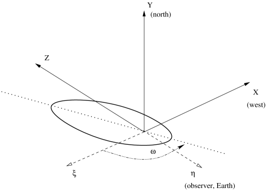
Figure 1: The geometry of the orbit of the transiting planet. The plane of the sky is defined by the $X+$ (west) and $Y+$ (north) axes while the $Z+$ axis points away from the Earth. The orbital plane is defined by the axes $\xi+$ and $\eta+$, where $\xi+$ is anti-parallel with $X+$ axis, $\eta+$ is in the plane of $(Y+,Z+)$ and the angle between $Y+$ and $\eta+$ is the inclination, nearly $90^{\circ}$. The major axis of the orbit is marked by the dotted line.

Now let us denote the mean longitude of the planet at the instance of the transit by $\lambda$. For a circular orbit, $\lambda=\varphi_{0}$. From its standard definition in celestial mechanics, it is straightforward to derive the mean longitude for arbitrary eccentricities (see Appendix A). The result is

$$\lambda \equiv \lambda(\varphi_{0},k,h)\equiv\lambda(\varphi_{0},e\cos\omega,e\sin\omega)=$$ (1)

$$= \mathop{\mathrm{arg}}\nolimits\left(k+\cos\varphi_{0}+\frac{he_{\perp}}{2-\ell},h+\sin\varphi_{0}-\frac{ke_{\perp}}{2-\ell}\right)-$$

$$-\frac{e_{\perp}(1-\ell)}{1+e_{\parallel}},$$

where $e_{\parallel}=k\cos\varphi_{0}+h\sin\varphi_{0}$, $e_{\perp}=k\sin\varphi_{0}-h\cos\varphi_{0}$ are the components of the eccentricity vector relative to the line-of-sight, $\ell=1-\sqrt{1-e^{2}}$ is the oblateness of the orbit, and $\mathop{\mathrm{arg}}\nolimits(x,y)=\arctan(y/x)$ if $x\geq 0$ and $\pi+\arctan(y/x)$ otherwise. Plugging in the observed values of $e$ and $\omega$, equation (1) provides a simple way of calculating the mean longitude of the orbit for an arbitrary transit observation. Note that this formalism omits the direct usage of the mean anomaly, true anomaly and eccentric anomaly which have no meanings for $e\to 0$. All of our derived formulae are based on the well–behaved parameters $\lambda$, $k$, and $h$, and therefore are valid for arbitrary eccentricities.

In the following subsections, we derive the expressions describing TTVs and TDVs, discuss the corresponding observational implications and estimate the precision of periastron precession observations.

Table 1: Basic data of the four known eccentric transiting exoplanetary systems: the mass ($M_{\star}$) of the parent star, period ($P$, in days), eccentricity ($e$) and the argument of pericenter ($\omega$), the half-duration of a transit event ($H$, in days) and the impact parameter ($b$). In the last two columns, we provide the calculated values of the secular period caused by the GR periastron precession, and the minimum mass – semimajor axis ratio for a hypothetical exterior perturber at $a_{2}\gtrsim 3a$ that would lead to the same magnitude of periastron precession.

. System $M_{\star}/M_{\odot}$ $P$ (d) $e$ $\omega$ (degrees) $H$ (d) $b$ $P_{\rm sec}$ (years) $\frac{m_{2}/M_{\oplus}}{(a_{2}/3a)^{3}}$ HD 147506b $1.298\pm 0.07$ $5.63341$ $0.520\pm 0.010$ $179.3\pm 3.6$ $0.083$ $0$ $19790\pm 740$ $12.2$ XO-3b $1.41\pm 0.08$ $3.19154$ $0.260\pm 0.017$ $344.6\pm 6.6$ $0.050$ $0.8$ $9280\pm 410$ $15.9$ GJ 436b $0.452\pm 0.013$ $2.64385$ $0.150\pm 0.012$ $351.0\pm 1.2$ $0.065$ $0.85\pm 0.02$ $15180\pm 400$ $2.6$ HD 17156b $1.2\pm 0.1$ $21.21725$ $0.6717\pm 0.0027$ $121.23\pm 0.40$ $0.098$ $0.50\pm 0.12$ $143000\pm 7900$ $5.9$

2.1 Modulation of the transit period

The period between successive transits $P_{\mathrm{\rm obs}}$ is modified by a possible slow precession of the orbital elements. These modulations are referred to as transit timing variations (TTVs). We derive the modulation of $P_{\rm obs}$ due to periastron precession in two steps. First we demonstrate that the change in the period between successive transits is simply related to the change in the mean longitude $\Delta\lambda$. Then relating the mean longitude shift to the periastron precession rate we derive the expected TTV rate.

Let $P_{0}$ be the orbital period, $n=2\pi/P_{0}$ be the mean angular velocity. The mean longitude of the planet increases steadily in time, $\lambda=nt+\lambda_{0}$. The variation in the mean longitude at the transit center would result in a variation in the transit cadence. During a transit at time $t_{1}$, the mean longitude is $\lambda_{\rm tr}(t_{1})=nt_{1}+\lambda_{0}$, and after an observed revolution, at the instance $t_{2}=t_{1}+P_{\mathrm{\rm obs}}$ it is $\lambda_{\rm tr}(t_{2})+2\pi=nt_{2}+\lambda_{0}$. Therefore the observed period between transits is

$$P_{\mathrm{\rm obs}}=\frac{2\pi+\Delta\lambda}{n}=P_{0}\left(1+\frac{\Delta\lambda}{2\pi}\right)$$ (2)

where $\Delta\lambda=\lambda_{\rm tr}(t_{2})-\lambda_{\rm tr}(t_{1})$.

In the following we assume that the shift in the mean longitude is caused by the perihelion shift $\Delta\omega=P_{0}\dot{\omega}$ per period, (i.e. we assume a constant eccentricity), then from the chain rule

$$\Delta\lambda=\frac{\partial\lambda}{\partial\omega}\Delta\omega=\frac{\partial\lambda}{\partial k}\frac{\partial k}{\partial\omega}\Delta\omega+\frac{\partial\lambda}{\partial h}\frac{\partial h}{\partial\omega}\Delta\omega.$$ (3)

Here $\partial k/\partial\omega=-e\sin\omega$ and $\partial h/\partial\omega=e\cos\omega$, from definition (see above), and the partial derivatives $\partial\lambda/\partial k$ and $\partial\lambda/\partial h$ can be found from equation (1) and are given explicitly in the Appendix (47–48). At transit, we get

$$\frac{\partial\lambda}{\partial\omega}=\frac{e^{2}}{1+\sqrt{1-e^{2}}}+\sqrt{1-e^{2}}\frac{e^{2}+(2+e\sin\omega)e\sin\omega}{(1+e\sin\omega)^{2}}.$$ (4)

Combining equations (2)-(4) and defining the secular period of the periastron precession as $P_{\rm sec}=(2\pi)/\dot{\omega}$, we get

$$P_{\mathrm{\rm obs}}=P_{0}+\frac{P_{0}^{2}}{2\pi}\frac{\partial\lambda}{\partial\omega}\dot{\omega}=P_{0}+\frac{\partial\lambda}{\partial\omega}\frac{P_{0}^{2}}{P_{\rm sec}}.$$ (5)

Since $\partial\lambda/\partial\omega$ itself is not constant due to periastron precession, the observed period between transits slowly changes. Differentiating equation (5) with respect to time, we get

$$\dot{P}_{\rm obs}=2\pi\frac{\partial^{2}\lambda}{\partial\omega^{2}}\frac{P_{0}^{2}}{P_{\rm sec}^{2}}=\frac{4\pi(1-e^{2})^{3/2}e\cos\omega}{(1+e\sin\omega)^{3}}\frac{P_{0}^{2}}{P_{\rm sec}^{2}},$$ (6)

since the partial derivative of equation (4) with respect to $\omega$ is

$$\frac{\partial^{2}\lambda}{\partial\omega^{2}}=\frac{2(1-e^{2})^{3/2}e\cos\omega}{(1+e\sin\omega)^{3}}.$$ (7)

Note that this equation clearly shows that the small eccentricity approximation $\partial^{2}\lambda/\partial\omega^{2}\approx e\cos\omega$ (e.g. used by Miralda-Escude, 2002; Heyl & Gladman, 2007) is very imprecise for moderate to large eccentricites. Depending on the actual value of $\omega$, equation (7) can result even $6-8$ times smaller or larger values for $\partial^{2}\lambda/\partial\omega^{2}$ as its first order approximation for eccentricities $0.5-0.7$.

We have to mention here that the observed period and therefore the individual transit timings are also affected by the light time effect (LTE). Since the precession of an elliptical orbit causes the distance between the host star and the planet at the transit instances to vary, the light time delay will change for transit event to transit event. The magnitude of this effect can be derived as follows. The distance between the star and the planet at transit time (i.e. when $\lambda=\varphi_{0}=\pi/2$) is

$$r=\frac{a(1-e^{2})}{1+e\cos v}=\frac{a(1-e^{2})}{1+e\cos(\varphi_{0}-\omega)}=\frac{a(1-e^{2})}{1+e\sin\omega}.$$ (8)

This difference in the distance implies an additional $-r(1-\mu)/c$ time shift, respective to the barycentric reference frame of the star–planet system. Here, $\mu=M_{\rm p}/(M_{\rm p}+M_{\star})\ll 1$ is the mass parameter, $a$ is the semimajor axis of the orbit and $c$ is the speed of light. Therefore, the correction in the observed period is

$$P^{\rm+LTE}_{\mathrm{\rm obs}} = P_{\mathrm{\rm obs}}-\frac{a}{c}(1-e^{2})\frac{\partial(1+e\sin\omega)^{-1}}{\partial\omega}P_{0}\dot{\omega}=$$ (9)

$$= P_{\mathrm{\rm obs}}+2\pi\frac{a}{c}\frac{(1-e^{2})e\cos\omega}{(1+e\sin\omega)^{2}}\frac{P_{0}}{P_{\rm sec}},$$

where we neglected the barycentric correction. Thus, the variation in this period (corrected for LTE) due to the variation in $\omega$ is

$$\dot{P}^{\rm+LTE}_{\mathrm{\rm obs}}=\dot{P}_{\mathrm{\rm obs}}-4\pi^{2}(1-e^{2})\frac{e(e+e\cos^{2}\omega+\sin\omega)}{(1+e\sin\omega)^{3}}\frac{a}{c}\frac{P_{0}}{P_{\rm sec}^{2}}.$$ (10)

Comparing equation (6) and (10), and assuming that the motion of the planet is non-relativistic, $a/c\ll P_{0}$, we find that $|\dot{P}^{\rm+LTE}_{\mathrm{\rm obs}}-\dot{P}_{\mathrm{\rm obs}}|\ll|\dot{P}_{\mathrm{\rm obs}}|$. We conclude that the period variation due to the LTE is negligible compared to the period variation caused by the changing geometry.

In summary, equations (5)-(6), along with equation (4), give the modulation of the actual observable period between transit events. These results are valid for arbitrary eccentricities and are independent of the physical mechanism causing the secular precession of the periastron. We calculate the secular precession period caused by general relativity (see e.g., Wald, 1984) using

$$P_{\rm sec}=\frac{c^{2}(1-e^{2})}{3(2\pi GM_{\star})^{2/3}}P_{0}^{5/3},$$ (11)

where $M_{\star}$ is the mass of the parent star, $G$ is Newton’s gravitational constant. This secular period is of order $10^{4}$–$10^{5}\,$years for the known ETEP systems (see Table 1 and Section 3 for more details). We note that if other planets are also present in these systems, they might also cause additional periastron precession of a larger magnitude. The Yarkovski-effect (Fabrycky, 2008) and the tidal circularization (see Johns-Krull et al., 2007, and the references therein) lead to negligible modifications for our purposes, as these effects are relevant on timescales exceeding $0.1\,$Gyr for these systems. In the following, we compare the precession measurement sensitivities with the general relativistic rate $P_{\rm sec}$ given by equation (11).

2.2 Modulation of the transit duration

Here we investigate how the periastron precession affects the duration of a transit. Let us denote the half duration of the transit by $H=T_{\rm D}/2$, which we define as half the time between the instances when the center of the planetary disk intersects the limb of the star, i.e. between the center of the ingress and egress. Note that this is not the time between the first and last contact. This is important because the instances of the center of the ingress and egress can be measured more accurately than their beginning or end. Since we are interested in estimating the variations of the duration of the transit to leading order, we perform a first-order calculation, i.e. assuming a constant apparent tangential velocity for the planet and neglecting the changes in the impact parameter due to the elliptical orbit and/or the curvature of the projection of the orbit due to the inclination. From Kepler’s Second Law and equation (8), one can calculate the tangential distance $\Delta x$ traveled by the planet during time $H$,

$$\Delta x=v_{\rm tan}H=an\frac{1+e\sin\omega}{\sqrt{1-e^{2}}}H$$ (12)

(see Appendix B for the derivation of $v_{\rm tan}$). This can be related to the impact parameter $b$ and the radius of the star $R_{\star}$ for the geometry of the transit as

$$\frac{\Delta x}{R_{\star}}=\sqrt{1-b^{2}}.$$ (13)

Thus, to leading order,

$$H=\frac{P_{0}}{2\pi}\left\{\frac{R_{\star}}{a}\frac{\sqrt{1-e^{2}}}{1+e\sin\omega}\sqrt{1-b^{2}}+\mathcal{O}\left[\left(\frac{R_{\star}}{a}\right)^{3}\right]\right\}.$$ (14)

Note that equation (14) depends on $\omega$ through the $(1+e\sin\omega)^{-1}$ term and also implicitly through $b$,

$$b=\frac{r\cos i}{R_{\star}}=\frac{a}{R_{\star}}\frac{1-e^{2}}{1+e\sin\omega}\cos i.$$ (15)

The variation in $H$ caused by the variation in the periastron can be found from equation (14) and (15),

$$\frac{\partial H}{\partial\omega}=\frac{e\cos\omega}{1+e\sin\omega}H\frac{1-2b^{2}}{1-b^{2}}.$$ (16)

Note that equation reflects the qualitative expections implied by Kepler’s Second Law. Namely, if an eccentric orbit advances, the distance between the planet and the star will change. If this distance decreases, the impact parameter will also decrease (resulting a longer transit duration) but due to Kepler’s Second Law, the apparent tangential velocity of the transiting object will increase (resulting a shorter transit duration). Therefore at a certain value of the inclination and/or the impact parameter, the two effects cancel each other yielding no TDV effect. Equation 16 clearly shows that it occurs when the impact parameter is $b=1/\sqrt{2}\approx 0.707$. The long-term variation in the duration of the transit is then

$$\dot{H}=\frac{\partial H}{\partial\omega}\dot{\omega}=\frac{\sqrt{1-e^{2}}e\cos\omega}{(1+e\sin\omega)^{2}}\frac{1-2b^{2}}{\sqrt{1-b^{2}}}\frac{R_{\star}}{a}\frac{P_{0}}{P_{\rm sec}}$$ (17)

Comparing equation (6) and equation (17) the TDV effect relates to the TTV effect as

$$\frac{\dot{H}}{\dot{P}_{\rm obs}}=\frac{1+e\sin\omega}{6\pi}\frac{1-2b^{2}}{\sqrt{1-b^{2}}}\frac{R_{\star}}{R_{\rm Sch}}$$ (18)

where $R_{\rm Sch}=2GM/c^{2}$ is the Schwarzschild radius of the star. As an example, note that $R_{\star}/R_{\rm Sch}=2.5\times 10^{5}$ for the Sun. Therefore, equation (18) shows that the TDV effect is always much larger than the TTV effect. In particular, the ratio is larger for increasing $b$. In the limit $b\to 1$ equation (17) breaks down because the periastron precession shifts the orbit out of the transiting region.

2.3 Observational implications

Now, using the results for the TDV and TTV effects, equation (6) and (17), we can estimate how these timing and transit duration variations might be observed on long timescales. In the following we discuss these observational implications.

2.3.1 Transit Timing Variations

Equation (6) shows that the observed period between successive transits increases or decreases at a practically constant rate during the observations, $\dot{P}_{\mathrm{\rm obs}}$. The time of the $m$th transit from an arbitrary epoch $T_{0}$ can be found from adding up the contributions of the observed $m$ number of periods

$$T_{m} = T_{0}+P_{\mathrm{\rm obs}}m+Dm^{2},$$ (19)

where $P_{\mathrm{\rm obs}}\approx P_{0}$ denotes the time of the first observed orbit, $D$ is the transit timing variation factor,

$$D=\frac{P_{0}\dot{P}_{\mathrm{\rm obs}}}{2}=2\pi G_{\rm TV}(e,\omega)P_{0}\left(\frac{P_{0}}{P_{\rm sec}}\right)^{2},$$ (20)

where we have introduced the geometrical factor

$$G_{\rm TV}(e,\omega)=(1-e^{2})^{3/2}\frac{e\cos\omega}{(1+e\sin\omega)^{3}}.$$ (21)

The chance of detecting the periastron precession increases with the geometrical factor $G_{\rm TV}(e,\omega)$ which is related to the alignment of the orbital ellipse with the line of sight. The optimal value for detecting the precession is $\omega=0$ or $\pi$ for small eccentricities, i.e. the semimajor axis should be perpendicular to the line of sight. For arbitrary eccentricities, the optimal value for $\omega$ for the TTV observation is

$$\omega^{\rm best}_{\rm TV}=\frac{3}{2}\pi\pm\arccos\left(\frac{6e}{1+\sqrt{1+24e^{2}}}\right).$$ (22)

which approaches $0^{\circ}$ and $180^{\circ}$ for small eccentricities as expected, and $270^{\circ}$ for large eccentricities. In case of $e=0.5$, $\omega_{\rm extr}=\{235.4^{\circ},304.6^{\circ}\}$. The least favorable value for $\omega$ occurs when $G_{\rm TV}(e,\omega)=0$, i.e. at $\omega^{\rm worst}_{\rm TV}=\{90^{\circ},270^{\circ}\}$,.

2.3.2 Transit Duration Variations

Now let us turn to the TDV effect. The observed duration of the $m$th transit can be calculated in the same way, namely

$$H_{m}=H_{0}+Fm,$$ (23)

where $F$ is the shift in the transit duration per orbit. This factor is

$$F=P_{0}\dot{H}=2\pi G_{\rm DV}(e,\omega,b)H\frac{P_{0}}{P_{\rm sec}},$$ (24)

and

$$G_{\rm DV}(e,\omega,b)=\frac{1-2b^{2}}{1-b^{2}}\frac{e\cos\omega}{1+e\sin\omega}.$$ (25)

The optimal orientation $\omega^{\rm best}_{\rm DV}$ for detecting the TDV effect for fixed $e$, $b$, and $P_{0}$ can be found by maximizing $HG_{\rm DV}(e,\omega,b)$. The result is

$$\omega^{\rm best}_{\rm DV}=\frac{3}{2}\pi\pm\arccos\left(\frac{4e}{1+\sqrt{1+8e^{2}}}\right).$$ (26)

and the worst orientation is at $\omega^{\rm worst}_{\rm DV}=\{90^{\circ},270^{\circ}\}$, just like for the TTV case. Comparing $\omega^{\rm best}_{\rm TV}$ and $\omega^{\rm best}_{\rm DV}$ it is clear that the most favorable orientation in terms of the two effects are similar, hence the chance of detecting the periastron motion through transit timing variations or transit duration variations is correlated. Both effects go away if the eccentricity is oriented parallel to the line of sight. We also note that for moderate values of $e$ and small impact parameters, $|G_{\rm TV}|\approx|G_{\rm DV}|$ which also implies that the most favorable geometry for detecting either TTVs or TDVs is similar.

2.4 Error analysis

Next we estimate the parameter measurement precision of the TTV and TDV effects for future observations. We consider the repeated observation of a particular transiting system over a total timespan $T_{\rm tot}$, measuring the transit timing $T_{m}$ and duration $H_{m}$ for each transit with respective errors $\sigma(T)$ and $\sigma(H)$. (We discuss the specific values of $\sigma(T)$ and $\sigma(H)$ for transit observations in Section 3.1). For simplicity, let us assume that these measurements are equidistant and in total $N$ independent transits are observed, i.e. the $m$th transit is observed if $m=0,d,\dots,(N-1)d$, where $d=T_{\rm tot}/(NP_{0})$.

2.4.1 Transit Timing Variations

Using equation (19), we can fit a second-order polynomial to these observations with unknown coefficients $T_{0}$, $P_{\rm obs}$ and $D$ by minimizing the merit function

$$\chi^{2}_{\rm TV}=\sum\limits_{m=0,d,\dots,(N-1)d}\left[\frac{T_{m}-(T_{0}+P_{\rm obs}m+Dm^{2})}{\sigma(T)}\right]^{2}.$$ (27)

The minimization of the above function results in a linear set of equations in the parameters $p_{i}=\{T_{0},P_{\rm obs},D\}$. Assuming Gaussian errors, the parameter estimation covariance matrix can be found from the Fisher matrix method (Finn, 1992):

$$\left<\delta p_{i}\delta p_{j}\right>=(\mathcal{F}^{-1})_{ij}$$ (28)

Here $\mathcal{F}$ is the Fisher matrix defined as

$$\mathcal{F}_{ij}=\sum\limits_{m=0,d,\dots,(N-1)d}\frac{1}{\sigma^{2}(T)}\frac{\partial T^{\rm fid}_{m}}{\partial p_{i}}\frac{\partial T^{\rm fid}_{m}}{\partial p_{j}}$$ (29)

where $T^{\rm fid}_{m}$ is the fiducial value of $T_{m}$ given by equation (19). The marginalized expected squared parameter estimation error is given by the diagonal elements of the covariance error matrix $\sigma^{2}(p_{i})=(\mathcal{F}^{-1})_{ii}$. In particular, the resulting uncertainty of $D$ becomes

$$\sigma(D) = \frac{\sqrt{180}\,\sigma(T)}{d^{2}\sqrt{N(N^{2}-1)(N^{2}-4)}}$$ (30)

$$\approx \sqrt{180}\left(\frac{P_{0}}{T_{\rm tot}}\right)^{2}\left(1+\frac{5}{2N^{2}}\right)\frac{\sigma(T)}{\sqrt{N}}.$$

Here, the first equality is valid for arbitrary $N$, while the second is its first order approximation for large $N$. The leading order approximation is verified against Press et al. (1992).

2.4.2 Transit Duration Variations

We can repeat the same calculations as above for the observation of the half transit duration $H_{m}$ to measure the variation factor $F$. The merit function in this case

$$\chi^{2}_{\rm DV}=\sum\limits_{m=0,d,\dots,(N-1)d}\left[\frac{H_{m}-(H_{0}+Fm)}{\sigma(H)}\right]^{2},$$ (31)

has to be minimized for the same set of observations. This minimization again leads to a linear set of equations in the parameters $H_{0}$ and $F$. The Fisher matrix method in this case gives the uncertainty in $F$ as

$$\sigma(F) = \frac{\sqrt{12}\sigma(H)}{d\sqrt{N(N^{2}-1)}}\approx$$ (32)

$$\approx \sqrt{12}\frac{P_{0}}{T_{\rm tot}}\left(1+\frac{1}{2N^{2}}\right)\frac{\sigma(H)}{\sqrt{N}}.$$

Figure 2: The significance of detecting the GR periastron precession $|F_{0}|/\sigma_{0}(F)$ through the TDV effect as a function of orbital period and eccentricity. The transit duration is assumed to be measured for $4$ years each with a $5$ sec error, for a Sun-like star on a non-inclined orbit. Increasing the mass or radius of the star, or the impact parameter increases the detection significance (see text).

Figure 2 shows the detection significance of the TDV measurement $|F|/\sigma(F)$, if the precession rate in $F$ is given by the general relativistic formula, equation (24). Here each transit is assumed to be measured (i.e. $d=1$) with a precision $\sigma(H)=5$ sec for a total observation time of $T_{\rm tot}=4$ years. These assumptions are realistic for the future Kepler mission (see § 3.1 below). Other parameters are $M_{\star}=M_{\odot}$, $R_{\star}=R_{\odot}$, $b=0$, and we averaged over the possible orientations of $\omega$. For other parameters,

$$\frac{|F|/\sigma(F)}{|F_{0}|/\sigma(F_{0})} = \frac{1}{d}\frac{1}{\sqrt{1-b^{2}}}\left(\frac{R_{\star}}{R_{\odot}}\right)\left(\frac{M_{\star}}{M_{\odot}}\right)^{1/3}\cdot$$ (33)

$$\cdot\left(\frac{\sigma(H)}{5\,{\rm sec}}\right)^{-1}\left(\frac{T_{\rm tot}}{4\,{\rm yr}}\right)^{3/2},$$

implying that the detection significance can be even better.

Figure 2 clearly shows that the chances of detecting the precession effects through the TDV effect is encouraging. The detection significance of the general relativistic precession of a transiting exoplanet with eccentricity $e\gtrsim 0.2$ and period $P\lesssim 5$ days, is typically over the $1$-$\sigma$ level. Generally, equation (30) and equation (32) can be used directly to check what kind of observations are required to detect the precession of the periastron through the TTV or TDV methods, respectively.

3 The case of XO-3b, HD 147506b, GJ436b and HD 17156b

As of this writing, four TEPs are known with a non-zero eccentricity within $3$-$\sigma$, namely XO-3b (Johns-Krull et al., 2007), HD 147506b (Bakos et al., 2007), GJ 436bb (Butler et al., 2004; Gillon et al., 2007), and HD 17156bb (Fischer et al., 2007; Barbieri et al., 2007). The planet TrES-1 (Alonso et al., 2004) has also been reported as an object with non-zero eccentricity, however, it is zero within $2$-$\sigma$ thus we omit from our analysis. We note here that recently both GJ 436 and HD 17156 have been suggested to have another planetary companions (see Ribas et al., 2008; Short et al., 2008). The secular period of the periastron motion are determined by the mass of the star $M_{\star}$, the orbital period $P_{0}$, and the eccentricity $e$, while the timing variation constant $D$ is also affected by the actual argument of pericenter, $\omega$. The transit duration variation factor $F$ is affected indirectly by the geometrical ratio $a/R_{\star}$ and directly by the impact parameter $b$. These parameters are summarized in the first seven columns of Table 1 for these four ETEP systems. The derived GR periastron precession period, $P_{\rm sec}$ can be found in the 8th column of the table.

In addition to the inevitable periastron precession caused by GR, there might be other sources of perturbations causing periastron precession. The last column gives the minimum mass to semimajor axis ratio of a hypothetical exterior perturber (e.g. a planet or an asteroid belt), in Earth mass units, which causes the same periastron presession rate as that caused by the general relativity. This estimate based on Price & Rush (1979), and is valid for $a_{2}\gtrsim 3a$ and for non-resonant cases. Note that the minimum mass of the perturber scales with the third power of the semimajor axis ratio to cause a comparable precession rate as GR. The numbers show that the precession caused by additional planets in the system, if present, can easily cause a larger precession rate than GR. In case of orbital resonances with exterior planets, the precession rate can be even larger (Holman & Murray, 2005; Agol et al., 2005). To be conservative, we examine whether the precession rate can be measured to a precision better than that corresponding to GR.

To obtain a high significance, $k$-$\sigma$ detection of the periastron precession using transit timing variations, we need $k\sigma(D)\approx|D|$. Using equation (30), the total number of transits necessary to measure $D$ with this precision is

$$N_{\rm TV}=180\left[\frac{\sigma(T)}{k|D|}\right]^{2}\left(\frac{P_{0}}{T_{\rm tot}}\right)^{4}.$$ (34)

Thus, the number of such required transit observations is extremely sensitive to the orbital period $P_{0}$ and the observation timespan. Table 2 gives the corresponding values of the transit timing variation factors for the known ETEP systems and this number of observations, assuming a $T_{\rm tot}=20$ year long observational timespan, timing precision of $\sigma(T)=2~{}{\rm sec}$ and $3$-$\sigma$ sensitivity of the GR periastron precession level. The table shows the recently discovered XO-3b system is a promising candidate to detect the GR periastron precession through the TTV effect, while the other ETEP systems require unrealistically many observations. We note that if other perturbing planets are present in these systems and lead to a precession rate that is larger by a factor of 10 than the GR precession rate, then the number of detections (during the same $T_{\rm tot}$ timespan) is lower by a factor of 100. It is interesting that the best candidate (by far) is XO-3b even though its eccentricity is not as large as that of HD 147506b or HD 17156b.

Table 2: Transit timing variation factor ($D$, in seconds) and the number of transits ($N_{20\,{\rm y},3-\sigma,2\,{\rm sec}}$) what should be detected almost uniformly in a 20 year long timespan, each with an error of $2$ second to confirm the precession within $3$-$\sigma$.

System	$D$ (seconds)	$N_{20\,{\rm y},~{}3-\sigma,~{}2\,{\rm sec}}$
HD 147506b	$-(5.9\pm 0.7)\cdot 10^{-7}$	$6600$
XO-3b	$+(4.3\pm 0.6)\cdot 10^{-7}$	$1280$
GJ 436b	$+(5.0\pm 0.5)\cdot 10^{-8}$	$44160$
HD 17156b	$-(6.9\pm 0.8)\cdot 10^{-8}$	$97\cdot 10^{6}$

Table 3: Transit duration variation factor ($F$, in seconds) and the number of transits ($N_{2\,{\rm y},~{}3-\sigma,~{}2\,{\rm sec}}$) what should be detected almost uniformly in a 4 year long timespan, each with an error of $2$ sec to confirm the precession within $3$-$\sigma$.

System	$F$ (seconds)	$N_{4\,{\rm y},~{}3-\sigma,~{}2\,{\rm sec}}$
HD 147506b	$-(1.8\pm 0.3)\cdot 10^{-2}$	$20$
XO-3b	$-(5.4\pm 0.6)\cdot 10^{-3}$	$70$
GJ 436b	$-(4.1\pm 0.5)\cdot 10^{-3}$	$85$
HD 17156b	$-(3.2\pm 0.2)\cdot 10^{-3}$	$8970$

Let us now turn to the observational constraints for the detection of transit duration variations. Using equation (32), the total number of required observations within $T_{\rm tot}$ is

$$N_{\rm DV}=12\left[\frac{\sigma(H)}{k|F|}\right]^{2}\left(\frac{P_{0}}{T_{\rm tot}}\right)^{2}.$$ (35)

Note that $N_{\rm DV}$ is not as sensitive to the $P_{0}/T_{\rm tot}$ ratio as $N_{\rm TV}$, and implies that a smaller number of observations is typically necessary.

In Table 3 we present the values of the transit duration variation factor, $F$, and the number of required observations to reach the same $3$-$\sigma$ confidence for detecting the GR periastron precession. Here we assumed a shorter observation timespan, $T_{\rm tot}=4$ year (i.e. shorter compared to the 20 year long timespan necessary for the detection of the TTV effect), the same timing precision of $\sigma(H)=2~{}{\rm sec}$ and the same level of detection, $3$-$\sigma$. The best known ETEP system for TDV detection is therefore HD 147506b, but the number of necessary observations is feasible for XO-3b and GJ 436b as well.

3.1 Photometric detection

The precision for measuring the transit timing and transit duration for a photometric observation can be estimated as follows. Since the time of the ingress ($T_{\rm I}$) and the time of the egress ($T_{\rm E}$) – i.e. when the center of the planet crosses the limb of the star inwards or outwards, respectively – defines both the time of the transit center and the half duration like

$$T = \frac{1}{2}(T_{\rm E}+T_{\rm I}),$$ (36)

$$H = \frac{1}{2}(T_{\rm E}-T_{\rm I}),$$ (37)

moreover $T_{\rm I}$ and $T_{\rm E}$ can be treated as uncorrelated variables, therefore the uncertainties of the transit time and half duration would be nearly the same, i.e. $\sigma(T)\approx\sigma(H)$. We have estimated these uncertainties for the four distinct planets using Monte-Carlo simulations by fitting transit light curves on mock data sets. We have used the observed planetary parameters as an input for these artificial light curves. The fit was performed assuming quadratic limb darkening (see Mandel & Agol, 2002) in the Sloan $z^{\prime}$ band. The mock light curves were sampled with $\Delta\tau_{1}=1\,{\rm sec}$ cadence and an additional Gaussian noise of $\sigma_{1}(m)=1\,{\rm mmag}$ was added. The resulting uncertainties, $\sigma_{1,1}(T)$ and $\sigma_{1,1}(H)$ for the four planets are presented in Table 4. Since the depth of the four transits are nearly the same (see the appropriate normalized radii, $p=R_{p}/R_{\star}$, all between $0.068\lesssim p\lesssim 0.085$), the uncertainties $\sigma_{1,1}(T)$ and $\sigma_{1,1}(H)$ are almost the same for the four cases. Using these normalized values, one can easily estimate the uncertainties for arbitrary sampling cadence $\Delta\tau$ and photometric precision $\sigma(m)$ using

$$\sigma(T) \approx \sigma_{1,1}(T)\frac{\sigma(m)}{1\,\rm mmag}\sqrt{\frac{\Delta\tau}{1\,\rm sec}},$$ (38)

$$\sigma(H) \approx \sigma_{1,1}(H)\frac{\sigma(m)}{1\,\rm mmag}\sqrt{\frac{\Delta\tau}{1\,\rm sec}}.$$ (39)

For comparison, note that the expected photometric precision of the Kepler space telescope (see Borucki et al., 2007) is $1\,{\rm mmag}$ for observing a light curve of a bright, $M_{v}=8.8$ star with a $1\,{\rm sec}$ sampling cadence. Since the star XO-3 has almost the same apparent magnitude, it is clear, the transit durations would be detected with an accuracy of $\sigma(H)\approx 5\,{\rm sec}$ if this star was in the field of Kepler. Therefore, equation (32) and Table 3 shows that the transit duration variations would be detectable for HD 147506(b) or XO-3(b)–like systems due to the GR periastron precession, within $3$-$\sigma$ confidence with a Kepler–type mission within approximately 3 or 4 years, respectively.

Table 4: Uncertainties of the transit time and transit duration measurements for the four known ETEPs, assuming Sloan $z^{\prime}$-band photometric data taken with a 1 sec cadence and 1 mmag photometric precision.

System	$\sigma_{1,1}(T)$ (sec)	$\sigma_{1,1}(H)$ (sec)
HD 147506b	5.3	4.8
XO-3b	6.9	4.7
GJ 436b	6.7	8.4
HD 17156b	5.4	6.1

4 Summary

The first four eccentric transiting exoplanetary systems have been discovered during 2007. The precession of an eccentric orbit causes variations both in the transit timings and transit durations. We estimated the significance of measuring the corresponding observable effects compared to the inevitable precession rate of general relativity. We applied these calculations to predict the significance of measuring the effect for the four known eccentric transiting planetary systems. Our calculations show that a space-borne telescope is adequate to detect the change in the transit durations to a high significance better than the GR periastron precession rate within a 3 – 4 year timespan (in a continuous observing mode). The same kind of instruments would need more than a decade to detect the corresponding transit time variations to this sensitivity even for the most optimistic known system.

The CoRoT mission has already found two transiting planets (see Barge et al., 2008; Alonso et al., 2008) and there are two known planets in the planned field-of-view of the Kepler mission (see O’Donovan et al., 2006; Pál et al., 2008). Our results suggest that if an eccentric transiting planet is found in the Kepler or CoRoT field, these missions will be able to measure the periastron precession rate to a very high significance within their mission lifetime or with the support of ground-based observations on a longer time scale. This will provide an independent test of the theory of general relativity and will also be useful for testing for the presence of other planets in these systems.

Appendix A Mean longitude at the transit instances

The derivation of equation (1) goes as follows. According to Kepler’s equation, $E-e\sin E=M=\lambda-\omega$, one can write $\lambda=\omega+E-e\sin E$. The only thing what is to be done is to calculate the eccentric anomaly $E$ for the instance when the orbiting body intersect the semi-line with the argument angle $\varphi_{0}$. The latter means that the true anomaly $v$ of the body is $v=\varphi_{0}-\omega$, by definition. The relation between the eccentric and true anomaly is

$$\tan\frac{E}{2}=\sqrt{\frac{1-e}{1+e}}\tan{\frac{v}{2}},$$ (40)

which is equivalent with

$$\cos E = \frac{e+\cos v}{1+e\cos v},$$ (41)

$$\sin E = \frac{\sqrt{1-e^{2}}\sin v}{1+e\cos v}.$$ (42)

Using the addition theorem, the sine and cosine of the angle $\omega+E$ can be written as:

$$\cos(\omega+E) = \cos\omega\frac{e+\cos(\varphi_{0}-\omega)}{1+e\cos(\varphi_{0}-\omega)}-$$ (43)

$$-\sin\omega\frac{\sqrt{1-e^{2}}\sin(\varphi_{0}-\omega)}{1+e\cos(\varphi_{0}-\omega)},$$

$$\sin(\omega+E) = \sin\omega\frac{e+\cos(\varphi_{0}-\omega)}{1+e\cos(\varphi_{0}-\omega)}+$$ (44)

$$+\cos\omega\frac{\sqrt{1-e^{2}}\sin(\varphi_{0}-\omega)}{1+e\cos(\varphi_{0}-\omega)}.$$

Thus, the mean longitude itself is going to be

$$\lambda = \omega+E-e\sin E=\mathop{\mathrm{arg}}\nolimits\left[\cos(\omega+E),\sin(\omega+E)\right]-$$ (45)

$$-e\frac{\sqrt{1-e^{2}}\sin v}{1+e\cos v}.$$

If both arguments of the above $\mathop{\mathrm{arg}}\nolimits[\cdot,\cdot]$ function is multiplied by the always positive common denominator $1+e\cos(\varphi_{0}-\omega)$, one gets after some simplification:

$$\omega+E = \mathop{\mathrm{arg}}\nolimits\left[k+\cos\varphi_{0}+\frac{h(k\sin\varphi_{0}-h\cos\varphi_{0})}{1+\sqrt{1-e^{2}}},\right.$$ (46)

$$\left.h+\sin\varphi_{0}-\frac{k(k\sin\varphi_{0}-h\cos\varphi_{0})}{1+\sqrt{1-e^{2}}}\right].$$

Putting all terms together and replacing the appropriate terms by $e_{\perp}=k\sin\varphi_{0}-h\cos\varphi_{0}$, $e_{\parallel}=k\cos\varphi_{0}+h\sin\varphi_{0}$ and $\ell=1-\sqrt{1-e^{2}}$, we get equation (1). The partial derivatives of equation (1) become

$$\frac{\partial\lambda}{\partial k} = -\frac{h}{2-\ell}-(1-\ell)\frac{h+(2+e_{\parallel})\sin\varphi_{0}}{(1+e_{\parallel})^{2}},$$ (47)

$$\frac{\partial\lambda}{\partial h} = +\frac{k}{2-\ell}+(1-\ell)\frac{k+(2+e_{\parallel})\cos\varphi_{0}}{(1+e_{\parallel})^{2}}.$$ (48)

Appendix B Tangential velocity and position at the transit

It is known from the theory of the two-body problem that the angular momentum of a body orbiting around a mass of $GM=\mu$ and having an orbit with the semimajor axis of $a$ and eccentricity $e$ is $C=\sqrt{\mu a(1-e^{2})}$. Since $C=rv_{\rm tan}$ for all points, the tangential velocity would be

$$v_{\rm tan}=\frac{C}{r}=\sqrt{\mu a(1-e^{2})}\frac{1+e\cos(\varphi_{0}-\omega)}{a(1-e^{2})}$$ (49)

Using Kepler’s Third Law, i.e. $\mu=n^{2}a^{3}$, the above equation can be reordered to

$$v_{\rm tan}=an\frac{1+e\cos(\varphi_{0}-\omega)}{\sqrt{1-e^{2}}}.$$ (50)

For $\varphi_{0}=\pi/2$, equation (50) becomes

$$v_{\rm tan}=an\frac{1+e\sin\omega}{\sqrt{1-e^{2}}}.$$ (51)

References

- Agol et al. (2005) Agol, E., Steffen, J., Sari, R., & Clarkson, W., 2005, MNRAS, 359, 567
- Alonso et al. (2004) Alonso, R. et al., 2004, ApJ, 613, 153
- Alonso et al. (2008) Alonso, R. et al., 2008, astro-ph:0803.3207
- Bakos et al. (2007) Bakos, G. Á. et al., 2007, ApJ, 670, 826
- Barbieri et al. (2007) Barbieri, M. et al., 2007, A&A, 476, 13
- Barge et al. (2008) Barge, P. et al., 2008, astro-ph:0803.3202
- Borucki et al. (2007) Borucki, W. J. et al., 2007, ASP Conf. Ser., 366, 309
- Brown et al. (2001) Brown, T. M. et al., 2001, ApJ, 552, 699
- Butler et al. (2004) Butler et al., 2004, ApJ, 617, 580
- Charbonneau et al. (2000) Charbonneau, D., Brown, T. M., Latham, D. W. & Major, M., 2000, ApJ, 529, 45
- Fischer et al. (2007) Fischer, D. A. et al., 2007, ApJ, 669, 1336
- Fabrycky (2008) Fabrycky, D., 2008, astro-ph:0803.1839
- Finn (1992) Finn, L. S., 1992, Phys. Rev. D, 46, 5236
- Ford & Holman (2007) Ford, E. B. & Holman, M. J., 2007, ApJ, 664, 51
- Gillon et al. (2007) Gillon, M. et al., 2007, A&A, 472, 13
- Heyl & Gladman (2007) Heyl, J. S. & Gladman, B. J., 2007, MNRAS, 377, 1511
- Holman & Murray (2005) Holman, M. J, & Murray, N. W., 2005, Science, 307, 1288
- Iorio (2006) Iorio, L., 2006, NewA, 11, 490
- Jordan & Bakos (2008) Jordan,A. & Bakos, G, 2008, ApJ, in press
- Johns-Krull et al. (2007) Johns-Krull, C .M. et al., 2007, astro-ph:0712.4283
- Mandel & Agol (2002) Mandel, K., Agol, E., 2002, ApJ, 580, 171
- Miller-Ricci et al. (2008) Miller-Ricci, E. et al., 2008, astro-ph:0802.0718
- Miralda-Escude (2002) Miralda-Escude, J., 2002, ApJ, 564, 1019
- Misner, Thorne, & Wheeler (1973) Misner, C. W., Thorne, K., & Wheeler, J. A., 1973, Gravitation, Second Edition, W. H. Freeman and Company, San Francisco
- O’Donovan et al. (2006) O’Donovan, F. T. et al., 2006, ApJ, 651, 61
- Pál et al. (2008) Pál, A. et al., 2008, astro-ph:0803.0746
- Press et al. (1992) Press, W. H., Teukolsky, S. A., Vetterling, W. T. & Flannery, B. P., 1992, Numerical Recipes in C: the art of scientific computing, Second Edition, Cambridge University Press
- Price & Rush (1979) Price, M. P., & Rush, W. E., 1979, Am. J. Phys., 47, 531
- Ribas et al. (2008) Ribas, I., Font-Ribera, A. & Beaulieu, J., 2008, ApJ, 677, 59
- Short et al. (2008) Short, D., Welsh, W. F., Orosz, J. A. & Windmiller G., 2008, astro-ph:0803.2935
- Simon et al. (2007) Simon, A., Szatmáry, K. & Szabó, Gy. M., 2007, A&A, 470, 727
- Steffen & Agol (2007) Steffen, J. H. & Agol, E., 2007, ASP Conf. Ser, 366, 158
- Wald (1984) Wald, R. M., 1984 General Relativity, The University of Chicago Press