PRIMORDIAL NON-GAUSSIANITY FROM MULTIPLE CURVATON DECAYS

We study a model where two scalar fields, that are subdominant during inflation, decay into radiation some time after inflation has ended but before primordial nucleosynthesis. Perturbations of these two curvaton fields can be responsible for the primordial curvature perturbation. We write down the full non-linear equations that relate the primordial perturbation to the curvaton perturbations on large scales, and solve them in a sudden-decay approximation. We calculate the power spectrum of the primordial perturbation, and finally go to second order to find the non-linearity parameter, $f_{\rm{NL}}$. Not surprisingly, we find large positive values of $f_{\rm{NL}}$ if the energy densities of the curvatons are sub-dominant when they decay, as in the single curvaton case. But we also find a novel effect, which can be present only in multi-curvaton models: $f_{\rm{NL}}$ becomes large even if the curvatons dominate the total energy density in the case when the inhomogeneous radiation produced by the first curvaton decay is diluted by the decay of a second nearly homogeneous curvaton. The minimum value $\min(f_{\rm{NL}})=-5/4$ which we find is the same as in the single-curvaton case. Using (non-)Gaussianity observations, Planck can be able to distinguish between single-field inflation and curvaton model. Hence it is important to derive theoretical predictions for curvaton model. From particle physics point of view it is more natural to assume multiple scalar fields (rather than just one “curvaton” in addition to inflaton). Our work updates the theoretical predictions of curvaton model to this case.

1 Introduction to curvaton model

Theories beyond the standard model often contain a large number of scalar fields in addition to the standard-model fields. In the very early universe it is natural to expect the initial values of these fields to be displaced from the minimum of their potential. If they are displaced by more than the Planck scale, then they can drive a period of inflation. Otherwise they will oscillate about the minimum of their potential once the Hubble rate, $H$, drops below their effective mass. An oscillating massive field has the equation of state (averaged over several oscillations) of a pressureless fluid. Thus the energy density of a weakly interacting massive field tends to grow relative to radiation in the early universe. Such fields must therefore decay before the primordial nucleosynthesis era to avoid spoiling the standard, successful hot big bang model. If the energy density of a late-decaying scalar is non-negligible when it decays, then any inhomogeneity in its energy density will be transfered to the primordial radiation.$\!{}^{{\bf?}}$ Therefore, the observed perturbations in the Universe can solely result from these inhomogeneities and the perturbations in the inflaton decay products (i.e., pre-existing radiation) can be negligible. This is the curvaton scenario for the origin of structure.$\!{}^{{\bf?}}$ We focus on this pure curvaton model.

2 Definitions: primordial perturbation, power spectrum, and $f_{\rm{NL}}$

The primordial density perturbation can be described in terms of the non-linearly perturbed expansion on uniform-density hypersurfaces $\!{}^{{\bf?}}$

$$\zeta(t,{\bf x})=\delta N(t,{\bf x})+\frac{1}{3}\int_{\bar{\rho}(t)}^{\rho(t,{\bf x})}\frac{d\tilde{\rho}}{\tilde{\rho}+\tilde{p}}\,,$$ (1)

where $N=\int Hdt$ is the integrated local expansion, $\tilde{\rho}$ the local density and $\tilde{p}$ the local pressure, and $\bar{\rho}$ is the homogeneous density in the background model. We will expand the curvature perturbation at each order $(n)$ as $\zeta(t,{\bf x})=\sum_{n=1}^{\infty}\frac{1}{n!}\zeta_{(n)}(t,{\bf x})\,,$ where we assume that the first-order perturbation, $\zeta_{(1)}$, is Gaussian as it is proportional to the initial Gaussian field perturbations. Higher-order terms describe the non-Gaussianity of the full non-linear $\zeta$.

Working in terms of the Fourier transform of $\zeta$, we define the primordial power spectrum as $\langle\zeta({\bf k_{1}})\zeta({\bf k_{2}})\rangle=(2\pi)^{3}P_{\zeta}(k_{1})\delta^{3}({\bf k_{1}}+{\bf k_{2}})\,.$ The average power per logarithmic interval in Fourier space is given by ${\cal P}_{\zeta}(k)=\frac{4\pi k^{3}}{(2\pi)^{3}}P_{\zeta}(k)\,,$ and is roughly independent of wavenumber $k$. The primordial bispectrum is given by $\langle\zeta({\bf k_{1}})\zeta({\bf k_{2}})\zeta({\bf k_{3}})\rangle=(2\pi)^{3}B(k_{1},k_{2},k_{3})\delta^{3}({\bf k_{1}}+{\bf k_{2}}+{\bf k_{3}})\,.$ The amplitude of the bispectrum relative to the power spectrum is commonly parameterized in terms of the non-linearity parameter, $f_{\rm{NL}}$, defined such that $B(k_{1},k_{2},k_{3})\!\!=\!\!(6/5)f_{\rm{NL}}\left[P(k_{1})P(k_{2})+2\,{\rm perms}\right]\,.$

As an example we will consider the primordial curvature perturbation produced by the decay of two scalar fields $a$ and $b$. Without loss of generality, we assume that the curvaton $a$ decays first when $H=\Gamma_{a}$ followed by the decay of the curvaton $b$ when $H=\Gamma_{b}$, where $\Gamma_{b}<\Gamma_{a}$.

During inflation the curvatons acquire an almost scale-invariant spectrum of perturbations on super-Hubble scales, ${\cal P}_{\delta a_{\ast}}={\cal P}_{\delta b_{\ast}}=H_{\ast}^{2}/(2\pi)^{2},$ where $H_{\ast}$ is the Hubble rate at Hubble exit. We assume that the field perturbations at Hubble exit have Gaussian and independent distributions, consistent with weakly-coupled isocurvature fluctuations of light scalar fields. When the Hubble rate drops below the mass of each curvaton field, the field begins to oscillate. The local value of each curvaton can evolve between Hubble-exit during inflation and the beginning of the field oscillations. We parameterize this evolution by functions $g_{a}$ and $g_{b}$, but we assume the two fields remain decoupled so that their perturbations remain uncorrelated. Thus at the beginning of curvaton oscillations, the curvaton fields have values $a_{\rm osc}=g_{a}(a_{\ast})$ and $b_{\rm osc}=g_{b}(b_{\ast})\,.$

We can define non-linear perturbation $\zeta_{a}$ and $\zeta_{b}$ for each curvaton analogous to the total perturbation (1). They become constant on scales larger than the Hubble scale once each curvaton starts oscillating, and while we can neglect energy transfer to the radiation, $\Gamma_{a}<H$. We find that the power spectra of $\zeta_{a}$ and $\zeta_{b}$ when the curvatons start to oscillate are related by $P_{\zeta_{b}}=\beta^{2}P_{\zeta_{a}}\,,$ where $\beta=\frac{g^{\prime}_{b}/g_{b}}{g^{\prime}_{a}/g_{a}}$ with $g^{\prime}_{b}\equiv\partial g_{b}/\partial b_{\ast}$ and similar for $g^{\prime}_{a}$. In this talk, we assume linear evolution between Hubble exit and the beginning of curvaton oscillations, so that $\beta$ reduces to the ratio of the background curvaton field values at Hubble exit, $\beta=a_{\ast}/b_{\ast}\,.$

3 Full non-linear equations

We will estimate the primordial density perturbation produced by the decay of two curvaton fields some time after inflation has ended using the sudden-decay approximation, generalizing the non-linear analysis of Ref. $\!{}^{{\bf?}}$ to the case of two curvatons. Before the decays we have three non-interacting fluids with barotropic equations of state and hence three curvature perturbations (1) which are constant on large scales

$$\textstyle\zeta_{\gamma}=\delta N+\frac{1}{4}\ln\left(\frac{\rho_{\gamma}}{\bar{\rho}_{\gamma}}\right)\,,\quad\quad\zeta_{a}=\delta N+\frac{1}{3}\ln\left(\frac{\rho_{a}}{\bar{\rho}_{a}}\right)\,,\quad\quad\zeta_{b}=\delta N+\frac{1}{3}\ln\left(\frac{\rho_{b}}{\bar{\rho}_{b}}\right)\,.$$ (2)

On the spatial hypersurface where $H=\Gamma_{a}$, there is an abrupt jump in the overall equation of state due to the sudden decay of the first curvaton into radiation, but the total energy density is continuous

$$\rho_{\gamma_{1}1}+\rho_{b1}=\rho_{\gamma_{0}1}+\rho_{a1}+\rho_{b1}\,.$$ (3)

Here $\rho_{\gamma_{1}1}$ is the radiation energy density immediately after the first curvaton decay, $\rho_{b1}$ is density of the second curvaton at the first curvaton decay, and $\rho_{\gamma_{0}1}$ and $\rho_{a1}$ are densities of pre-existing radiation the first curvaton just before the first decay where $a$ is converted into $\gamma_{1}$. Note that the decay hypersurface is a uniform-density hypersurface and thus, from Eq. (1), the perturbed expansion on this hypersurface is $\delta N=\zeta_{1}$, where $\zeta_{1}$ denotes the total curvature perturbation at the first-decay hypersurface. Hence employing Eq. (2) we have on this hypersurface

$$\rho_{\gamma_{0}1}=\bar{\rho}_{\gamma_{0}1}e^{4(\zeta_{\gamma_{0}}-\zeta_{1})}\,,\quad\ \rho_{\gamma_{1}1}=\bar{\rho}_{\gamma_{1}1}e^{4(\zeta_{\gamma_{1}}-\zeta_{1})}\,,\quad\ \rho_{a1}=\bar{\rho}_{a1}e^{3(\zeta_{a}-\zeta_{1})}\,,\quad\ \rho_{b1}=\bar{\rho}_{b1}e^{3(\zeta_{b}-\zeta_{1})}\,.$$ (4)

On a uniform-density hypersurface the total energy density is homogeneous. Therefore an infinitesimal time before the first decay we have $\rho_{\gamma_{0}1}+\rho_{a1}+\rho_{b1}=\bar{\rho}_{1}.$ Substituting here Eqs. (4), and dividing by the total energy density $\bar{\rho}_{1}$ we end up with (assuming flat $\Omega=1$ universe)

$${\Omega_{\gamma_{0}1}}e^{4(\zeta_{\gamma_{0}}-\zeta_{1})}+{\Omega_{a1}}e^{3(\zeta_{a}-\zeta_{1})}+{\Omega_{b1}}e^{3(\zeta_{b}-\zeta_{1})}=1\,,$$ (5)

where ${\Omega_{\gamma_{0}1}}=\rho_{\gamma_{0}1}/\bar{\rho}_{1}$, ${\Omega_{a1}}=\rho_{a1}/\bar{\rho}_{1}$, and ${\Omega_{b1}}=\rho_{b1}/\bar{\rho}_{1}$ are the energy density parameters of the pre-existing radiation, the first curvaton, and the second curvaton at the first curvaton decay, respectively. An infinitesimal time after the first curvaton has decayed into radiation we have

$${\Omega_{\gamma_{1}1}}e^{4(\zeta_{\gamma_{1}}-\zeta_{1})}+{\Omega_{b1}}e^{3(\zeta_{b}-\zeta_{1})}=1\,.$$ (6)

The total curvature perturbation $\zeta_{1}$ is the perturbation on the decay hypersurface and thus is continuous between the two phases. However, the energy density of radiation changes abruptly at the decay time and the radiation curvature perturbation is discontinuous, $\zeta_{\gamma_{0}}\neq\zeta_{\gamma_{1}}$. Eqs. (5) and (6) can be used also for the second curvaton decay with the obvious substitutions ${\Omega_{b1}}\rightarrow 0$, index $a\rightarrow b$, $1\rightarrow 2$, $0\rightarrow 1$. Results for single curvaton follow by setting the density parameters of $b$ zero. In Ref. $\!{}^{{\bf?}}$ we have checked in single-curvaton case that a fully nonlinear numerical solution for a gradual decay agrees well with the analytical solution obtainable from (5) and (6).

If one is interested in perturbative results, one can Taylor expand the exponential functions, $e^{x}=1+x+x^{2}/2+\ldots$, and substitute the expansions of the curvature perturbations up to any desired order, and then solve order by order for the final curvature perturbation $\zeta_{2}=\zeta_{\gamma_{2}}$ as a function of $\zeta_{\gamma_{0}}$, $\zeta_{a}$, and $\zeta_{b}$. Indeed in the pure curvaton model the pre-existing radiation from inflaton decay is homogeneous $\zeta_{\gamma_{0}}=0$, which we assume from now on.

4 Results: Primordial power spectrum and $f_{\rm{NL}}$

The first order curvature transfer efficiency parameters $\!{}^{{\bf?}}$ can be given in terms of three ratios which specify the relative densities at the first decay $f_{a1}={3{\Omega_{a1}}/\left[4{\Omega_{\gamma_{0}1}}+3{\Omega_{a1}}+3{\Omega_{b1}}\right]}$, $f_{b1}={3{\Omega_{b1}}/\left[4{\Omega_{\gamma_{0}1}}+3{\Omega_{a1}}+3{\Omega_{b1}}\right]}$ and at the second decay $f_{b2}={3{\Omega_{b2}}/\left[4{\Omega_{\gamma_{1}2}}+3{\Omega_{b2}}\right]}$.

Solving Eqs. (5) and (6) up to first order, we obtain the primordial power spectrum after the second curvaton decay $\!{}^{{\bf?}}$: $P_{\zeta}=\left[r_{a}^{2}+\beta^{2}r_{b}^{2}\right]P_{\zeta_{a}}\,,$ where $\beta^{2}$ gives the ratio between the initial power in the curvaton $a$ and that in the curvaton $b$. Here the total first order curvaton perturbation transfer efficiencies are  $r_{a}=\left[(1\!-\!f_{b2})(3\!+\!f_{a1})f_{a1}\right]/\left[3(1\!-\!f_{b1})+f_{a1}\right]$ and $r_{b}=\left[(1\!-\!f_{b1})f_{b2}(3\!+\!f_{a1})+f_{b1}f_{a1}\right]/\left[3(1\!-\!f_{b1})+f_{a1}\right]$. Already this first order result is much more cumbersome than in the single curvaton case.

In Ref. $\!{}^{{\bf?}}$ we solve Eqs. (5) and (6) step by step up to second order for the first and second decay, and finally give an expression for the primordial non-linearity parameter $f_{\rm{NL}}$ after the second decay. It is a very complicated function of $\beta$, $f_{a1}$, $f_{b1}$ and $f_{b2}$. In 3 panels in Fig. 1 we show it for $\beta=\infty,0,\,1$ and for three choices of $f_{b1}$ (with different line styles). (a) $\beta\rightarrow\infty$: in this case the first curvaton $a$ is almost homogeneous. Then the result is very close to the standard single-curvaton result (in Fig. $f_{b1}=0$); $f_{\rm{NL}}^{\rm single}(f)=\frac{5}{4f}-\frac{5}{3}-\frac{5f}{6}$ with $f=f_{b2}$. However, if the first curvaton density at the first decay is non-negligible, it modifies the result slightly. Large $f_{\rm{NL}}$ is obtained if $b$ is highly subdominant ($f_{b2}\ll 1$) at its decay time. (b) $\beta=0$: both curvatons carry equal amount of perturbation. The result is what one would expect from single-curvaton studies. Large $f_{\rm{NL}}$ is obtained if and only if both $a$ and $b$ are highly subdominant ($f_{a1}\ll 1,f_{b2}\ll 1$) at their decay time. (c) $\beta=0$: the second curvaton is homogeneous. In this case we can obtain a large $f_{\rm{NL}}$ even if both the curvatons are dominant ($f_{a1}\sim 1,f_{b2}\sim 1$, upper right corner in Fig.) at their decay time. The inhomogeneous radiation produced by the first curvaton decay is diluted by the decay of the second homogeneous curvaton. We expect this result to hold also for more than two curvatons if the last decaying curvaton is almost homogeneous.

In all cases we find $f_{\rm{NL}}\geq-5/4$, which seems to be a robust lower bound in single and multi-field curvaton models in which the curvaton field perturbations are themselves Gaussian.

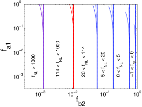
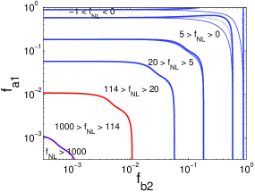
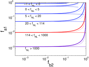
Figure 1: $f_{\rm{NL}}(f_{b2},f_{a1})$ for $\beta=\infty$ (left panel), $\beta=1$ (middle panel), and $\beta=0$ (right panel). The energy density ratio of the first curvaton at the first decay is set to $f_{b1}=0$ (thick solid lines) or $f_{b1}=f_{b2}/2$ (dotted lines) or $f_{b1}=(1+f_{a1}/3)f_{b2}$ (thin solid lines) which corresponds to the simultaneous decay of $a$ and $b$. Contours of equal $f_{\rm{NL}}$ are shown, from left to right (or from bottom to top), for $f_{\rm{NL}}=$ $1000$, $114$, $20$, $5$, $0$, and $-1$.

References

References

- [1] S. Mollerach, Phys. Rev. D 42, 313 (1990); A. D. Linde and V. F. Mukhanov, Phys. Rev. D 56, 535 (1997).
- [2] K. Enqvist and M. S. Sloth, Nucl. Phys. B 626, 395 (2002); D. H. Lyth and D. Wands, Phys. Lett. B 524, 5 (2002); T. Moroi and T. Takahashi, Phys. Lett. B 522, 215 (2001).
- [3] K. Enqvist, H. Kurki-Suonio and J. Valiviita, Phys. Rev. D 62, 103003 (2000); K. Enqvist, H. Kurki-Suonio and J. Valiviita, Phys. Rev. D 65, 043002 (2002).
- [4] K. A. Malik, D. Wands and C. Ungarelli, Phys. Rev. D 67, 063516 (2003); F. Ferrer, S. Rasanen and J. Valiviita, JCAP 0410, 010 (2004); T. Multamaki, J. Sainio and I. Vilja, arXiv:0710.0282 [astro-ph]; Ibid., arXiv:0803.2637 [astro-ph].
- [5] H. Kurki-Suonio, V. Muhonen and J. Valiviita, Phys. Rev. D 71, 063005 (2005); R. Keskitalo, H. Kurki-Suonio, V. Muhonen and J. Valiviita, JCAP 0709, 008 (2007).
- [6] D. H. Lyth, K. A. Malik and M. Sasaki, JCAP 0505, 004 (2005); G. I. Rigopoulos and E. P. S. Shellard, Phys. Rev. D 68, 123518 (2003); D. Langlois and F. Vernizzi, Phys. Rev. D 72, 103501 (2005).
- [7] M. Sasaki, J. Valiviita and D. Wands, Phys. Rev. D 74, 103003 (2006).
- [8] H. Assadullahi, J. Valiviita and D. Wands, Phys. Rev. D 76, 103003 (2007).
- [9] K. Y. Choi and J. O. Gong, JCAP 0706, 007 (2007).