Multirate Synchronous Sampling of Sparse Multiband Signals

Abstract

Recent advances in optical systems make them ideal for undersampling multiband signals that have high bandwidths. In this paper we propose a new scheme for reconstructing multiband sparse signals using a small number of sampling channels. The scheme, which we call synchronous multirate sampling (SMRS), entails gathering samples synchronously at few different rates whose sum is significantly lower than the Nyquist sampling rate. The signals are reconstructed by solving a system of linear equations. We have demonstrated an accurate and robust reconstruction of signals using a small number of sampling channels that operate at relatively high rates. Sampling at higher rates increases the signal to noise ratio in samples. The SMRS scheme enables a significant reduction in the number of channels required when the sampling rate increases. We have demonstrated, using only three sampling channels, an accurate sampling and reconstruction of 4 real signals (8 bands). The matrices that are used to reconstruct the signals in the SMRS scheme also have low condition numbers. This indicates that the SMRS scheme is robust to noise in signals. The success of the SMRS scheme relies on the assumption that the sampled signals are sparse. As a result most of the sampled spectrum may be unaliased in at least one of the sampling channels. This is in contrast to multicoset sampling schemes in which an alias in one channel is equivalent to an alias in all channels. We have demonstrated that the SMRS scheme obtains similar performance using 3 sampling channels and a total sampling rate 8 times the Landau rate to an implementation of a multicoset sampling scheme that uses 6 sampling channels with a total sampling rate of 13 times the Landau rate.

The authors are with the Technion—Israel Institute of Technology, Haifa 32000, Israel (e-mail: mikef@tx.technion.ac.il; eeamir@tx.technion.ac.il; alinden@ee.technion.ac.il; horowitz@ee.technion.ac.il).

1 Introduction

In many applications of radars and communications systems it is desirable to reconstruct a multiband sparse signal from its samples. When the carrier frequencies of the signal bands are high compared to the overall signal width, it is not cost effective and often it is not feasible to sample at the Nyquist rate. It is therefore desirable to reconstruct the signal from samples taken at rates lower than the Nyquist rate. There is a vast literature on reconstructing signals from undersampled data [2]$-$[5]. Most of methods are based on a multicoset sampling scheme.

In a multicoset sampling scheme $m$ low-rate cosets are chosen out of $L$ cosets of samples obtained from time uniformly distributed samples taken at a rate $F$ where $F$ is greater or equal to the Nyquist rate $F_{nyq}$ [3]. In each channel the sampling is offset by a different predetermined integer multiple of the reciprocal of the rate $F$. The data from the different sampling channels are then used to reconstruct a signal by solving a system of linear equations. Under certain conditions on the sampling rate and number of channels, a proper choice of the time offsets ensures that the equations have a unique solution in case that the signal bands are known a priori [3], or unknown a priori [5].

A previous work has demonstrated a different scheme for reconstructing sparse multiband signals [9]. The scheme, called multirate sampling (MRS), entails gathering samples at $P$ different rates. The number $P$ can be small and does not depend on any characteristics of a signal. The approach is not intended to obtain the minimum sampling rate. Rather, it is intended to reconstruct signals accurately with a very high probability at an overall sampling rate significantly lower than the Nyquist rate under the constraint of a small number of channels.

The reconstruction method in [9] does not require synchronization of the different sampling channels. In addition to reducing the complexity of the sampling hardware, unsynchronized sampling relaxes the stringent requirement in multicoset sampling schemes of a very small timing jitter in the sampling time of the channels. Simulations have indicated that MRS reconstruction is robust both to different signal types and to relatively high noise.

Accurate signal reconstruction using the unsynchronized MRS scheme of [9] requires that each frequency in the support of the signal be unaliased in at least one of the sampling channels. In this paper we describe a new reconstruction algorithm that overcomes this deficiency by using synchronized sampling channels. In our synchronized multirate sampling (SMRS) scheme, the aliasing is resolved, in the same spirit as multicoset sampling schemes, by solving a system of linear equations. Therefore, the SMRS scheme enables the reconstruction of signals that cannot be reconstructed using MRS scheme.

In our SMRS scheme each sampling rate must be an integer multiple of the same basic frequency. The reconstruction method in our SMRS scheme requires the same frequency resolution in all sampling channels despite the fact that the sampling rate is different in each channel. This requirement is well suited to the implementation of the scheme using the optical system described in [10]. The sampling is performed in two steps. In the first step the entire signal spectrum is downconverted into a low frequency region called baseband by multiplying the signal with a train of short optical pulses [10]. In each of the sampling channels the pulse rate is different. The frequency downconverted analog signals are then converted in each sampling channel to digital signals using an A/D electronic converter that samples at the highest of the channel rates. The result is that the signal is sampled in all channels with the same time resolution that is determined by the sampling rate of the A/D converter. Alternatively, since each sampling rate must be an integer multiple of the same basic frequency, a common frequency resolution can be obtained by using the same time window for all channels.

There is an inherent advantage to sampling, in each channel, near the maximum sampling rate made possible by cost and technology. This is because sampling at higher rates increases the signal to noise ratio in sampled signals [9]. Our simulation results indicate that when the sampling rate in each channel increases, our SMRS scheme requires significantly fewer sampling channels than does a multicoset sampling scheme of [5] to obtain comparable reconstruction success. When the sampling rate in each channel increases, the probability that a sparse signal aliases simultaneously in all sampling channels becomes very low in an MRS scheme. It is lower than in a multicoset sampling scheme in which, because all channels sample at the same frequency, an alias in one channel is equivalent to an alias in all channels. Our numerical simulations indicate that the success rate of our SMRS scheme is significantly higher than that of a multicoset sampling schemes of [5] when the number of sampling channels is small (3 in our simulations) and the sampling rate of of each channel is high.

Exactly the same data obtained in the SMRS scheme can be obtained using a multicoset sampling scheme. However the multicoset pattern requires many more channels, each of which samples at a very low rate. In a numerical example of section 5 a 3 channel multirate sampling pattern is equivalent to a 58 channel multicoset sampling pattern. With this multicoset pattern the time difference between two consecutive samples is on the order of 1 psec. Such an accuracy cannot be practically achieved.

In an SMRS scheme the data is reconstructed differently than in a multicoset scheme implementation of [5]. In this multicoset recovery scheme it is assumed that, in addition to being sparse, the spectrum of the signal consists of bands each of which is narrower than the coset sampling rate. However, our SMRS scheme requires no such assumptions on the originating signal. The reconstruction of sparse signals in our SMRS scheme is robust. This is because most of the sampled spectrum is unaliased in at least one of the sampling channels. This is in contrast to the equivalent multicoset sampling scheme with many low rate sampling channels in which the alias probability is very high and an alias in one channel is equivalent to an alias in all channels. In such cases a blind signal recovery of [5] can be found only by using a pursuit algorithm whereas, in many cases, the SMRS scheme doesn’t require a pursuit algorithm. The signal is reconstructed directly by a single matrix inversion. By making a very reasonable physical assumption, we are also able to simplify the reconstruction by reducing the number of possible signal locations in a straightforward manner.

The SMRS scheme reconstructs signals by solving a system of linear equations. Our simulations indicate that linear equations in an SMRS scheme are numerically stable in that they have low condition numbers. This makes them rather insensitive to noise. In the SMRS scheme, when sampling at total sampling rate that is significantly higher than theoretically required, the probability that part of the signal spectrum will not be aliased in at least one of the sampling channels is very high. The unaliased parts of the signal can be recovered directly from the sampling channels. Our simulation results indicate that the sensitivity of the reconstructed signal to noise added at frequencies of baseband that are not aliased in at least one of sampling channels is very low.

2 Synchronized MRS

In this section we describe the SMRS scheme. Let $F_{\textrm{max}}$ be an assumed maximum carrier frequency and let $X(f)\in L^{2}([0,F_{\textrm{max}}])$ be the Fourier transform of a complex-valued signal $x(t)$ that is to be reconstructed from its samples. Throughout the analysis we normalize the Fourier transform by

$$X(f)=\int_{-\infty}^{\infty}x(t)e^{-j2\pi ft}\;dt.$$

The modifications required to reconstruct real-valued signals are described in the Appendix. We assume that the signal $x(t)$ to be sampled, in addition to being bandlimited in $[0,F_{\textrm{max}}]$, is multiband; i.e., the support of its spectrum is contained within a finite disjoint union of intervals $(a_{n},b_{n}]$, each of which is contained in $[0,F_{\textrm{max}}]$. By assumption, $\max{b_{n}}\leq F_{\textrm{max}}$. In reconstructing a signal we do not assume any a priori knowledge of the number or location of the intervals $(a_{n},b_{n}]$. The only requirement is that the signal be sparse; i.e., that for a signal whose spectral support is contained within the $N$ intervals $(a_{i},b_{i}]$, $\sum_{k=1}^{N}b_{k}-a_{k}\ll F_{\textrm{max}}$.

In the MRS scheme of [9] a signal is sampled at $P$ different sampling rates $F^{i}$ ($i=1\ldots P$). If the delays of the channels are denoted by $\Delta^{i}$, the sampled signals $x^{i}(t)$ are given by

$$x^{i}(t)=x(t)\sum_{n=-\infty}^{\infty}\delta\left(t-\frac{n}{F^{i}}-\Delta^{i}\right)$$ (1)

where $\delta(t)$ is a dirac delta “function”. The spectrum $X^{i}(f)$ of the sampled signal in the $i$th channel satisfies

$$X^{i}(f)=F^{i}\sum_{n=-\infty}^{\infty}X(f+nF^{i})\exp[j2\pi(f+nF^{i})\Delta^{i}].$$ (2)

Since the channels are synchronized in time, we may set each $\Delta^{i}=0$. Equation (2) becomes

$$X^{i}(f)=F^{i}\sum_{n=-\infty}^{\infty}X(f+nF^{i}).$$ (3)

It follows from (3) that all the information about the $i$th sampled spectrum $X^{i}(f)$ is contained in the interval $[0,F^{i}]$. This interval is called the $i$th baseband. To process the sampled signals it is necessary to discretize the frequency axis. We use the same frequency resolution ($\Delta f$) in all of the sampling channels. The same frequency resolution is directly obtained if the system is implemented using an optical sampling system [10]. To use our reconstruction method each sampling rate should be chosen to be an integer multiple $M^{i}$ of the basic frequency resolution: $F^{i}=M^{i}\Delta f$. By using a sampling time window with a duration $T=1/\Delta f$, the same frequency resolution $\Delta f$ is obtained in all of the sampling channels. Alternatively, the same frequency resolution can be obtained in an optical system by using A/D converters with the same rate at the output of all the optical downconvertors [10]. To reduce computational requirements we ignore redundant data. Thus, only $M^{i}$ entries of the Discrete Fourier transform (DFT) are retained for further processing.

We represent the signals over the common discretized frequency axis with the following notations:

$$X^{i}[k] = X^{i}(k\Delta f),\;\;k=0,\ldots,M^{i}-1,$$

$$X[k] = X\;(k\Delta f),\;\;k=0,\ldots,M-1\,,$$

where $\Delta f$ is the frequency resolution, $M=\lceil F_{\textrm{max}}/\Delta f\rceil$, $X^{i}[k]$ is the spectrum of the sampled data from the discretized frequencies in the baseband $[0,F^{i}]$ and $X[k]$ is the spectrum of the originating signal at the discretized frequencies. Equation (3) takes the form

$$X^{i}[k]=F^{i}\sum_{l=0}^{M-1}X[l]\sum^{\infty}_{n=-\infty}\delta[l-(k+nM^{i})]$$ (4)

where $\delta[n]$ is the Kronecker delta function. Equation (4) can be written in matrix form as follows:

$$\textbf{x}^{i}=\textbf{A}^{i}\textbf{x}$$ (5)

where $\textbf{x}^{i}$ and x are given by

$$(\textbf{x}^{i})_{k+1} =X^{i}[k],~{}~{}0\leq k\leq M^{i}-1,$$ (6)

$$(\textbf{x})_{k+1} =X[k]~{}~{}0\leq k\leq M-1,$$

and $\textbf{A}^{i}$ is a $M^{i}\times M$ matrix whose elements are given by

$$\textbf{A}_{k+1,l+1}^{i}=F^{i}\sum^{\infty}_{n=-\infty}\delta[l-(k+nM^{i})].$$ (7)

Each element $\textbf{A}_{k,l}^{i}$ is equal to either $F^{i}$ or 0. This is because there is at most one contribution in the infinite sum of $\delta$’s which is made when $l\equiv k(\mod M^{i})$. In each row of the matrix $\textbf{A}^{i}$ there are only $\lfloor F_{\max}/F^{i}\rfloor$ non zero elements.

For each value of $i$ ($i=1\ldots P$), (5) defines a set of linear equations that relate the spectrum of the signal to the spectrum of its samples. The vector x in (5) is the same for all the $P$ equations because it doesn’t depend on the sampling.

The vector $\widehat{\textbf{x}}$ and the matrix $\widehat{\textbf{A}}$ are obtained by concatenating the vectors $\textbf{x}^{i}$ and matrices $\textbf{A}^{i}$ as follows:

$$\widehat{\textbf{x}}=\left(\begin{array}[]{ccc}\textbf{x}^{1}\\ \textbf{x}^{2}\\ \vdots\\ \textbf{x}^{P}\par\end{array}\right),~{}\widehat{\textbf{A}}=\left(\begin{array}[]{ccc}\textbf{A}^{1}\\ \textbf{A}^{2}\\ \vdots\\ \textbf{A}^{P}\end{array}\right).$$ (16)

These form the system of equations

$$\widehat{\textbf{x}}=\widehat{\textbf{A}}~{}\textbf{x}.$$ (17)

The matrix $\widehat{\textbf{A}}$ has exactly $P$ non-vanishing elements in each column that correspond to the locations of the spectral replica in each channel baseband.

In case that the signal is real-valued its spectrum fulfills

$$X(f)=\overline{X}(-f)$$ (18)

where $\overline{a+bj}=a-bj$ is the complex conjugate. The equations for reconstructing such a signal are described in the Appendix.

To invert (17) and calculate the discretized signal spectrum (x) it is necessary that the number of rows $\sum_{i=1}^{P}M^{i}$ in A be equal to or larger than the number of columns $M$. Defining $F_{\textrm{total}}=\sum_{i=1}^{P}F^{i}$ makes this condition equivalent to the condition

$$F_{\textrm{total}}>F_{\textrm{max}}.$$ (19)

The condition on the sampling rates given in (19) is consistent with the requirement that the sampling rate be greater than the Nyquist rate of a general signal whose spectral support is $[0,F_{\textrm{max}}]$. However, when sampling sparse signals, an inversion of the matrix may be possible even if the condition (19) is not fulfilled. Our objective is to invert (17) in the case of sparse signals with sampling rates $F_{\textrm{total}}<F_{\textrm{max}}$.

3 Inversion Algorithm

In this section we describe our inversion algorithm for the SMRS scheme. The purpose of the algorithm is to invert (17); i.e., to calculate the vector x from the vector $\widehat{\textbf{x}}$. To invert the equations with sampling rates lower than those prescribed by (19) the assumption that the signal is sparse should be taken into account.

3.1 Known Band Locations

In the case in which the signal band locations $(a_{n},b_{n}]$ are known (17) can be simplified easily. All the elements of x that correspond to the frequencies not in the spectral support $\cup_{n}(a_{n},b_{n}]$ are eliminated from (17). All the columns of the matrix which correspond to these elements are also eliminated. The reduced system of equations that corresponds to (17) is given by

$$\widehat{\textbf{x}}_{\textrm{red}}=\widehat{\textbf{A}}_{\textrm{red}}\textbf{x}_{\textrm{red}}.$$ (20)

A unique solution exists only if $\widehat{\textbf{A}}_{\textrm{red}}$ is full column rank. In this case the inverse can be found using the Moore-Penrose pseudo-inverse [12]. In a matrix of full column rank the number of rows must equal or exceed the number of columns.

Although the entire spectrum is downconverted to baseband, we assume that we are sampling highly sparse signals. Hence the number of non-zero entries in each $\textbf{x}^{i}$ is significantly smaller than $M^{i}$ in at least one of the sampling channels. The number of non-zero entries in each $\textbf{x}^{i}$ might even be smaller because of aliasing. A necessary condition for a unique inverse or pseudo-inverse of $\widehat{\textbf{A}}_{\textrm{red}}$ is that this number still be greater than the number of non-zero entries of x. This is consistent with a Landau theorem [1] that states that one cannot reconstruct a signal if the spectral density of the samples collected from all sampling channels is less than the spectral support of the originating signal.

The choice of sampling rates imposes restrictions on the possible values of $F_{\max}$ for which an inversion of (20) is possible. For the matrix $\widehat{\textbf{A}}_{\textrm{red}}$ to have full column rank, it must not have any identical columns. Since we do not restrict the possible locations of the known signal bands, any combination of columns of the matrix $\widehat{\textbf{A}}$ may appear in the matrix $\widehat{\textbf{A}}_{\textrm{red}}$. Therefore we require that $\widehat{\textbf{A}}$ not have any identical columns. The matrix $\widehat{\textbf{A}}$ is composed of $P$ sub-matrices $\textbf{A}^{i}$ whose columns are periodic:

$$\textbf{A}_{k,l+M^{i}}^{i}=\textbf{A}_{k,l}^{i}.$$

For the matrix $\widehat{\textbf{A}}$ not to be periodic, it is required that any common period of the $P$ sub-matrices be larger than $M$. This condition is met if the least common multiple of the $\{M^{i}\}_{i}$ is larger than $M$. As a result, $F_{\max}$ should fulfill $F_{\max}<lcm(M^{1},\ldots,M^{P})\Delta f$, where $lcm$ denotes least common multiple.

3.2 Unknown Bands’ Location

In the case that the locations of the bands $(a_{n},b_{n}]$ are not known a priori some additional assumptions must be made. In the multicoset recovery scheme of [5] it was assumed that the maximum band width is known a priori. In our SMRS scheme we do not make any assumptions on the intervals $(a_{n},b_{n}]$ but instead we add assumptions on a signal’s spectrum itself.

We assume that, for each discretized frequency $k\Delta f$, any sampled spectrum $X^{i}(k\Delta f)=0$ is due only to lack of a signal in any of its replicas and not due to any aliasing. In other words if, for any $n$, $X(f+nF^{i})\neq 0$, then $X^{i}(f)\neq 0$. Another assumption is that there is a unique solution in the case the signal support is known, i.e., the matrix $\widehat{\textbf{A}}_{\textrm{red}}$ has a full column rank for a known support.

Applying the first assumption, one can detect baseband frequencies in which there is no signal. These frequencies can be eliminated in the reduction of (17). We describe this simple procedure for eliminating frequencies which, according to our assumption, cannot be part of the spectral support of the originating signal. The elimination is similar to one presented in asynchronous-MRS [9]. We denote the indicator function $\chi^{i}[l]$ as follows:

$$\chi^{i}[l]=\left\{\begin{array}[]{lll}1,&&\mathrm{for\;all\;}l\in[0,M-1]\text{\;such that\;}X^{i}(l\Delta{f})\neq 0\\ 0,&&\mathrm{otherwise}.\end{array}\right.$$ (21)

The function $X^{i}(f)$ is periodic with period $F^{i}$. Therefore $\chi^{i}[l]$ is a periodic extension of an indicator function over the baseband $f\in[0,F^{i})$.

We define the $\chi[l]$ as follows:

$$\chi[l]=\prod_{i=1}^{P}\chi^{i}[l],~{}~{}~{}~{}l\in[0,M-1].$$ (22)

The function $\chi[l]$ equals 1 over the intersection of all the upconverted bands of the $P$ sampled signals and it defines the columns of the matrix $\widehat{\textbf{A}}$ that are retained in forming the reduced matrix $\widehat{\textbf{A}}_{\textrm{red}}$. All other columns are eliminated and their corresponding elements in the vectors x are also eliminated. After the elimination of the columns from the matrix $\widehat{\textbf{A}}$, the matrix rows which correspond to zero elements in $\widehat{\textbf{x}}$ and their corresponding elements in the vectors $\widehat{\textbf{x}}$ are also eliminated. In some cases the function $\chi[l]$ equals 1 only for frequencies within the spectral support of the signal. In such cases the resulting equations are identical to those found in the previous subsection (equation (20)). However, in other cases, $\chi[l]$ may also equal 1 for frequencies outside the signal’s true spectral support. In such cases the reduced matrix will have more columns than the matrix in the case in which the spectral support of the signal is known. As a result the inversion requires finding the values of more variables.

Each eliminated zero energy baseband component causes elimination of respective rows and columns. The elimination of one baseband entry means that all the frequencies that are downconverted to that baseband entry (the aliasing frequencies) are also eliminated. This is because of our first assumption that zero entry in the baseband corresponds to zero entries in all of the frequency components of the original signal that are down-converted to frequency of the baseband entry. Therefore, elimination of one baseband entry results in elimination of $\lfloor F_{\max}/\min\{F^{i}\}\rfloor$ to $\lceil F_{\max}/\max\{F^{i}\}\rceil$ corresponding columns. Thus, if the number of the zero elements in $\widehat{\textbf{x}}$ is sufficiently large, the number of rows in the matrix $\widehat{\textbf{A}}_{\textrm{red}}$ may be larger than the number of columns.

If in addition, matrix $\widehat{\textbf{A}}_{\textrm{red}}$ has a full column rank, the problem is either consistent or overdetermined. In such cases there is a unique inversion to (20) which can be found using the Moore-Penrose pseudo-inverse. If the matrix is not full column rank, the problem is underdetermined and the inversion is not unique. A unique solution in such cases can be obtained either by increasing the total sampling rate or by adding additional assumptions on the signal.

3.3 Ill-posed cases

In many cases the matrix in (20) for unknown band locations is not full column rank. In these cases there are subsets of columns in the matrix $\widehat{\textbf{A}}_{\textrm{red}}$ that are linearly dependent. Using this linear dependence, a solution to (20) can be found. However any solution found can be used to construct an infinite number of solutions to the equation. Thus, there is no unique inversse to (20) and the inversion problem is ill-posed.

To reconstruct a signal in the case in which the inversion problem is ill-posed we impose an additional assumption on the signal. We assume that in the case the signal support is unknown and the problem is ill-posed, among all possible solutions to (20), the originating signal is the one that is composed of the minimum number of bands. This is the signal we attempt to construct. We also assumed earlier that the reduced matrix which corresponds to the case in which the signal support is known is well-posed. In case that this assumption is not fulfilled the sampled signal does not contain enough information for solving the problem.

Under the three assumptions stated above (the assumption that leads to matrix reduction, the existence of the unique solution to (20) when the signal bands are known, and band-sparsity) the inversion problem is reduced to finding the solution of (20) that is composed of the minimum number of bands. The problem is NP-complex since we need to test every possible combination of bands.

The algorithm described here is of lower complexity and its purpose is to find a solution of (20) that is composed of the minimum number of bands without testing all the combinations. The resulting algorithm attains a lower success rate but decreases the run-time significantly as compared to an NP-complex algorithm. We do not provide the conditions under which the correct solution is obtained.

Our algorithm is based on the $Orthogonal~{}Matching~{}Pursuit~{}(OMP)$ [8]. This algorithm belongs to the category of the ”Greedy Search” algorithms. The original OMP algorithm is used to find the sparsest solution x of underdetermined equations $\textbf{A}\textbf{x}=\textbf{b}$ [8] where A is an underdetermined matrix. The sparsest solution is the solution having the smallest norm $\|\textbf{x}\|_{0}$ where $\|\textbf{x}\|_{0}$ is the number of non zero elements in the vector x. The original OMP algorithm collects columns of the matrix A iteratively to construct a reduced matrix $\textbf{A}_{\textrm{r}}$. At each iteration $n$ the column of A which is added to $\textbf{A}^{n-1}_{\textrm{r}}$ to produce a matrix $\textbf{A}^{n}_{\textrm{r}}$ is the column which results in the smallest residual error $\min_{\textbf{x}}\|\textbf{b}-\textbf{A}^{n}_{\textrm{r}}\textbf{x}\|^{2}_{2}$ where for every vector y, $\|\textbf{y}\|^{2}_{2}=\sum_{i}y^{2}_{i}$. The iterations are stopped when some threshold $\epsilon$ is achieved. Sufficient conditions are given for the algorithm to obtain the correct solution [8].

We denote $\textbf{A}=\widehat{\textbf{A}}_{\textrm{red}}$, $\textbf{b}=\widehat{\textbf{x}}_{\textrm{red}}$ and $\textbf{x}=\textbf{x}_{\textrm{red}}$. Since we are seeking the solution of $\textbf{A}\textbf{x}=\textbf{b}$ with the smallest number of bands and not the smallest norm $\|\textbf{x}\|_{0}$, we modify the OMP algorithm by instead of choosing a single column as in [8] by selecting iteratively blocks of possible locations. The columns of the matrix A fall into $J$ blocks. Each block is indexed by $j$ and $B_{j}$ contains the index of columns of the $j$th block.

Each index set $B_{j}$ identifies a possible band of the spectral support of the reconstructed signal. We start the iteration with the empty set $S^{0}=\emptyset$ of column indexes, the empty matrix $\textbf{A}^{0}_{\textrm{r}}$, and the set $B^{0}=\bigcup_{j=1}^{J}B_{j}$, so that at $n$th iteration the following holds: $S^{n}\bigcup B^{n}=B^{0}$. At the $n$th iteration $(n>1)$ the algorithm must decide which block to add to $\textbf{A}^{n-1}_{\textrm{r}}$. If the index set $B_{j}$ is chosen, then $S^{n}=S^{n-1}\cup B_{j}$ and $B^{n}=B^{n-1}\setminus B_{j}$. The matrix $\textbf{A}^{n}_{\textrm{r}}$ is the matrix whose columns are selected from A according to the indexing set $S^{n}$.

The block added is the one that produces the smallest residual error $\epsilon^{n}=\min_{B_{j}\in~{}B^{n-1}}\min_{\textbf{x}}\|\textbf{b}-\textbf{A}^{n}_{\textrm{r,j}}\textbf{x}\|^{2}_{2}$ where $\textbf{A}^{n}_{\textrm{r,j}}$ is the matrix obtained by adding the block indexed by $B_{j}$ to $\textbf{A}^{n-1}_{\textrm{r}}$. The algorithm stops when the threshold $\epsilon$ is reached. The threshold $\epsilon$ is a very small number and reflects upon the finite numerical precision of the calculations.

The algorithm performed well in our simulations. However, there were cases in which the support of the reconstructed solution did not contain all the originating bands and cases in which the reconstructed signal was incorrect even though all the assumptions on a signals given in section 3.2 were fulfilled. Only after performing the last step of the algorithm is it possible to determine the support of the signal. The algorithm failed primarily for one of two reasons. One of them was due to the inclusion of a block that reduced the residual error on one hand but on the other hand, caused a resulting matrix $\textbf{A}^{n}_{\textrm{r}}$ to be not full column rank as hypothesized in our problem (in section 3.2). This can happen, for example, when a block consists of a correct sub-block and erroneous sub-blocks. Including any erroneous sub-blocks may result in an ill-posed problem. Another reason for failure was a large dynamic range of the signals. When reconstructing such signals, correct bands may be ignored by the algorithm in cases that the energy within the bands is significantly lower than the energy in other bands.

Sufficient conditions that assure that the algorithm converges to a unique solution have not yet been determined.

4 Simulations results

The ability of the signal reconstruction algorithm to recover different types of signals was tested. In one set of simulations the ability of the algorithm to reconstruct multiband complex and real-valued signals with different spectral supports, shapes, and band widths that were not known a priori was tested. Additional simulations were performed in which real-valued multiband signals were contaminated by additive white noise. Band carrier frequencies were chosen from a uniform distribution over the maximum support: 0-20 GHz for complex signal and $-20$ to $20$ GHz for real-valued signals. For each set of simulations we counted the mean rate of ill-posed cases in which the modified OMP algorithm was used to recover the signal. Mean times for accurate signal reconstruction were also recorded. Failures of the reconstruction were either because one of the initial assumptions was not fulfilled or because of the failure of the modified OMP algorithm.

In different simulations the width of each band (hence the total bandwidth of the signal) was varied. The number of bands was always set equal to 4 for complex signals and to 8 for real-valued signals (4 positive bands and 4 negative bands). However, the reconstruction algorithm was unaware of this number. In all the simulations the frequency resolution was set to 5 MHz. The simulations were performed on a 2 GHz Core2Duo CPU with 2 GB RAM storage in the MATLAB 7.0 environment (no special programming was performed to use both cores).

4.1 Ideal multiband signals

In the case of ideal multiband signals, because of the absence of energy outside of strictly defined bands, one can expect a perfect reconstruction. Accordingly, the algorithm was evaluated by a perfect reconstruction criterion; i.e., a mean difference between the true and the reconstructed signal spectrum less than $10^{-10}$. Whenever this error was attained, the reconstruction was deemed to have been successful. Otherwise, it was deemed to have failed. The threshold for the modified OMP was chosen accordingly; $\epsilon=10^{-20}$.

Simulations were carried out for complex signals to compare the results to those published using the multicoset sampling recovery scheme of [5]. The sampling rates were chosen to be 0.95, 1.0 and 1.05 GHz yielding a total sampling rate $F_{\textrm{total}}=3.0$ GHz.

Different signals with 4 bands of equal width were generated. Each band was chosen to lie within the interval $[0,20]$ GHz. Both the real and imaginary spectra of the signal within each band were chosen to be normally distributed. Specifically, for each frequency $f=k\Delta f$ in a chosen band, the real and imaginary components of $X(f)$ were chosen randomly and independently from a standard normal distribution. Each bands’ spectra were scaled by a constant $\alpha$ such that each bands’ energy was equal to a uniformly generated value $E$ on the interval $[1,5]$; i.e., for specific band,

$$X(f)=\alpha[X_{r}(f)+jX_{im}(f)],~{}\|X(f)\|_{2}=E.$$

These signals were also used to test the multicoset sampling reconstruction scheme of [5]. The empirical success rates were obtained from 1000 runs, each with a different total bandwidth ($F_{\textrm{Landau}}$). The success rate is shown in Fig. 1. We have validated that the empirical success rate did not significantly change when the number of simulation runs was increased from 1000 to 5000.

As is evident from Fig. 1, the empirical success percentage of an ideal reconstruction is high when $F_{\textrm{total}}/F_{\textrm{Landau}}\geq 5$. In the SBR2 scheme (downsampling factor $L=199$) in [5] the empirical success rate shows perfect reconstruction for at least $p=14$ channels. This corresponds to $F_{\textrm{total}}=p/LT=1.4$ GHz and hence $F_{\textrm{total}}/F_{\textrm{Landau}}$ should be greater than about 3. Although the total sampling rate in [5] is lower than in SMRS, the number of channels that are used in that scheme is significantly higher compared to that used in SMRS where only 3 channels are used.

Another simulation in [5] shows that for lower number of channels with $L=23$ empirical perfect reconstruction is achieved with at least 6 channels and $F_{\textrm{total}}/F_{\textrm{Landau}}>13$. In the SMRS scheme empirical perfect reconstruction was obtained using only three channels with a total sampling rate $F_{\textrm{total}}/F_{\textrm{Landau}}\geq 5$. The system parameters (number of sampling channels, sampling rates, $F_{\max}$) that were used in our last simulation are the same as those used in our optical sampling experimental set up. The fact that the simulation results were obtained in a practical situation demonstrates that our SMRS scheme can reconstruct sparse signals perfectly using both a fewer number of sampling channels and with a lower total sampling rate than are required by multicoset sampling schemes.

We note that the same data that is obtained in a SMRS pattern can always be obtained by a multicoset sampling pattern since the ratio between each pair of sampling rates is rational. In our example the sampling rate of each coset is equal to $1/{LT}=50$ MHz. The number of multicoset sampling channels ($p$) is 58. The time offset between the cosets is a multiple of $T=\frac{1}{399~{}GHz}$. The downsampling factor $L$ is $399$ GHz$/50$ MHz$=$7980. Note that since $L$ is not prime, we are not guaranteed to obtain a universal sampling pattern [5].

Fig. 1 shows that in our scheme 100 percent empirical success was obtained for $F_{\textrm{total}}/F_{\textrm{Landau}}>5$. This corresponds to a maximum overlap in a coset scheme of $K=16$ and hence $p/K=3.6$ for $p=58$. In comparison, for $p=14$ channels and downsampling factor of $L=199$ in a multicoset sampling scheme in [5], the empirical success rate of 100 percent was obtained for SBR2 algorithm for $p/N=3.5$. This ratio is similar to the equivalent ratio obtained in our scheme (3.6) although the downsampling factor in our equivalent multicoset scheme is equal to 7980. For approximately 95 percent success rate in SBR2 scheme of [5], the ratio $p/N$ is 2.75. In our scheme, for the same empirical success rate of 95 percent, $F_{\textrm{total}}/F_{\textrm{Landau}}=3.53$ and the equivalent ratio of the number of channels to maximal number of overlaps is $p/K=2.4$.

The mean percentage of ill-posed cases is shown in Fig. 2. The figure shows that for $4\leq F_{\textrm{total}}/F_{\textrm{Landau}}\leq 10$, in most of the tested cases the inversion was ill posed. Nonetheless, a very high success percentage was obtained for these values. This indicates that our modified OMP algorithm was very successful in resolving these cases.

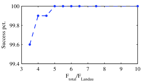
Figure 1: Empirical success percentages for 4-bands complex signals for different spectral supports ($F_{\textrm{Landau}}$) with $F_{\textrm{Nyquist}}$=20 GHz, total sampling rate $F_{\textrm{total}}=3$ GHz

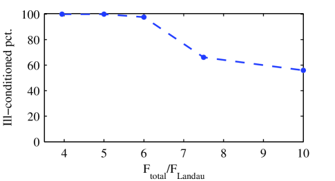
Figure 2: Ill-posed cases mean percentage for 4-bands complex signals for different spectral supports ($F_{\textrm{Landau}}$) with $F_{\textrm{Nyquist}}$=20 GHz, total sampling rate $F_{\textrm{total}}=3$ GHz

Fig. 3 shows the mean run time as a function of $F_{\textrm{total}}/F_{\textrm{Landau}}$ (constant total sampling rate and varying signal support). Because matrix inversion is the most computationally intensive operation in the algorithm, mean run time decreases with a reduction in signal bandwidth. This is because, with a fixed resolution, matrix size is proportional to signal bandwidth. Moreover, as the ratio $F_{\textrm{total}}/F_{\textrm{Landau}}$ increases, the possible spectral support obtained at the first step of the reconstruction increases beyond the increase of the signal bandwidth.

We note that we could reduce the run time without significantly affecting the empirical success percentage by solving (17) using a low resolution and reconstructing the signal using a higher resolution.

The algorithm, modified as explained in the Appendix, was also tested against real-valued signals. The assumed maximum frequency $F_{\max}$ was set to $20$ GHz. The number of sampling channels was set to 3 with the sampling frequencies chosen to be $F^{1}=3.8$ GHz, $F^{2}=4.0$ GHz, and $F^{3}=4.2$ GHz resulting in a total sampling rate, $F_{\textrm{total}}=12$ GHz. The sampling frequencies are the same as are used in our experiments based on asynchronous MRS [9]. The number of bands was set to $8$ ($4$ positive and $4$ negative frequencies, assuming no carrier frequency so low as to have the $0$ frequency in its spectrum). Each band was chosen to be of equal width $F_{\textrm{Landau}}/8$.

Once a band $(a,b]$ was chosen, the spectrum of $X(f)$ for $f\in(a,b]$ was determined by the following formula:

$$X(f)=A\sin\left[\frac{\pi(f-a)}{b-a}\right]e^{j\theta}.$$

The phase $\theta$ was chosen randomly from a uniform distribution on $[0,2\pi]$ and the amplitude $A$ was chosen randomly from a uniform distribution on $[1,1.2]$.

Fig. 4 shows the empirical success percentages of the algorithm tested against real valued signals. As is evident from the figure, the empirical success percentage is high when $F_{\textrm{total}}/F_{\textrm{Landau}}\geq 8$. We note that the required sampling rate is significantly higher in this example than in the complex signals simulation. The reason is that in our real case example there are twice as many bands as in the complex case simulations. Hence, after the sampling, an overlap may also occur between the negative and the positive bands of the real signal. We note that when sampling a real signal at a sampling rate $F^{i}$, it is sufficient to know the spectrum in a frequency region $[0,F^{i}/2]$. However, for real signals, there is uncertainty as to whether a signal in baseband is obtained from a signal in the positive band or in the negative band.

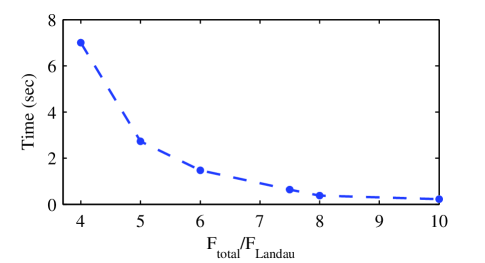
Figure 6: Mean recovery times for equal 4-bands real signals for different spectral supports (total bandwidth) with $F_{\textrm{Nyquist}}$=40 GHz, total sampling rate $F_{\textrm{total}}=12$ GHz

The number of ill-posed cases and the mean recovery run times for the real-valued signals are shown in Figs. 5 and 6 respectively. It can bee seen that the mean rate of ill-conditioned cases is much lower for real-valued signal simulations than for complex ones. This could be due to the correlation between positive and negative frequency components of real signals.

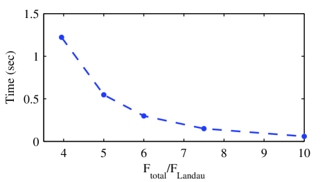
Figure 3: Mean run times for 4-bands complex signals for different spectral supports ($F_{\textrm{Landau}}$) with $F_{\textrm{Nyquist}}$=20 GHz, total sampling rate $F_{\textrm{total}}=3$ GHz

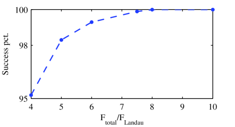
Figure 4: Empirical success percentages for equal 4-bands real signals for different spectral supports ($F_{\textrm{Landau}}$) with $F_{\textrm{Nyquist}}$=40 GHz, total sampling rate $F_{\textrm{total}}=12$ GHz

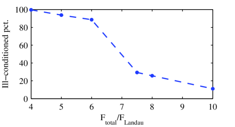
Figure 5: Ill-posed cases mean rate for 4-bands real signals for different spectral supports ($F_{\textrm{Landau}}$) with $F_{\textrm{Nyquist}}$=40 GHz, total sampling rate $F_{\textrm{total}}=12$ GHz

4.2 Solution Stability

The stability of the linear equations used in the recovery scheme was tested via the condition number for the real-valued signals equations ((30) in the Appendix). This case is important in our experiments since we sample real signals [9]. The reconstruction scheme for real-valued signals requires solving two systems of linear equations; one for the real part and the other for the imaginary part. Each of the two systems of equations is described by a different matrix. In each test case we presented the maximum value of the condition numbers of the two matrices. For 4-band 200-MHz-width randomly generated signals ($F_{\textrm{Landau}}$=1.6 GHz) the condition number among 1000 runs was at most 5.3. The condition numbers histogram is shown in Fig. 7.

When sampling a sparse signal, most frequencies of the signal are unaliased in at least one of the sampling channels. It can be easily shown that when a frequency component of the signal is not aliased in any of the sampling channels, the reconstructed signal is obtained simply by averaging the corresponding sampled spectrum at the different sampling channels. The reconstruction of a frequency component that is unaliased in at least one of the sampling channels can also be easily performed by copying the corresponding unaliased spectrum to the reconstructed signal. Therefore, for sparse signals, the reconstruction in the SMRS scheme is robust and the condition number of the matrices is small. Indeed, we have verified that the condition number of the matrix increases as the number of frequencies in the original signal that are aliased increases. Fig.  8 shows the mean values of condition numbers versus number of aliased frequencies as calculated for the 4 real signals each with a 200 MHz width that are sampled at $F_{\textrm{total}}=12$ GHz. The other parameters of the simulation are the same as those in the simulation that resulted in Fig. 4.

4.3 Noisy signals

The algorithm’s performance was also tested for its ability to reconstruct real-valued signals contaminated by Gaussian white noise. The presence of noise demands some modification of the algorithm. One modification is in detecting the possible bands of the support of the originating signal. Because the spectral support of white noise is not restricted to the spectral support of the uncontaminated signal, the indicator functions in (21) cannot be used. Instead, we adapt (21) to noisy cases similarly as in  [9]. In [9], for the indicator function $\chi^{i}[l]$ to be equal to 1 at any frequency, it was required that the average energy of the signal in the neighborhood of that frequency be higher than a certain threshold. In SMRS we further expand each band in $\chi[l]$ to include additional frequencies that might otherwise be omitted when defining the indicator functions $\chi^{i}[l]$. Once the bands are identified the matrix equations are constructed exactly as in the noiseless case.

The solution of the linear equations given in (30) is modified in the noisy case. Because the added white noise affects the entire spectrum, a signal contaminated by white noise can no longer be considered multiband in the strict sense. Thus one cannot expect to reconstruct it perfectly from samples taken at a total rate lower than the Nyquist rate. Whereas in the ideal noiseless case the error norm vanishes, with a signal containing noise, one must relent on a perfect reconstruction and settle for a minimum error. In the noisy case the solution to (30) should solve the least square problem $\min_{\textbf{x}^{\textrm{r,im}}_{\textrm{red}}}\|\widehat{\textbf{x}}^{\textrm{r,im}}_{\textrm{red}}-\widehat{\textbf{A}}^{\textrm{r,im}}_{\textrm{red}}~{}\textbf{x}^{\textrm{r,im}}_{\textrm{red}}\|$. When the the matrix $\widehat{\textbf{A}}^{\textrm{r,im}}_{\textrm{red}}$ is not full column rank, we use the modified OMP algorithm which is adjusted to account for the errors due to noise. As noted above, in the noiseless case, one can expect a perfect reconstruction and thus the threshold error $\epsilon$ can be set to $0$ or a very small number. However, with noisy signals, some care must be taken in choosing $\epsilon$. On the one hand, if the $\epsilon$ is chosen too large, the algorithm may stop before a solution is reached. On the other hand, if $\epsilon$ is chosen too small, the reconstructed signal may include bands that are not in the originating signal. The problem of too high threshold is solved by changing the stop criterion. Instead of stopping the algorithm when a threshold is attained, we check at each iteration whether the block that reduces the residual error the most causes the resulting matrix to be rank deficient. When this occurs, the iteration are stopped and the block is not added to the matrix.

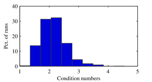
Figure 7: Condition numbers histogram of the mixing matrix in (30) for 4 bands, 200 MHz width real signals, $F_{\textrm{total}}=12$ GHz

An additional change is made to the algorithm when treating the blocks. In the noiseless case each block corresponds to a single band in $\chi[l]$. When sampling noisy signals, we divide each block into several sub-blocks. The reason for this division is that, with noisy signals, the identification of the bands is not accurate. Identified bands may be wider than the originating bands. This is particularly true if the threshold is chosen small. This widening may cause the inclusion of false frequencies whose corresponding columns in $\widehat{\textbf{A}}^{\textrm{r,im}}_{\textrm{red}}$ are linearly dependent on the columns corresponding to the support of the originating signal. By using smaller sub-blocks such columns may be isolated from the rest of the columns in their corresponding band.

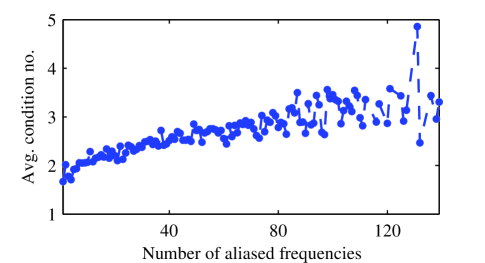
Figure 8: Condition numbers mean value vs. number of aliased frequencies for 4 bands, 200 MHz width real signals, $F_{\textrm{total}}=12$ GHz

The recovery scheme was tested against real-valued signals with $8$ bands ($4$ positive frequencies bands and $4$ negative frequencies bands). The signals without noise were generated and sampled exactly as in the noiseless simulations of real signals. Noise was added randomly at each frequency of the pre-sampled signal according to a normal distribution with standard deviation $\sigma=0.04$; the SNR was defined by $10\log_{10}(1/(\sigma\sqrt{F_{\max}/F^{2}}))=10.5$ dB. This definition takes into account the accumulation of noise in baseband due to sampling. The sampling rates were the same as those in the noiseless simulations. The indicator functions $\chi^{i}[l]$ were constructed using the same parameters as those used in [9]. Each band in $\chi[l]$ was widened by 20 percent on each side. The sub-blocks used in the modified OMP had spectral width of 100 MHz.

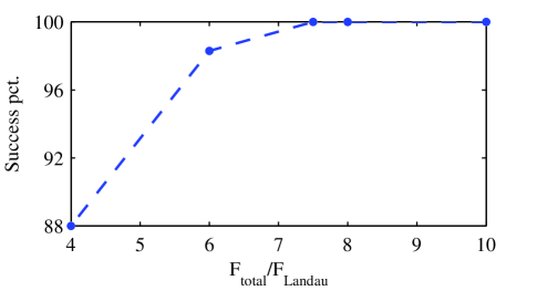
Figure 9: Empirical success percentages for 4 bands of real signals noise that were contaminated with a noise with a standard deviation of $\sigma=0.04$ for different spectral supports of the signal ($F_{\textrm{Landau}}$) with $F_{\textrm{Nyquist}}$=40 GHz, and a total sampling rate $F_{\textrm{total}}=12$ GHz

The success was measured by the algorithm’s ability to achieve a low error $l_{1}$ norm below $2\sigma\sqrt{F_{\max}/F^{2}}=4.47\sigma$ for each recovered band. The mean error for each recovered band $X_{\textrm{rec}}(f)$ and the true band $X(f)$ were evaluated as follows:

$$\frac{1}{|B|}\int_{B}|X_{\textrm{rec}}(f)-X(f)|df<2\sigma\sqrt{F_{\max}/F^{2}}$$

where $B$ is the band support.

Statistics on recovering $8$ bands 200 MHz width each are based on 10000 tests. The simulation showed that, although the algorithm’s performance inevitably decreased, it still achieved a high empirical recovery rate (37 failures out of 10000 tests). Additional simulations were performed by changing the Landau rates as was done in the simulations performed for the noiseless case. In Fig. 9 the empirical success percentage is presented for 1000 simulations of noisy signals. The results of the simulations are similar to those in the noiseless case. When the total sampling rate is 8 times higher than the Landau rate, high success percentage was achieved. The recovery error level depended on the threshold choice. Lower threshold allows more accurate reconstruction but increases the recovery time. Moreover, additional parameters adjustments are also necessary (widening percentage, sub-blocks size). Different error criteria are also possible. For example, choosing $l_{2}$ norm instead of $l_{1}$ norm and setting the error threshold to be $3.3\sigma$ as in [9] resulted in $99.5$ percent empirical success rate in recovering 1.6 GHz Landau rate signals and $99.8$ percent for 1.5 GHz Landau rate signals. This is in contrast to simulations results in Fig. 9 where empirical perfect reconstruction was obtained for those signals under different criteria.

5 Conclusions

In this paper we describe a synchronized multirate sampling scheme for accurately reconstructing sparse multiband signals using a small number of sampling channels (3 in our simulations) whose total sampling rate is significantly lower than the Nyquist rate.

Although the same data that is obtained from our scheme can be obtained by a multicoset scheme, such a multicoset scheme requires many more channels and a time accuracy that cannot be attained practically. Moreover, our scheme processes the data differently, in a way that results in significantly wider basebands and thus greatly reduces the effects of aliasing. By synchronizing the sampling channels our scheme is able to reconstruct signals correctly even in most cases in which the signal is aliased in all the sampling channels.

The main advantage of multicoset sampling schemes is theoretical. Because in a multicoset sampling scheme each channel samples at the same frequency, one has a mathematical structure that enables a perfect reconstructions of ideal multiband signals from samples taken at a total sampling rate that is close to a theoretical lower bound. This bound is attained only under special assumptions regarding the number and width of the signal bands. Moreover, the bound requires the number of sampling channels to be twice the number of signal bands [5]. Hence, in many cases the number of sampling channels becomes too high for a practical implementation.

The main advantage of the SMRS is in the use of a small number of sampling channels that operate at relatively high rates that can reconstruct accurately sparse signal that consist of several bands. Sampling at higher rates has a fundamental advantage in that it increases the SNR after sampling. Another advantage is that implementation of the SMRS scheme does not require a priori knowledge of the maximum width of the signal bands. A third advantage of our scheme is that, in many cases the signal can be reconstructed by simple matrix inversion rather than through a search algorithm as in the multicoset recovery scheme of [5].

In the SMRS scheme, when sampling sparse signals, most of the sampled spectrum is unaliased in at least one of the sampling channels. Hence, most of the spectrum can be reconstructed directly from the unaliased parts of the spectrum. On the other hand, in multicoset sampling schemes an alias in one channel is equivalent to an alias in all channels. Furthermore, a multicoset scheme downconverts signals to much lower frequencies, thus increasing the negative effects of aliasing. Our numerical simulations indicate that the reduced aliasing in our SMRS scheme results in significantly better performance over a multicoset sampling scheme of [5] whose number of sampling channels is small. Also, due to reduced aliasing, it is expected that the reconstruction in the SMRS scheme will be robust when noise is added in the sampling process.

Although we do not have a rigorous criteria for perfect reconstruction, by examining the multicoset pattern that yields the same data it might be possible to obtain necessary conditions for a perfect reconstruction.

Our scheme also solves ill-conditioned linear equations by using a modified OMP algorithm. Whereas we obtained satisfactory results with it, we do not have criteria for determining when the modified OMP algorithm converges to the correct solution. However, this shortcoming may be not as significant because of the possibility of using other algorithms to solve the equations.

6 Appendix

In this appendix we present the modifications to (17) for the real signals recovery. Since the signal is real-valued, its spectrum fulfills

$$X(f)=\overline{X}(-f)$$ (23)

where $\overline{a+bj}=a-bj$ is the complex conjugate and $a$ and $b$ are real numbers.

It follows from (23) and (1), that for each channel index $i$, all the information about $X^{i}(f)$ is contained in the interval $[0,F^{i}/2]$. Consequently, it is convenient to choose the sampling frequencies $F^{i}$ such that $F^{i}/2=\Delta fM^{i}/2$ where $M^{i}/2$ is an integer. Because the conjugation operation $\overline{a+jb}:a+jb\mapsto a-jb$ is not complex linear, (5) needs to be replaced with two systems of equations; one for the real part and one for the imaginary part.

We use the following notations to represent the spectrum of the real signals in the discretized frequencies:

$$X^{i}[k]=X^{i}(k\Delta f)~{}~{}~{}~{}k=-\lfloor M^{i}/2\rfloor,\ldots,\lfloor M^{i}/2\rfloor,$$ (24)

$$X[k]=X(k\Delta f)~{}~{}~{}~{}k=-\lfloor M/2\rfloor,\ldots,\lfloor M/2\rfloor.$$

The sequence $X^{i}[k]$ contains the samples of $X^{i}(f)$ in the baseband $[-F^{i}/2,F^{i}/2]$. The sequence $X[k]$ contains the samples of $X(f)$ given in $[-M\Delta f/2,M\Delta f/2]$, where $M$ is chosen to fulfill $M=\lceil F_{\textrm{Nyquist}}/\Delta f\rceil$. Equation (3) now takes the following form:

$$X^{i}[k]=F^{i}\sum_{l=-\lfloor M/2\rfloor}^{\lfloor M/2\rfloor}X[l]\sum^{\infty}_{n=-\infty}\delta[l-(k+nM^{i})].$$ (25)

Equation (25) can be written in a matrix form as

$$\textbf{x}^{i}=\textbf{A}^{i}\textbf{x}$$ (26)

where $\textbf{x}^{i}$ and x are given by

$$(\textbf{x}^{i})_{k+\lfloor M^{i}/2\rfloor+1} =X^{i}[k],~{}~{}-\lfloor M^{i}/2\rfloor\leq k\leq\lfloor M^{i}/2\rfloor,$$ (27)

$$(\textbf{x})_{k+\lfloor M/2\rfloor+1} =X[k],~{}~{}-\lfloor M/2\rfloor\leq k\leq\lfloor M/2\rfloor,$$

and $\textbf{A}^{i}$ is a matrix whose elements are given by

$$\textbf{A}_{k+\lfloor M^{i}/2\rfloor+1,l+\lfloor M/2\rfloor+1}^{i}=F^{i}\sum^{\infty}_{n=-\infty}\delta[l-(k+nM^{i})].$$ (28)

Note that, since the signal is real valued, all of its spectral information is contained in the positive frequencies.

Each element in $\textbf{A}^{i}$ is equal to either $F^{i}$ or 0. Equation (26) for the different sampling channels can be concatenated as in complex signals case to yield

$$\widehat{\textbf{x}}=\widehat{\textbf{A}}\textbf{x}.$$ (29)

The spectrum can be decomposed into its real and imaginary parts. As a result (29) becomes

$$\widehat{\textbf{x}}^{r}=\widehat{\textbf{A}}^{r}~{}\textbf{x}^{r},$$ (30)

$$\widehat{\textbf{x}}^{im}=\widehat{\textbf{A}}^{im}\textbf{x}^{im}$$

where $\widehat{\textbf{x}}^{r}=\mathrm{Re}(\widehat{\textbf{x}})$ and $\widehat{\textbf{x}}^{im}=\mathrm{Im}(\widehat{\textbf{x}})$. In addition only components that correspond to positive frequencies are retained in the vectors $\widehat{\textbf{x}}^{r}$ and $\widehat{\textbf{x}}^{im}$. The elements of the matrices $\widehat{\textbf{A}}^{r}$ and $\widehat{\textbf{A}}^{im}$ are given by

$$\widehat{\textbf{A}}_{k,\lfloor M/2\rfloor-l+1}^{r}=\widehat{\textbf{A}}_{k,l+1}+\widehat{\textbf{A}}_{k,M-l},~{}~{}l=0,\ldots,\lfloor M/2\rfloor,$$ (31)

$$\widehat{\textbf{A}}_{k,\lfloor M/2\rfloor-l+1}^{im}=\widehat{\textbf{A}}_{k,M-l}-\widehat{\textbf{A}}_{k,l+1},~{}~{}l=0,\ldots,\lfloor M/2\rfloor.$$

The reconstruction is performed with (30) exactly as in the complex case.

References

- [1] H. Landau, ”Necessary density conditions for sampling and interpolation of certain entire functions,” Acta Math., vol. 117, pp. 37-52, July 1967.
- [2] A. Kohlenberg, ”Exact Interpolation of Band-limited Functions,” Appl. Phys., vol. 24,pp. 1432-1436, 1953.
- [3] R. Venkantaramani and Y. Bresler, ”Optimal sub-Nyquist nonuniform sampling and reconstruction for multiband signals,” IEEE Trans. Signal Process., vol. 49, pp. 2301-2313, Oct. 2001.
- [4] Y. M. Lu and M. N. Do, ”A Theory for Sampling Signals from a union of Sub-spaces,” IEEE Trans. Signal Process., to be published.
- [5] M. Mishali and Y. Eldar, ”Blind multiband signal recostruction: compressed sensing for analog signals,” arXiv:0709.1563, Sept. 2007.
- [6] Y. P. Lin and P. P. Vaidyanathan, ”Periodically uniform sampling of bandpass signals,” IEEE Trans. Circuits Sys., vol. 45, pp. 340-351, Mar. 1998.
- [7] C. Herley and W. Wong, ”Minimum rate sampling and reconstruction of signals with arbitrary frequency support,” IEEE Trans. Inform. Theory, vol. 45, pp. 1555-1564, Jul. 1999.
- [8] A.M. Bruckstein, D.L. Donoho and M. Elad, ”From Sparse Solutions of Systems of Equations to Sparse Modeling of Signals and Images,” SIAM, to be published.
- [9] A. Rosenthal, A. Linden and M. Horowitz, ”Multirate asynchronous sampling of multiband signals,” submitted for publication.
- [10] A. Zeitouny, A. Feldser, and M. Horowitz, “Optical sampling of narrowband microwave signals using pulses generated by electroabsorption modulators,” Opt. Comm., vol. 256, pp. 248-255, Dec. 2005.
- [11] I. Stewart and D. Tall, The Foundations of Mathematics, Oxford, England: Oxford University Press, 1977.
- [12] R. Penrose,”A generalized inverse for matrices,” in Proc. Cambridge Philosophical Society, Cambridge, vol. 51, 1955, pp. 406-413.
- [13] R. Venkataramani and Y. Bresler, ”Sampling theorems for uniform and periodic nonuniform MIMO sampling of multiband signals,” IEEE Trans. Signal Process., vol. 51, pp. 3152-3163, Dec. 2003.
- [14] E. J. Cand‘es, J. Romberg and T. Tao, ”Robust uncertainty principles: exact signal reconstruction from highly incomplete frequency information,” IEEE Trans. Inform. Theory, vol. 52, pp. 489-509.