Warm-Chaplygin inflationary universe model

Abstract

Warm inflationary universe models in the context of a Chaplygin gas equation are studied. General conditions required for these models to be realizable are derived and discussed. By using a chaotic potential we develop models for a dissipation coefficient of the form $\Gamma\propto\,\phi^{n}$, with $n=0$ or $n\neq 0$.

I Introduction

It is well know that warm inflation, as opposed to the conventional cool inflation, presents the attractive feature that it avoids the reheating period warm . In these kind of models dissipative effects are important during the inflationary period, so that radiation production occurs concurrently together with the inflationary expansion. If the radiation field is in a highly excited state during inflation, and this has a strong damping effect on the inflaton dynamics, then, it is found a strong regimen of warm inflation. Also, the dissipating effect arises from a friction term which describes the processes of the scalar field dissipating into a thermal bath via its interaction with other fields. Warm inflation shows how thermal fluctuations during inflation may play a dominant role in producing the initial fluctuations necessary for Large-Scale Structure (LSS) formation. In these kind of models the density fluctuations arise from thermal rather than quantum fluctuations 62526 . These fluctuations have their origin in the hot radiation and influence the inflaton through a friction term in the equation of motion of the inflaton scalar field 1126 . Among the most attractive features of these models, warm inflation end at the epoch when the universe stops inflating and ”smoothly” enters in a radiation dominated Big-Bang phasewarm . The matter components of the universe are created by the decay of either the remaining inflationary field or the dominant radiation field taylorberera .

On the other hand, the generalized Chaplygin gas has been proposed as an alternative model for describing the present accelerating of the universe. The generalized Chaplygin gas is described by an exotic equation of state of the form Bento

$$p_{ch}=-\frac{A}{\rho_{ch}^{\beta}},$$ (1)

where $\rho_{ch}$ and $p_{ch}$ are the energy density and pressure of the generalized Chaplygin gas, respectively. $\beta$ is a constant that lies in the range $0<\beta\leq 1$, and $A$ is a positive constant. The original Chaplygin gas corresponds to the case $\beta=1$ 2 . The above equation of state leads to a density evolution in the form Bento

$$\rho_{ch}=\left[A+\frac{B}{a^{3(1+\beta)}}\right]^{\frac{1}{1+\beta}},$$ (2)

where $a$ is the scale factor and $B$ is a positive integration constant.

The Chaplygin gas emerges as a effective fluid of a generalized d-brane in a (d+1, 1) space time, where the action can be written as a generalized Born-Infeld action Bento . These models have been extensively studied in the literature other . The model parameters were constrained using current cosmological observations, such as, CMB CMB and supernova of type Ia (SNIa) SIa .

In the model of Chaplygin inspired inflation usually the scalar field, which drives inflation, is the standard inflaton field, where the energy density given by Eq.(2), can be extrapolate for obtaining a successful inflationary periodIc . Recently, tachyon-Chaplygin inflationary universe model was studied in Ref.SR , and the dynamics of the early universe and the initial conditions for inflation in a model with radiation and a Chaplygin gas was considered in Ref.Monerat:2007ud . The main goal of the present work is to investigate the possible realization of a warm-Chaplygin inspired inflationary model, where the universe is filled with a self-interacting scalar field and a radiation field. We use astronomical data for constraining the parameters appearing in this model. Specifically, the parameters are constrained from the WMAP observationsWMAP3 ; WMAP .

The outline of the paper is a follows. The next section presents a short review of the modified Friedmann equation and the warm-Chaplygin Inflationary phase. Section III deals with the scalar and tensor perturbations. In Section IV it is presented a chaotic potential in the high dissipation approximation. Here, we give explicit expressions for scalar power spectrum and tensor-scalar ratio for our models. Finally, sect.V summarizes our findings. We chose units so that $c=\hbar=1$.

II The modified Friedmann equation and the Warm-Chaplygin Inflationary phase.

We start by writing down the modified Friedmann equation, by using the FRW metric. In particular, we assume that the gravitational dynamics give rise to a modified Friedmann equation of the form

$$H^{2}=\kappa\,[\rho_{ch}+\rho_{\gamma}]=\kappa\left(\left[A+\rho_{\phi}^{(1+\beta)}\right]^{\frac{1}{1+\beta}}\;\;+\rho_{\gamma}\right),$$ (3)

where $\kappa=8\pi G/3=8\pi/3m_{p}^{2}$ (here $m_{p}$ represents the Planck mass), $\rho_{\phi}=\dot{\phi}^{2}/2+V(\phi)$, $V(\phi)=V$ is the scalar potential and $\rho_{\gamma}$ represents the radiation energy density. The modification is realized from an extrapolation of Eq.(2), so that

$$\rho_{ch}=\left[A+\rho_{m}^{(1+\beta)}\right]^{\frac{1}{1+\beta}}\rightarrow\;\left[A+\rho_{\phi}^{(1+\beta)}\right]^{\frac{1}{1+\beta}},$$ (4)

where $\rho_{m}$ corresponds to the matter energy density Ic . The generalized Chaplygin gas model may be viewed as a modification of gravity, as described in Ref.Ber , and for chaotic inflation, in Ref.Ic . Different modifications of gravity have been proposed in the last few years, and there has been a lot of interest in the construction of early universe scenarios in higher-dimensional models motivated by string/M-theory Ran . It is well-known that these modifications can lead to important effects in the early universe. In the following we will take $\beta=1$ for simplicity, which corresponds to the usual Chaplygin gas.

The dynamics of the cosmological model in the warm-Chaplygin inflationary scenario is described by the equations

$$\ddot{\phi}+\,3H\;\dot{\phi}+V_{,\,\phi}=-\Gamma\;\;\dot{\phi},$$ (5)

and

$$\dot{\rho}_{\gamma}+4H\rho_{\gamma}=\Gamma\dot{\phi}^{2}.$$ (6)

Here $\Gamma$ is the dissipation coefficient and it is responsible of the decay of the scalar field into radiation during the inflationary era. $\Gamma$ can be assumed to be a constant or a function of the scalar field $\phi$, or the temperature $T$, or both warm . Here, we will take $\Gamma$ to be a function of $\phi$ only. In the near future we hope to study more realistic models in which $\Gamma$ not only depends on $\phi$ but also on $T$, expression which could be derived from first principles via Quantum Field Theory Moss ; Bastero . On the other hand, $\Gamma$ must satisfy $\Gamma=f(\phi)>0$ by the Second Law of Thermodynamics. Dots mean derivatives with respect to time, and $V_{,\,\phi}=\partial V(\phi)/\partial\phi$.

During the inflationary epoch the energy density associated to the scalar field is of the order of the potential, i.e. $\rho_{\phi}\sim V$, and dominates over the energy density associated to the radiation field, i.e. $\rho_{\phi}>\rho_{\gamma}$. Assuming the set of slow-roll conditions, i.e. $\dot{\phi}^{2}\ll V(\phi)$, and $\ddot{\phi}\ll(3H+\Gamma)\dot{\phi}$ warm , the Friedmann equation (3) reduces to

$$H^{2}\approx\kappa\,\sqrt{A+\rho_{\phi}^{2}}\approx\kappa\,\sqrt{(A+V^{2})},$$ (7)

and Eq. (5) becomes

$$3H\left[\,1+r\;\right]\dot{\phi}\approx-V_{,\,\phi},$$ (8)

where $r$ is the rate defined as

$$r=\frac{\Gamma}{3H}.$$ (9)

For the high (weak) dissipation regimen, we have $r\gg 1$ ($r<1$).

We also consider that during warm inflation the radiation production is quasi-stable, i.e. $\dot{\rho}_{\gamma}\ll 4H\rho_{\gamma}$ and $\dot{\rho}_{\gamma}\ll\Gamma\dot{\phi}^{2}$. From Eq.(6) we obtained that the energy density of the radiation field becomes

$$\rho_{\gamma}=\frac{\Gamma\dot{\phi}^{2}}{4H},$$ (10)

which could be written as $\rho_{\gamma}=\sigma T_{r}^{4}$, where $\sigma$ is the Stefan-Boltzmann constant and $T_{r}$ is the temperature of the thermal bath. By using Eqs.(8), (9) and (10) we get

$$\rho_{\gamma}=\sigma\,T_{r}^{4}=\frac{r}{12\,\kappa\,(1+r)^{2}}\,\frac{V_{,\,\phi}^{2}}{\sqrt{A+V^{2}}}.$$ (11)

Introducing the dimensionless slow-roll parameter $\varepsilon$, we write

$$\varepsilon\equiv-\frac{\dot{H}}{H^{2}}\simeq\frac{1}{6\kappa\,(1+r)}\,\frac{V\,V_{,\,\phi}^{2}}{(A+V^{2})^{3/2}},$$ (12)

and the second slow-roll parameter $\eta$

$$\eta\equiv-\frac{\ddot{H}}{H\dot{H}}\simeq\,\frac{1}{3\kappa\,(1+r)\,\sqrt{A+V^{2}}}\,\left[V_{,\,\phi\phi}+\frac{V_{,\,\phi}^{2}}{V}-\frac{3}{2}\,\frac{V\,V_{,\,\phi}^{2}}{(A+V^{2})}\right],$$ (13)

where $V_{,\,\phi\phi}=\partial^{2}V/\partial\phi^{2}$.

Note that for $r=0$ (or $\Gamma=0$), the parameters $\varepsilon$ and $\eta$ given by Eqs.(12) and (13) reduced to typical expression corresponding to cool inflation where a the Chaplygin gas is consideredIc .

It is possible to find a relation between the energy densities $\rho_{\gamma}$ and $\rho_{\phi}$ by using Eqs.(11) and (12), so that

$$\rho_{\gamma}=\frac{r}{2(1+r)}\,\frac{(A+\rho_{\phi}^{2})}{\rho_{\phi}}\,\,\varepsilon.$$ (14)

Warm inflation takes place when the parameter $\varepsilon$ satisfying the inequality $\varepsilon<1.$ This condition is analogue to the requirement that $\ddot{a}>0$. The condition given above is rewritten in terms of the energy densities $\rho_{\phi}$ and $\rho_{\gamma}$, so that

$$\frac{(A+\rho_{\phi}^{2})}{\rho_{\phi}}>\frac{2(1+r)}{r}\;\rho_{\gamma}.$$ (15)

Also, inflation ends when the universe heats up at a time when $\varepsilon\simeq 1$, which implies

$$\frac{(A+\rho_{\phi}^{2})}{\rho_{\phi}}\simeq\frac{2(1+r)}{r}\;\rho_{\gamma},$$ (16)

and the number of e-folds at the end of inflation is given by

$$N=-3\;\kappa\,\int_{\phi_{*}}^{\phi_{f}}\frac{\sqrt{A+V^{2}}}{V_{,\,\phi}}(1+r)d\phi\,^{\prime}.$$ (17)

In the following, the subscripts $*$ and $f$ are used to denote to the epoch when the cosmological scales exit the horizon and the end of inflation, respectively.

III Perturbations

In this section we will study the scalar and tensor perturbations for our model. Note that in the case of scalar perturbations the scalar and the radiation fields are interacting. Therefore, isocurvature (or entropy) perturbations are generated besides of the adiabatic ones. This occurs because warm inflation can be considered as an inflationary model with two basics fields Jora1 ; Jora . In this context dissipative effects can produce a variety of spectral, ranging between red and blue 62526 ; Jora , and thus producing the running blue to red spectral suggested by WMAP observationsWMAP .

As argued in Refs.warm ; Liddle , the density perturbation could be written as $\delta_{H}=\frac{2}{5}\frac{H}{\dot{\phi}}\,\delta\phi$. From Eqs.(8) and (9), this expression becomes

$$\delta_{H}^{2}=\frac{36\,\kappa^{2}}{25}\left[\frac{(A+V^{2})\,(1+r)^{2}}{V_{\,,\,\phi}^{2}}\right]\,\delta\phi^{2}.$$ (18)

In the case of high dissipation, the dissipation coefficient $\Gamma$ is much greater that the rate expansion $H$ , i.e. $r=\Gamma/3H\gg 1$ and following Taylor and BereraBere2 , we can write

$$(\delta\phi)^{2}\simeq\,\frac{k_{F}\,T_{r}\,}{2\,\pi^{2}},$$ (19)

where the wave-number $k_{F}$ is defined by $k_{F}=\sqrt{\Gamma H/V}=H\,\sqrt{3r}\geq H$, and corresponds to the freeze-out scale at which dissipation damps out to the thermally excited fluctuations. The freeze-out wave-number $k_{F}$ is defined at the point where the inequality $V_{,\,\phi\,\phi}<\Gamma H$, is satisfied Bere2 .

From Eqs. (18) and (19) it follows that

$$\delta^{2}_{H}\approx\;\frac{18\,\sqrt{3}}{25\,\pi^{2}}\,\frac{T_{r}}{V_{\,,\,\phi}^{2}}\,\,(\kappa\,r\,\sqrt{A+V^{2}}\,)^{5/2}\,.$$ (20)

The scalar spectral index $n_{s}$ is given by $n_{s}-1=\frac{d\ln\,\delta^{2}_{H}}{d\ln k}$, where the interval in wave number is related to the number of e-folds by the relation $d\ln k(\phi)=-dN(\phi)$. From Eq.(20), we get

$$n_{s}\approx\,1\,-\,\left[5\widetilde{\varepsilon}-2\widetilde{\eta}-\zeta\right],$$ (21)

where, the parameters $\widetilde{\varepsilon}$, $\widetilde{\eta}$ and $\zeta$, (for $r\gg 1$) are given by

$$\widetilde{\varepsilon}\approx\frac{1}{6\kappa\,r}\,\frac{V\,V_{,\,\phi}^{2}}{(A+V^{2})^{3/2}},\,\;\;\;\;\;\,\,\widetilde{\eta}\approx\,\frac{1}{3\kappa\,r\,\sqrt{A+V^{2}}}\,\left[V_{,\,\phi\phi}+\frac{V_{,\,\phi}^{2}}{V}-\frac{3}{2}\,\frac{V\,V_{,\,\phi}^{2}}{(A+V^{2})}\right],$$ (22)

and

$$\zeta\approx\frac{V_{,\,\phi}^{2}}{\kappa\,r\,\sqrt{A+V^{2}}}\,\left(\frac{V}{(A+V^{2})}-\frac{2}{3V}\right)+\frac{V_{,\,\phi}}{3\kappa\sqrt{A+V^{2}}}\,\frac{r_{,\,\phi}}{r^{2}},$$ (23)

respectively.

One of the interesting features of the observations from WMAP is that it hints at a significant running in the scalar spectral index $dn_{s}/d\ln k=\alpha_{s}$ WMAP . From Eq.(21) we obtain that the running of the scalar spectral index becomes

$$\alpha_{s}\approx\frac{2\,\widetilde{\varepsilon}\,(A+V^{2})}{V\,V_{,\,\phi}}\,[\,5\,\widetilde{\varepsilon}_{,\phi}-2\,\widetilde{\eta}_{,\phi}-\zeta_{,\phi}\,].$$ (24)

In models with only scalar fluctuations the marginalized value for the derivative of the spectral index is approximately $-0.03$ from WMAP five year dataWMAP .

As it was mentioned in Ref.Bha the generation of tensor perturbations during inflation would produce stimulated emission in the thermal background of gravitational wave. This process changes the power spectrum of the tensor modes by an extra temperature dependently factor given by $\coth(k/2T)$. The corresponding spectrum becomes

$$A^{2}_{g}=\frac{16\pi}{m_{p}^{2}}\left(\frac{H}{2\pi}\right)^{2}\,\coth\left[\frac{k}{2T}\right]\simeq\frac{4\,\kappa}{\pi\,m_{p}^{2}}\,(A+V^{2})^{1/2}\coth\left[\frac{k}{2T}\right],$$ (25)

where the spectral index $n_{g}$, results to be given by $n_{g}=\frac{d}{d\,\ln k}\,\ln\left[\frac{A^{2}_{g}}{\coth[k/2T]}\right]=-2\,\varepsilon$. Here, we have used that $A^{2}_{g}\propto\,k^{n_{g}}\,\coth[k/2T]$ as described in Ref.Bha .

For $r\gg 1$ and from expressions (20) and (25) we may write the tensor-scalar ratio as

$$R(k)=\left.\left(\frac{A^{2}_{g}}{P_{\cal R}}\right)\right|_{\,k_{*}}\simeq\left.\frac{m_{p}}{3\,\sqrt{8\,\pi}}\left[\frac{V_{\,,\,\phi}^{2}}{T_{r}\,\,r^{5/2}\,(A+V^{2})^{3/4}}\,\coth\left(\frac{k}{2T}\right)\right]\right|_{\,k=k_{*}}.$$ (26)

Here, $\delta_{H}\equiv\,2\,P_{\cal R}^{1/2}/5$ and $k_{*}$ is referred to $k=Ha$, the value when the universe scale crosses the Hubble horizon during inflation.

Combining WMAP observations WMAP3 ; WMAP with the Sloan Digital Sky Survey (SDSS) large scale structure surveys Teg , it is found an upper bound for $R$ given by $R(k_{*}\simeq$ 0.002 Mpc^-1)$<0.28\,(95\%CL)$, where $k_{*}\simeq$0.002 Mpc^-1 corresponds to $l=\tau_{0}k\simeq 30$, with the distance to the decoupling surface $\tau_{0}$= 14,400 Mpc. The SDSS measures galaxy distributions at red-shifts $a\sim 0.1$ and probes $k$ in the range 0.016 $h$ Mpc^-1$<k<$0.011 $h$ Mpc^-1. The recent WMAP observations results give the values for the scalar curvature spectrum $P_{\cal R}(k_{*})\equiv\,25\delta_{H}^{2}(k_{*})/4\simeq 2.3\times\,10^{-9}$ and the scalar-tensor ratio $R(k_{*})\simeq 0.055<0.2$. We will make use of these values to set constrains on the parameters for our model.

IV Chaotic potential in the high dissipation approach

Let us consider an inflaton scalar field $\phi$ with a chaotic potential. We write for the chaotic potential as $V=m^{2}\phi^{2}/2$, where $m$ is the mass of the scalar field. An estimation of this parameter is given for cool-Chaplygin inflation in Ref.Ic and for warm inflation in Ref.Bere2 . In the following, we develop models for constant and variable dissipation coefficient $\Gamma$, and we will restrict ourselves to the high dissipation regimen, i.e. $r\gg 1$.

IV.1 $\Gamma=const.=\Gamma_{0}$ case.

By using the chaotic potential, we find that from Eq.(8)

$$\dot{\phi}=-\frac{m^{2}\,\phi}{\Gamma_{0}}\Longrightarrow\,\phi(t)=\phi_{0}\,e^{-m^{2}\,t/\Gamma_{0}},$$ (27)

and during the inflationary scenario the scalar field decays due to dissipation into the radiation field. The Hubble parameter is given by

$$H(t)=\sqrt{\kappa}\,\left(A+\frac{m^{4}}{4}\,\phi_{0}^{4}\,e^{-2m^{2}\,t/\Gamma_{0}}\right)^{1/4}.$$ (28)

Note that in the limit $A\longrightarrow 0$ the Hubble parameter coincide with Ref.Bere2 . The dissipation parameter $r$ in this case is

$$r(t)=\frac{\Gamma_{0}}{3\,\kappa^{1/2}}\,\left(A+\frac{m^{4}}{4}\,\phi_{0}^{4}\,e^{-2m^{2}\,t/\Gamma_{0}}\right)^{-1/4},$$

where we observe that it increases when the cosmological time increases.

By using Eq.(14), we can relate the energy density of the radiation field to the energy density of the inflaton field to

$$\rho_{\gamma}=\sqrt{\frac{6}{\pi}}\;\left(\frac{m^{2}\,m_{p}}{8\,\Gamma_{0}}\right)\,\frac{\rho_{\phi}}{(A+\rho_{\phi}^{2})^{1/4}}.$$ (29)

Note again that in the limit $A\longrightarrow 0$, Eq.(29) coincides with that corresponding to the case where the Chaplygin gas is absentBere2 , i.e. $\rho_{\gamma}\propto\rho_{\phi}^{1/2}$.

From Eq.(20), we obtain that the scalar power spectrum becomes

$$P_{\cal R}(k)\approx\left.\;\frac{9\;\sqrt{3}}{4\,\pi^{2}}\,\frac{T_{r}}{m^{2}\,V}\,\;\left[\frac{\kappa^{1/2}\,\Gamma_{0}\,(A+V^{2})^{1/4}}{3}\right]^{5/2}\right|_{\,k=k_{*}},$$ (30)

and from Eq.(26) the tensor-scalar ratio is given by

$$R(k)\approx\;\left.\frac{m_{p}}{3\,\sqrt{2\pi}}\;\left(\frac{3\,\kappa^{1/2}}{\Gamma_{0}}\right)^{5/2}\;\left[\frac{m^{2}\,V}{T_{r}\,(A+V^{2})^{1/8}}\,\;\;\coth\left(\frac{k}{2T}\right)\right]\right|_{\,k=k_{*}}.$$ (31)

By using the WMAP observations where $P_{\cal R}(k_{*})\simeq 2.3\times 10^{-9}$, $R(k_{*})=0.055$, and choosing the parameter $T\simeq\,T_{r}$, we obtained from Eqs.(30) and (31) that

$$V_{*}\simeq\frac{4\times 10^{-5}\,T_{r}}{m^{2}}\,\left[\frac{m_{p}^{2}\,\Gamma_{0}^{2}}{\coth(k_{*}/2T_{r})}\right]^{5/4},$$ (32)

and

$$A=\frac{10^{-21}\,m_{p}^{8}}{\coth^{2}(k_{*}/2T_{r})\,}\,-V_{*}^{2}.$$ (33)

From Eqs.(32) and (33), and since $A>0$, we obtained a lower limit for $m$ given by

$$m^{2}>10^{6}\,T_{r}\;\left[\frac{\Gamma_{0}^{5}}{m_{p}^{3}\,\sqrt{\coth[k_{*}/2T_{r}]}}\right]^{1/2},$$ (34)

and also we find an upper limit for the chaotic potential when the universe scale crosses the Hubble horizon during inflation, given by

$$V_{*}<10^{-11}\,\frac{m_{p}^{4}}{\coth[k_{*}/2T_{r}]}.$$ (35)

Now we consider the special case in which we fixe $T\simeq\,T_{r}\simeq 0.24\times 10^{16}$ GeV and $\Gamma_{0}\simeq 0.5\times 10^{13}$ GeV. In this special case we obtained that the lower limit for the square mass of the scalar field, is given by $m^{2}>4\times 10^{-15}\,m_{p}^{2}$, and for the chaotic potential we obtained an upper limit given by $V_{*}<10^{-14}m_{p}^{4}$.

Figure 1: In this figure we plot the parameter $(m/m_{p})^{2}$ as a function of the dissipation coefficient $\Gamma_{0}/m_{p}$. Here, we have taken the values $T\simeq\,T_{r}\simeq 0.24\times 10^{16}$ GeV and $k_{*}=0.002$ Mpc^-1.

In Fig.(1) we have plotted the parameter $(m/m_{p})^{2}$ versus the dissipation coefficient $\Gamma_{0}/m_{p}$. In doing this, we have used Eqs. (21), (32) and (33). Here, we have taken the values $T\simeq\,T_{r}\simeq 0.24\times 10^{16}$ GeV and $k_{*}=0.002$ Mpc^-1.

IV.2 $\Gamma\propto\,\phi^{n}$ case.

In this case we consider a power-law dissipation coefficient given by

$$\Gamma(\phi)=\alpha_{n}\,\phi^{n},$$ (36)

where $n$ is a positive integer number and $\alpha_{n}$ is a positive constant. The case $n=1$ was studied in Ref.62526 , the case $n=2$ was developed in Ref. Jora1 , and the general case for any $n$ in Ref.Lee:1999iv .

From Eq.(8) we find that

$$\phi(t)=\left[\phi_{i}^{n}-\frac{n\,m^{2}}{\alpha_{n}}\,t\right]^{1/n},$$ (37)

where $\phi(t=0)=\phi_{i}$. The dissipation parameter, $r$, as function of the cosmological time becomes

$$r(t)=\frac{\alpha_{n}}{3\,\kappa^{1/2}}\,\left[\phi_{i}^{n}-\frac{n\,m^{2}}{\alpha_{n}}\,t\right]\,\left[A+\frac{m^{4}}{4}\,\left(\phi_{i}^{n}-\frac{n\,m^{2}}{\alpha_{n}}\,t\right)^{4/n}\right]^{-1/4},$$ (38)

and in the high dissipation approach it is necessary to satisfy that

$$\frac{\alpha_{n}}{3\,\kappa^{1/2}}\,\left[\phi_{i}^{n}-\frac{n\,m^{2}}{\alpha_{n}}\,t\right]\gg\,\,\left[A+\frac{m^{4}}{4}\,\left(\phi_{i}^{n}-\frac{n\,m^{2}}{\alpha_{n}}\,t\right)^{4/n}\right]^{1/4}.$$

Using Eq.(14), we can relate the energy density of the radiation field to the energy density of the inflaton field as

$$\rho_{\gamma}=\sqrt{\frac{6}{\pi}}\;\left(\frac{m^{2+n}\,m_{p}}{8\,2^{n/2}\,\alpha_{n}}\right)\,\frac{\rho_{\phi}^{1-n/2}}{(A+\rho_{\phi}^{2})^{1/4}}.$$ (39)

From Eq.(20), we obtain that the scalar power spectrum becomes

$$P_{\cal R}(k)\approx\left.\;\frac{9\;\sqrt{3}}{4\,\pi^{2}}\,\frac{T_{r}\,V^{\frac{5n-4}{4}}}{m^{\frac{5n+4}{2}}}\,\;\left[\frac{2^{n/2}\,\kappa^{1/2}\,\alpha_{n}\,\,(A+V^{2})^{1/4}}{3}\right]^{5/2}\right|_{\,k=k_{*}},$$ (40)

and from Eq.(26) the tensor-scalar ratio becomes given by

$$R(k)\approx\;\left.\frac{m_{p}}{3\,\sqrt{8\pi}}\;\left(\frac{3\,\kappa^{1/2}}{\alpha_{n}}\right)^{5/2}\;\left[\frac{m^{\frac{4+5n}{2}}\,\,(2\,V)^{\frac{4-5n}{4}}}{T_{r}\,(A+V^{2})^{1/8}}\,\;\;\coth\left(\frac{k}{2T}\right)\right]\right|_{\,k=k_{*}}.$$ (41)

By using the WMAP observations where $P_{\cal R}(k_{*})\simeq 2.3\times 10^{-9}$, $R(k_{*})=0.055$, and choosing the parameter $T\simeq\,T_{r}$, we obtained from Eqs.(40) and (41) that

$$m\approx\left[\frac{3.7\times 10^{-4}}{a^{1/4}\,b^{5/4}\,V_{*}^{\frac{4-5n}{4}}}\right]^{\frac{2}{4+5n}},$$ (42)

and

$$A\approx\,5.9\times 10^{-11}\,\left[\frac{8.1\times 10^{-10}}{a^{2}\,b^{2}}-1.7\times 10^{10}\,V_{*}^{2}\right],$$ (43)

where $a$ and $b$ are given by

$$a=\frac{2^{\frac{5n-8}{4}}\,T_{r}\,\kappa^{5/4}\,\alpha_{n}^{5/2}}{\pi^{2}},\;\;\;\mbox{and}\;\;\;\;b=\frac{m_{p}\,3^{3/2}}{\sqrt{\pi}\,\,2^{\frac{2+5n}{4}}}\;\frac{\kappa^{5/4}}{\alpha_{n}^{5/2}\;T_{r}}\,\coth\left(\frac{k_{*}}{2\,T_{r}}\right),$$

respectively.

Using that $A>0$, then we find from Eqs. (42) and (43) a lower limit for the mass of the inflaton $m$, independent of the value $V_{*}$, and it becomes

$$m\,>\,\left[\frac{a^{3-5n}\;10^{\frac{44-95n}{2}}}{b^{1+5n}}\right]^{\frac{1}{2(4+5n)}}.$$ (44)

For instance, for $n=1$ we obtained from Eq.(44), that $m>10^{-1}\,[T_{r}^{2}\,\alpha_{n=1}^{5}/\kappa^{5}]^{1/9}\,[m_{p}\,\coth(k_{*}/2T_{r})]^{-1/3}$$\sim 7\times 10^{-7}m_{p}$. Here, we have used that $T_{r}\simeq 10^{-3}m_{p}$, $k_{*}=0.002$Mpc^-1 and $\alpha_{n=1}\simeq 10^{-5}$ (see Ref.62526 ). Note that this lower limit for $m$ decreases when the parameter $\alpha_{n=1}$ decreases. For $n>1$ we noted that a similar situation occurs for the lower limit of $m$, i.e., this limit decreases when the parameter $\alpha_{n}$ decreases. In Fig.2 we have plotted the running spectral index $\alpha_{s}$ versus the scalar spectrum index $n_{s}$, for a dissipation coefficient $\Gamma(\phi)=\alpha_{n=1}\,\phi$. In doing this, we have taken two different values for the parameter $\alpha_{n=1}$ and choosing the parameters $T\simeq T_{r}\simeq 0.24\times 10^{16}$GeV and $k_{*}=0.002$Mpc^-1. Note that for $\alpha_{n=1}\sim 10^{-5}-10^{-7}$ and for a given $n_{s}\sim 0.95$ the values of $\alpha_{s}$ becomes in agrement with that registered by the WMAP observations. From Fig. 3 we note that the parameter $A\sim 10^{-25}m_{p}^{8}$ becomes smaller by one order of magnitude when it is compared with the case of Chaplygin cool-inflation Ic , and smaller by two order of magnitude when it is compared with the case of tachyon-Chaplygin inflationary universe model SR .

Another interesting situation corresponds to the case when $\Gamma=\alpha_{n=2}\,\phi^{2}$. Following a similar approach to those of the previous cases, we obtained that $\alpha_{n=2}\sim 10^{-13}/m_{p}-10^{-5}/m_{p}$ and $A\sim 10^{-26}m_{p}^{8}$ in order to be in agrement with WMAP five year dataWMAP . Note that this value of $A$ is similar to those found for the case $n=1$. Here, again we have taken the parameters $T\simeq T_{r}\simeq 0.24\times 10^{16}$GeV, $k_{*}=0.002$Mpc^-1 and $n_{s}\simeq 0.95$.

In Fig.4 we show the plot of the adimensional parameter $\alpha_{n}/m_{p}^{1-n}$ in terms of the parameters $n$ on the one hand, and $m/m_{p}$ in addition. In doing this, we have used Eqs. (21), (24), (42) and (43). Here, we have used the WMAP five year data, and we have taken three different values for the parameters $n$ and $m/m_{p}$. Also, we have chosen $T\simeq T_{r}\simeq 0.24\times 10^{16}$GeV and $k_{*}=0.002$Mpc^-1, as above.

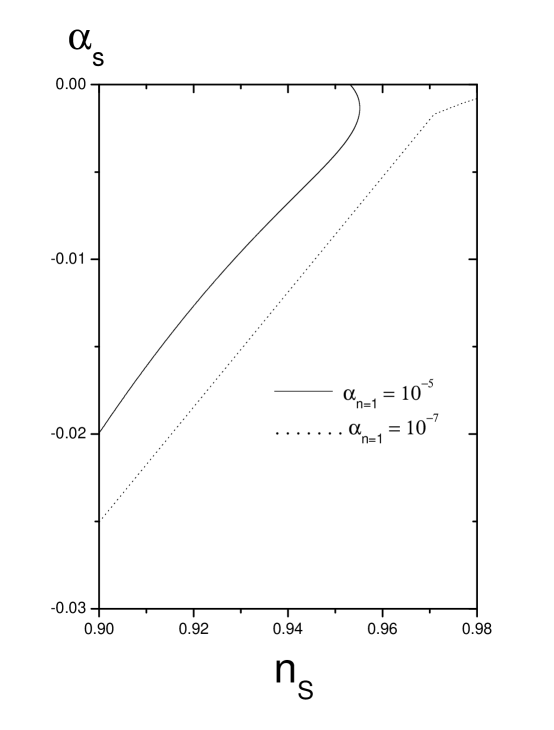
Figure 2: Evolution of the running scalar spectral index $\alpha_{s}$ versus the scalar spectrum index $n_{s}$ in the model $\Gamma\propto\,\phi$, for two different values of the parameter $\alpha_{n=1}$.

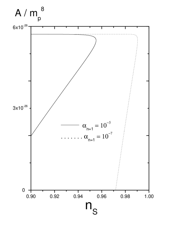
Figure 3: The parameter $A$ versus the scalar spectrum index $n_{s}$ in the model $\Gamma\propto\,\phi$, for two different values of the parameter $\alpha_{n=1}$.

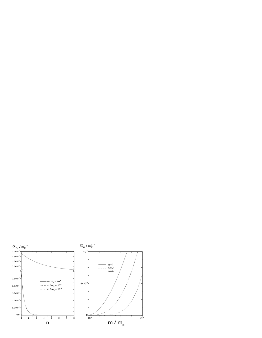
Figure 4: The left panel shows the parameter $\alpha_{n}/m_{p}^{1-n}$ as a function of the parameter $n$. The right panel shows the parameter $\alpha_{n}/m_{p}^{1-n}$ versus the mass of the inflaton field $m/m_{p}$. In both cases, we have taken the parameters $T\simeq T_{r}\simeq 0.24\times 10^{16}$GeV and $k_{*}=0.002$Mpc^-1.

V Conclusions

In this paper we have investigated the warm-Chaplygin inflationary scenario. In the slow-roll approximation we have found a general relationship between the radiation and scalar field energy densities. This has led us to a general criterium for warm-Chaplygin inflation to occur.

Our specific models are described by a chaotic potential and we have consider different cases for the dissipation coefficient, $\Gamma$. In the first case, we took $\Gamma=constant=\Gamma_{0}$. Here, we have found solutions for the inflaton field and the Hubble parameter. The relation between the radiation field and the inflaton field energy densities presents the same characteristic to that corresponding to the warm inflation case, except that it depends on the extra parameter $A$. For the case in which the dissipation coefficient $\Gamma$ is taken to be a function of the scalar field, i.e. $\Gamma\propto\phi^{n}$, it was possible to describe an appropriate warm inflationary universe model for $n=1$ and $n=2$. In these cases, we have obtained explicit expressions for the corresponding scalar spectrum and the running of the scalar spectrum indices.

Finally, by using the WMAP five year dataWMAP and for the special case where $T\simeq T_{r}\simeq 0.24\times 10^{16}$GeV, $k_{*}=0.002$Mpc^-1 and $n_{s}\simeq 0.95$, we have found new constraints on the parameters $\alpha_{n}$, $A$ and $m$.

- (1) A. Berera, Phys. Rev. Lett. 75, 3218 (1995); A. Berera, Phys. Rev. D 55, 3346 (1997).
- (2) L.M.H. Hall, I.G. Moss and A. Berera, Phys.Rev.D 69, 083525 (2004); I.G. Moss, Phys.Lett.B 154, 120 (1985); A. Berera and L.Z. Fang, Phys.Rev.Lett. 74 1912 (1995); A. Berera, Nucl.Phys B 585, 666 (2000).
- (3) A. Berera, Phys. Rev.D 54, 2519 (1996).
- (4) A. Berera, Phys. Rev. D 55, 3346 (1997); J. Mimoso, A. Nunes and D. Pavon, Phys.Rev.D 73, 023502 (2006); R. Herrera, S. del Campo and C. Campuzano, JCAP 10, 009 (2006); S. del Campo, R. Herrera and D. Pavon, Phys. Rev. D 75, 083518 (2007); S. del Campo and R. Herrera, Phys. Lett. B 653, 122 (2007); M. A. Cid, S. del Campo and R. Herrera, JCAP 10, 005 (2007); J. C. B. Sanchez, M. Bastero-Gil, A. Berera and K. Dimopoulos, arXiv:0802.4354 [hep-ph].
- (5) M. C. Bento, O. Bertolami and A. Sen, Phys. Rev. D 66, 043507 (2002).
- (6) A. Kamenshchik, U. Moschella and V. Pasquier, Phys. Lett. B 511, 265 (2001).
- (7) H. B. Benaoum, arXiv:hep-th/0205140; A. Dev, J.S. Alcaniz and D. Jain, Phys. Rev. D 67 023515 (2003); G. M. Kremer, Gen. Rel. Grav. 35, 1459 (2003); R. Bean, O. Dore, Phys. Rev. D 68, 023515 (2003); Z.H. Zhu, Astron. Astrophys. 423, 421 (2004); H. Sandvik, M. Tegmark, M. Zaldarriaga and I. Waga, Phys. Rev. D 69, 123524 (2004) ; L. Amendola, I. Waga and F. Finelli, JCAP 0511, 009 (2005); P.F. Gonzalez-Diaz, Phys. Lett. B 562, 1 (2003) ; L.P. Chimento, Phys. Rev. D 69, 123517 (2004); L.P. Chimento and R. Lazkoz, Phys. Lett. B 615, 146 (2005); U. Debnath, A. Banerjee and S. Chakraborty, Class. Quant. Grav. 21, 5609 (2004); W. Zimdahl and J.C. Fabris, Class. Quant. Grav. 22, 4311 (2005); P. Wu and H. Yu,Class. Quant. Grav. 24, 4661 (2007); M. R. Setare, Phys. Lett. B 654, 1 (2007); M. Bouhmadi-Lopez and R. Lazkoz, Phys. Lett. B 654, 51 (2007).
- (8) M.C. Bento, O. Bertolami and A. Sen, Phys. Lett. B 575, 172 (2003); M.C. Bento, O. Bertolami and A.A. Sen, Phys. Rev. D67, 063003 (2003).
- (9) M. Makler, S.Q. de Oliveira and I. Waga, Phys. Lett. B 555, 1 (2003); J.C. Fabris, S.V.B. Goncalves and P.E. de Souza, arXiv:astro-ph/0207430; M. Biesiada, W. Godlowski and M. Szydlowski, Astrophys. J. 622, 28 (2005); Y. Gong and C.K. Duan, Mon. Not. Roy. Astron. Soc. 352, 847 (2004); Y. Gong, JCAP 0503, 007 (2005) .
- (10) O. Bertolami and V. Duvvuri, Phys. Lett. B 640, 121 (2006).
- (11) S. del Campo and R. Herrera, Phys. Lett. B 660, 282 (2008).
- (12) G. A. Monerat et al., Phys. Rev. D 76, 024017 (2007).
- (13) D. N. Spergel et al. [WMAP Collaboration], Astrophys. J. Suppl. 170, 377 (2007).
- (14) J. Dunkley et al. [WMAP Collaboration], arXiv:0803.0586 [astro-ph]; G. Hinshaw et al., arXiv:0803.0732 [astro-ph].
- (15) T. Barreiro, A.A. Sen, Phys. Rev. D 70, 124013 (2004).
- (16) L. Randall and R. Sundrum, Phys. Rev. Lett. 83, 4690 (1999); T. Shiromizu, K. Maeda and M. Sasaki, Phys. Rev. D 62, 024012 (2000); D. Dvali, G. Gabadadze and M. Porrati, Phys.Lett. B 485, 208 (2000); K. Freese and M. Lewis, Phys. Lett. B 540, 1 (2002); R. Maartens, Lect. Notes Phys. 653 213 (2004); A. Lue, Phys. Rept. 423, 1 (2006).
- (17) I.G.Moss and C. Xiong, hep-ph/0603266.
- (18) M. Bastero-Gil and A. Berera, Phys. Rev. D 76, 043515 (2007).
- (19) A. Starobinsky and J. Yokoyama, Density fluctuations in Brans-Dicke inflation, Published in the Proceedings of the Fourth Workshop on General Relativity and Gravitation. Edited by K. Nakao, et al. Kyoto, Kyoto University, 1995. pp. 381, gr-qc/9502002; A. Starobinsky and S. Tsujikawa, Nucl.Phys.B 610, 383 (2001);
- (20) H. Oliveira, Phys. Lett. B 526, 1 (2002); H. Oliveira and S. Joras, Phys. Rev. D 64, 063513 (2001).
- (21) A. Liddle and D. Lyth, Cosmological inflation and large-scale structure, 2000, Cambridge University;J. Linsey , A. Liddle, E. Kolb and E. Copeland, Rev. Mod. Phys 69, 373 (1997); B. Bassett, S. Tsujikawa and D. Wands, Rev. Mod. Phys. 78, 537 (2005).
- (22) A. Taylor and A. Berera, Phys. Rev. D 69, 083517 (2000).
- (23) K. Bhattacharya, S. Mohanty and A. Nautiyal, Phys.Rev.Lett. 97, 251301 (2006).
- (24) M. Tegmark et al., Phys. Rev. D 69, 103501 (2004).
- (25) W. Lee and L. Z. Fang, Phys. Rev. D 59, 083503 (1999)