Mass distribution and orbital anisotropy of early-type galaxies: constraints from the Mass Plane

Abstract

Massive early-type galaxies are observed to lie on the Mass Plane (MP), a two-dimensional manifold in the space of effective radius $R_{\rm e}$, projected mass $M_{\rm e2}^{\rm p}$ (measured via strong gravitational lensing) and projected stellar velocity dispersion $\sigma_{\rm e2}$ within $R_{\rm e}/2$. The MP is less ‘tilted’ than the traditional Fundamental Plane, and the two have comparable associated scatter. This means that the dimensionless structure parameter $c_{\rm e2}=2GM_{\rm e2}^{\rm p}/(R_{\rm e}\sigma_{\rm e2}^{2})$ is a nearly universal constant in the range $\sigma_{\rm e2}=175-400$ km s^-1. This finding can be used to constrain the mass distribution and internal dynamics of early-type galaxies: in particular, we explore the dependence of $c_{\rm e2}$ on light profile, dark-matter distribution, and orbital anisotropy for several families of spherical galaxy models. We find that a relatively wide class of models has values of $c_{\rm e2}$ in the observed range, because $c_{\rm e2}$ is not very strongly sensitive to the mass distribution and orbital anisotropy. The degree of fine tuning required to match the small intrinsic scatter of $c_{\rm e2}$ depends on the considered family of models: if the total mass distribution is isothermal ($\propto r^{-2}$), a broad range of stellar luminosity profile and anisotropy is consistent with the observations, while Navarro, Frenk & White dark-matter halos require more fine tuning of the stellar mass fraction, luminosity profile and anisotropy. If future data can cover a broader range of masses, the MP could be seen to be tilted by the known non-homology of the luminosity profiles of early-type galaxies, and the value of any such tilt would provide a discriminant between models for the total mass-density profile of the galaxies.

1 Introduction

The origin of empirical scaling laws is a key open issue in observational cosmology. Galaxies do not come in all sizes, shapes, colours, but rather tend to to live in lower-dimensional manifolds, which represent a stringent testing ground for theories of galaxy formation and evolution.

Early-type galaxies obey a particularly tight scaling law: the so-called Fundamental Plane (FP; Djorgovsky & Davis, 1987; Dressler et al., 1987). In the space of effective radius $R_{\rm e}$, central velocity dispersion $\sigma_{\rm e8}$ and effective surface brightness $\langle I\rangle_{\rm e}{\equiv}L/(2\pi R_{\rm e}^{2})$ (where $L$ is the total luminosity of the galaxy), they lie on the following relation with remarkably small scatter (${\,\mathrel{\mathchoice{\lower 2.9pt\vbox{\halign{$\m@th\displaystyle\hfil#\hfil$\cr<\crcr\sim\crcr}}}{\lower 2.9pt\vbox{\halign{$\m@th\textstyle\hfil#\hfil$\cr<\crcr\sim\crcr}}}{\lower 2.9pt\vbox{\halign{$\m@th\scriptstyle\hfil#\hfil$\cr<\crcr\sim\crcr}}}{\lower 2.9pt\vbox{\halign{$\m@th\scriptscriptstyle\hfil#\hfil$\cr<\crcr\sim\crcr}}}\,}}20\%$ in $R_{\rm e}$; Bernardi et al., 2003b):

$$\log R_{\rm e}=a\log\sigma_{\rm e8}+b\log\langle I\rangle_{\rm e}+\mathit{const},$$ (1)

where the numerical value of $a$ and $b$ depends somewhat upon the wavelength of observations and upon the sample and the fitting method (Pahre, Djorgovski & de Carvalho, 1998; Bernardi et al., 2003b). The FP is said to be ‘tilted’, in the sense that the coefficients $a$ and $b$ differ significantly from the values $a=2$ and $b=-1$ expected for structurally and dynamically homologous systems with luminosity-independent stellar mass-to-light ratio and dark-matter distribution. Several explanations have been proposed for the tilt, including a systematic dependence of stellar mass-to-light ratio or dark-matter content and distribution upon luminosity (and hence presumably upon mass), structural non-homology and orbital anisotropy (e.g. Faber et al., 1987; Bender, Burstein & Faber, 1992; Renzini & Ciotti, 1993; Ciotti, Lanzoni & Renzini, 1996; Borriello, Salucci & Danese, 2003).

Recently, Bolton et al. (2007, 2008b), using a sample of strong gravitational lenses, have shown that early-type galaxies lie on a Mass Plane (MP)

$$\log R_{\rm e}=a_{\rm m}\log\sigma_{\rm e2}+b_{\rm m}\log\Sigma_{\rm e2}+\mathit{const},$$ (2)

where $\sigma_{\rm e2}$ is the projected velocity dispersion within an aperture radius $R_{\rm e}/2$ and $\Sigma_{\rm e2}$ is the surface mass density within $R_{\rm e}/2$, with $a_{\rm m}=1.82\pm 0.19$, $b_{\rm m}=-1.20\pm 0.12$ and RMS orthogonal scatter of 1.24 when normalized by the observational errors. The fact that $(a_{\rm m},b_{\rm m})$ are close to $(2,-1)$ and that the scatter is small can be expressed in terms of structural and dynamical homology of the lenses, by defining the dimensionless structure parameter

$$c_{\rm e2}\equiv{2GM_{\rm e2}^{\rm p}\over R_{\rm e}\sigma_{\rm e2}^{2}},$$ (3)

where $M_{\rm e2}^{\rm p}$ is the total projected mass within $R_{\rm e}/2$. For their sample of lens early-type galaxies from the Sloan Lens ACS (SLACS) Survey Bolton et al. (2008b) find on average

$$\langle\log c_{\rm e2}\rangle=0.53\pm 0.057,$$ (4)

which throughout the paper we will refer to as the “observed range” of $c_{\rm e2}$. We note that the observed scatter on $\langle\log c_{\rm e2}\rangle$ is 0.08, but here we consider the estimated intrinsic scatter 0.057 (see Bolton et al., 2008b).

As discussed in several papers (Bolton et al., 2006; Treu et al., 2006; Bolton et al., 2008a; Treu et al., 2008) the SLACS lenses are found to be indistinguishable from control samples of Sloan Digital Sky Survey (SDSS) galaxies with the same stellar velocity dispersion and size, in terms of luminosity/surface brightness, location on the FP, and environment. This inspires some confidence that the results found for the lens sample, including the MP, are generic properties of the overall class of early-type galaxies.

Independent of its origin and theoretical interpretation, the existence of the MP is a powerful empirical tool to estimate galaxy mass by using information on size and velocity dispersion only (Bolton et al., 2007). In addition, it is clear that the very existence of the MP may be used to improve our understanding of galaxy formation and evolution. What is the origin of such a strong correlation among measurable galaxy quantities? Or, in other words, what kinds of galaxy models can be ruled out by the existence of a tight MP? Although this question has been asked before in regards to the traditional FP, the MP provides an additional powerful tool. In fact, there are a few differences between the FP (equation 1) and the MP (equation 2):

1. The FP is sensitive to the galaxy stellar mass-to-light ratio, while the MP is not. This implies that, e.g., the role of stellar populations in establishing the tilt and scatter of the FP can be disentangled by looking at the MP.

2. The FP is traditionally based on the central velocity dispersion $\sigma_{\rm e8}$ (measured within $R_{\rm e}/8$), while the MP has been constructed using $\sigma_{\rm e2}$, which is measured within $R_{\rm e}/2$. This is a consequence of the fixed spatial observing aperture of the SDSS spectrograph; an MP based upon $\sigma_{\rm e8}$ could be constructed using spatially resolved spectroscopy of the SLACS lens sample.

3. The FP combines quantities evaluated on different scales ($R_{\rm e}$, $R_{\rm e}/8$), while MP combines quantities evaluated within the same radius $R_{\rm e}/2$. Again, this is partially due to the fixed SDSS spectroscopic aperture, though the apertures of the lensing mass measurements are fixed by the cosmic configuration of the individual strong-lens systems.

Each of the points above can contribute to make the MP less tilted (and presumably with less scatter) than the FP. For example, given the relatively large spectroscopic aperture used to define $c_{\rm e2}$, we expect it to be robust with respect to changes in the detailed properties of galaxy structure, internal dynamics, and dark-matter content. Similarly, by replacing surface brightness with surface mass density we expect that tilt and scatter due to diversity of chemical composition or star formation history be reduced in MP. Furthermore, having all but removed the effects of stellar population the MP is potentially a cleaner diagnostic than the FP of the structural and dynamical properties of early-type galaxies.

In this paper, we exploit the existence of the MP to constrain important properties of early-type galaxies, such as orbital anisotropy and dark-matter distribution. We achieve this goal by constructing observationally and cosmologically motivated families of galaxy models and finding the range of parameter spaces consistent with the observed range of $c_{\rm e2}$. For the sake of simplicity, in the present investigation we limit ourselves to spherically symmetric models. As with the FP (Faber et al., 1987; Saglia, Bender & Dressler, 1993; Prugniel & Simien, 1994; Lanzoni & Ciotti, 2003; Riciputi et al., 2005), deviation from spherical symmetry is expected to increase the scatter of the MP because of projection effects. Thus, a natural follow-up of the present work would be the extension to non-spherical models.

The paper is organized as follows. In Section 2 we describe the models, in Sections 3 and 4 we present our results, and in Section 5 we conclude.

2 Models

2.1 Methodology and general properties

We consider spherical galaxy models with stellar density distribution $\rho_{*}(r)$ and total density distribution $\rho_{\rm tot}(r)$. The radial component $\sigma_{r}(r)$ of the velocity dispersion tensor is given by solving the Jeans equation (e.g. Binney & Tremaine, 2008)

$${d\rho_{*}\sigma_{r}^{2}\over dr}+{2\beta\rho_{*}\sigma_{r}^{2}\over r}=-\rho_{*}g_{r},$$ (5)

where $g_{r}(r)=d\Phi(r)/dr$, $\Phi(r)$ is the total gravitational potential generated by $\rho_{\rm tot}(r)$, and

$$\beta(r)\equiv 1-{\sigma_{\vartheta}^{2}+\sigma_{\varphi}^{2}\over 2\sigma_{r}^{2}}$$ (6)

is the anisotropy parameter ($\sigma_{\vartheta}$ and $\sigma_{\varphi}$ are, respectively, the $\vartheta$ and $\varphi$ components of the velocity-dispersion tensor).

The line-of-sight velocity dispersion is (Binney & Mamon, 1982)

$$\sigma_{\rm p}^{2}(R)={2\over\Sigma_{*}(R)}\int_{R}^{\infty}\left[{1-\beta(r){R^{2}\over r^{2}}}\right]{\rho_{*}(r)\sigma_{r}^{2}rdr\over\sqrt{r^{2}-R^{2}}},$$ (7)

where

$$\Sigma_{*}(R)=2\int_{R}^{\infty}{\rho_{*}(r)rdr\over\sqrt{r^{2}-R^{2}}}$$ (8)

is the stellar surface density (we assume that the stellar mass-to-light ratio is independent of radius). The aperture velocity dispersion within a projected radius $R$, the closest analog to the measured stellar velocity dispersion, is determined via

$$\sigma_{\rm a}^{2}(R)={2\pi\over M_{\rm*}^{\rm p}(R)}\int_{0}^{R}\Sigma_{*}(R^{\prime})\sigma_{\rm p}^{2}(R^{\prime})R^{\prime}\,dR^{\prime},$$ (9)

where

$$M_{\rm*}^{\rm p}(R)=2\pi\int_{0}^{R}\Sigma_{*}(R^{\prime})R^{\prime}\,dR^{\prime}$$ (10)

is the projected stellar mass within $R$. So, $\sigma_{\rm e8}^{2}\equiv\sigma_{\rm a}^{2}(R_{\rm e}/8)$ and $\sigma_{\rm e2}^{2}\equiv\sigma_{\rm a}^{2}(R_{\rm e}/2)$. Note that the mass weighting expressed here is equivalent to luminosity weighting for the case of a spatially uniform stellar mass-to-light ratio.

Gravitational lensing analysis allows one to measure the total projected mass density within the Einstein radius. The total projected mass within a radius $R$ of a spherical system is

$$M_{\rm tot}^{\rm p}(R)=2\pi\int_{0}^{R}\Sigma_{\rm tot}(R^{\prime})R^{\prime}\,dR^{\prime},$$ (11)

where

$$\Sigma_{\rm tot}(R)=2\int_{R}^{\infty}{\rho_{\rm tot}(r)rdr\over\sqrt{r^{2}-R^{2}}}$$ (12)

is the total surface density. The mass within the Einstein radius, measured by gravitational lensing is obtained by setting $R$ equal to the Einstein radius. The size of the Einstein radius depends on the geometry of the lensing system, through the angular diameter distances between the observer, lens and background source, as well as on the mass distribution of the lens. Typically, for galaxy-size lenses, Einstein radii are of order of one arcsecond, or $\sim$5 kpc for lenses at moderate redshift. For the SLACS lens sample, the Einstein radii are typically about half the effective radius of the lens galaxy.

For a given projected radius $R$ we define the structure parameter

$$c(R)\equiv{GM_{\rm tot}^{\rm p}(R)\over R\sigma_{\rm a}^{2}(R)}.$$ (13)

So, by definition (equation 3) $c_{\rm e2}=c(R_{\rm e}/2)$, because $M_{\rm e2}^{\rm p}\equiv M_{\rm tot}^{\rm p}(R_{\rm e}/2)$.

2.2 Stellar density distribution

We consider two families of stellar density distributions—$\gamma$ models and Sérsic models—that are known to match well the observed surface brightness profiles of early-type galaxies over the range of interest $\sim$1-10 kpc for constant stellar mass-to-light ratios. The density profile of the $\gamma$-models (Dehnen, 1993; Tremaine et al., 1994) is given by

$$\rho_{*}(r)={3-\gamma\over 4\pi}{M_{*}r_{*}\over r^{\gamma}(r_{*}+r)^{4-\gamma}}\qquad(0\leq\gamma<3),$$ (14)

where $M_{*}$ is the total stellar mass. The cases $\gamma=1$ and $\gamma=2$ are the Hernquist (1990) and Jaffe (1983) models, respectively.

In the case of the Sérsic models, the projected density distribution follows the Sérsic (1968) $R^{1/m}$ law:

$$\Sigma_{*}(R)=\Sigma_{*,0}\,\exp\left[-b(m)\left(\frac{R}{R_{\rm e}}\right)^{1/m}\right]$$ (15)

where $b(m)\sim 2m-1/3+4/(405m)$ (Ciotti & Bertin, 1999). For $m=4$ the de Vaucouleurs’ (1948) $R^{1/4}$ law is obtained. By deprojecting $\Sigma_{*}$ one obtains the corresponding intrinsic density distribution (Binney & Tremaine, 2008)

$$\rho_{*}(r)=-{1\over\pi}\int_{r}^{\infty}{d\Sigma_{*}\over dR}{dR\over\sqrt{R^{2}-r^{2}}}.$$ (16)

2.3 Total density distribution

Figure 1: The ratio $\xi=r_{\rm s}/R_{\rm e}$ as a function of the effective radius $R_{\rm e}$ according to equation (24) for NFW plus stars and adiabatically contracted NFW plus stars models (see text for details).

Figure 2: Total (solid lines), stellar (dotted lines), and dark-matter (dashed lines) projected mass distributions $M^{\rm p}(R)$ for $m=4$ Sérsic models with non-contracted (top) and adiabatically contracted (bottom) NFW dark-matter halos of given $\xi=r_{\rm s}/R_{\rm e}$ and stellar-to-total mass fraction $f_{*}$. The projected mass $M^{\rm p}(R)$ is in units of $M_{*}+M_{\rm dm}$. All models have concentration $C_{200}=8$.

We consider four different models for the total density distribution. First we consider a singular isothermal sphere (SIS) model, which provides a generally good description of the lensing properties of early-type galaxies (e.g. Kochanek, 1994; Treu & Koopmans, 2004; Koopmans et al., 2006), as well as of their stellar kinematics (e.g. Bertin et al., 1994; Gerhard et al., 2001). Second, we consider light-traces-mass (LTM) models. Although they are known to fail observational constraints based on statistical analyses of strong lenses (e.g., Rusin et al., 2003; Rusin & Kochanek, 2005; Bolton et al., 2008b), stellar dynamics (e.g., Gerhard et al., 2001), individual strong-lens modeling (e.g., Wayth et al., 2005; Dye & Warren, 2005; Dye et al., 2007; Gavazzi et al., 2008), weak-lensing analysis (e.g., Gavazzi et al., 2007), and combined strong-lens/dynamical analyses (e.g., Koopmans & Treu, 2002, 2003; Treu & Koopmans, 2002, 2003, 2004; Koopmans et al., 2006), they serve as a useful “straw man” hypothesis to test against the MP. Lastly, we consider two families of cosmologically motivated models based on Navarro, Frenk & White (1996, NFW) halos with the addition of stars. In one case (NFW plus stars models, hereafter NFW+S) the stars are added leaving the halo unperturbed; in the other one (adiabatically contracted NFW plus stars models, hereafter acNFW+S), the halo is assumed to “respond” to the sinking of baryons towards the centre of the galaxy as prescribed by the adiabatic contraction recipe of Blumenthal et al. (1986). Several arguments suggest that the Blumenthal et al. (1986) model might overestimate the compression of the halo (see Gnedin et al., 2004; El-Zant et al., 2004; Nipoti et al., 2004). In particular, Gnedin et al. (2004) argued that the standard adiabatic contraction model of Blumenthal et al. (1986), based on some simplifying assumptions such as spherical symmetry and circularity of the particle orbits, tends to overpredict the increase of dark matter density in the central regions. However, considering both NFW+S and acNFW+S we should bracket the realistic range of NFW halo models (see also Jiang & Kochanek, 2007).

We now define for each model the total (stellar plus dark matter) density profile $\rho_{\rm tot}(r)$. As we limit to spherically symmetric distributions, in all cases the modulus of the gravitational field is

$${g_{r}(r)}={GM_{\rm tot}(r)\over r^{2}},$$ (17)

where $M_{\rm tot}(r)=4\pi\int_{0}^{r}\rho_{\rm tot}(r^{\prime})r^{\prime 2}dr^{\prime}$ the total mass within $r$.

In the case of SIS models, the total (stars plus dark matter) density profile is

$$\rho_{\rm tot}(r)={\sigma_{SIS}^{2}\over 2\pi Gr^{2}},$$ (18)

where $\sigma_{SIS}$ is the one-dimensional velocity dispersion of isotropic SIS. For LTM models the total density profile is $\rho_{\rm tot}(r)=K\rho_{*}(r)$, where $K$ is a dimensionless constant (note that $c_{\rm e2}$ is independent of $K$). In NFW+S models the dark-matter halo is described by a NFW model, so the dark-matter density distribution is

$$\rho_{\rm dm}(r)={M_{\rm dm}\over 4\pi f(C_{200})}{1\over r(r+r_{\rm s})^{2}},$$ (19)

where $r_{\rm s}$ is the scale radius, and the distribution is truncated at the virial radius $r_{\rm vir}$. The average dark-matter density within $r_{\rm vir}$ equals 200 times the critical density of the Universe. In the equation above, $C_{200}\equiv r_{\rm vir}/r_{\rm s}$ is the concentration parameter,

$$f(C_{200})=\ln(1+C_{200})-{C_{200}\over 1+C_{200}},$$ (20)

and $M_{\rm dm}$ is the total dark-matter mass. In this case the total (stars plus dark matter) density profile is

$$\rho_{\rm tot}(r)=\rho_{\rm dm}(r)+\rho_{*}(r).$$ (21)

Formally, these NFW+S models have three free parameters: concentration $C_{200}$, the stellar mass fraction $f_{*}\equiv M_{*}/(M_{*}+M_{\rm dm})$ and the ratio $\xi=r_{\rm s}/R_{\rm e}$. Cosmological simulations suggest values of $C_{200}\sim 7-9$ for low-redshift galaxy-size halos (Neto et al., 2007). Thus, we fix $C_{200}=8$, and we explore different combinations of values of $\xi$ and $f_{*}$. There are indications that $f_{*}$ is typically of few percent in early-type galaxies (e.g. Jiang & Kochanek, 2007), so here we consider the cases $f_{*}=0.02$ and $f_{*}=0.1$. The value of $\xi$ for given $f_{*}$ is not strongly constrained by models and observations, but for the present investigation it is sufficient to individuate a realistic range of values of $\xi$. For this purpose we can use the observed correlation between effective radius and total stellar mass for early-type galaxies:

$${R_{\rm e}\over{\rm\,kpc}}=B\left({M_{*}\over M_{\odot}}\right)^{A},$$ (22)

where $A=0.56$ and $B=2.88\times 10^{-6}$ (Shen et al., 2003). By definition of the virial radius,

$${3M_{\rm dm}\over 4\pi r_{\rm vir}^{3}}=200\rho_{\rm crit},$$ (23)

where $\rho_{\rm crit}=3H_{0}^{2}/(8\pi G)$ is the critical density of the Universe and $H_{0}$ is the Hubble constant (here we assume $H_{0}=70{\rm\,km}{\rm\,s^{-1}}{\rm\,Mpc^{-1}}$). Combining equations (22) and (23), we get the following relation between $\xi$ and $R_{\rm e}$

$$\xi^{3}={3\over 800\pi B^{1/A}}{1-f_{*}\over f_{*}C_{200}^{3}}{\tilde{R}_{\rm e}^{(1/A)-3}\over\tilde{\rho}_{\rm crit}},$$ (24)

where $\tilde{R}_{\rm e}\equiv R_{\rm e}/{\rm\,kpc}$ and $\tilde{\rho}_{\rm crit}\equiv\rho_{\rm crit}/(M_{\odot}{\rm\,kpc^{-3}})$: $\xi$ as a function of $R_{\rm e}$ is plotted in Fig. 1. Early-type galaxies of the SLACS sample have effective radii in the range $0.3{\,\mathrel{\mathchoice{\lower 2.9pt\vbox{\halign{$\m@th\displaystyle\hfil#\hfil$\cr<\crcr\sim\crcr}}}{\lower 2.9pt\vbox{\halign{$\m@th\textstyle\hfil#\hfil$\cr<\crcr\sim\crcr}}}{\lower 2.9pt\vbox{\halign{$\m@th\scriptstyle\hfil#\hfil$\cr<\crcr\sim\crcr}}}{\lower 2.9pt\vbox{\halign{$\m@th\scriptscriptstyle\hfil#\hfil$\cr<\crcr\sim\crcr}}}\,}}\log R_{\rm e}/{\rm\,kpc}{\,\mathrel{\mathchoice{\lower 2.9pt\vbox{\halign{$\m@th\displaystyle\hfil#\hfil$\cr<\crcr\sim\crcr}}}{\lower 2.9pt\vbox{\halign{$\m@th\textstyle\hfil#\hfil$\cr<\crcr\sim\crcr}}}{\lower 2.9pt\vbox{\halign{$\m@th\scriptstyle\hfil#\hfil$\cr<\crcr\sim\crcr}}}{\lower 2.9pt\vbox{\halign{$\m@th\scriptscriptstyle\hfil#\hfil$\cr<\crcr\sim\crcr}}}\,}}1.3$ (Bolton et al., 2008a). For each value of $f_{*}$ we show results for two values of $\xi$ roughly corresponding to the upper and lower limits of this range. In particular, we consider $\xi=6$ and $\xi=13$ when $f_{*}=0.02$, and $\xi=3$ and $\xi=8$ when $f_{*}=0.1$. The resulting stellar, dark-matter and total projected mass profiles are plotted in Fig. 2 (top) when the stellar profile is a de Vaucouleurs (or $m=4$ Sérsic) model.

We also consider acNFW+S models, in which the dark-matter halo is adiabatically contracted following the standard recipe (Blumenthal et al., 1986; Keeton, 2001). In the considered models, the dark-matter profile is obtained by adiabatically compressing an initial NFW profile with the same values of the parameters $C_{200}$, $\xi$ and $f_{*}$ as for the non-compressed models. The final dark-matter distribution is computed numerically for each given stellar distribution. Projected mass profiles of acNFW+S models with de Vaucouleurs’ stellar density distribution are shown in Fig. 2 (bottom) to allow a direct comparison with the corresponding non contracted models shown in the top panels.

2.4 Orbital anisotropy

We consider two parameterizations of radial anisotropy in the stellar distribution: constant anisotropy and Osipkov-Merritt (OM; Osipkov, 1979; Merritt, 1985). In the first case the value of the anisotropy parameter is the same at all radii:

$$\beta(r)=\mathit{const},$$ (25)

and the radial component of the velocity dispersion tensor is (Binney & Tremaine, 2008)

$$\sigma_{r}^{2}(r)={1\over r^{2\beta}\rho_{*}(r)}\int_{r}^{\infty}r^{\prime 2\beta}\rho_{*}(r^{\prime}){d\Phi(r^{\prime})\over dr^{\prime}}dr^{\prime}.$$ (26)

In the case of OM anisotropic models, the anisotropy in the stellar orbital distribution is introduced by using the following parameterization: the radial dependence of the anisotropy parameter is

$$\beta(r)={r^{2}\over r^{2}+r_{\rm a}^{2}},$$ (27)

where the quantity $r_{\rm a}$ is the so–called “anisotropy radius”. For $r\gg r_{\rm a}$ the velocity dispersion tensor is radially anisotropic, while for $r\ll r_{\rm a}$ the tensor is nearly isotropic. Isotropy is realized at the model centre, independently of the value of $r_{\rm a}$. In the case of OM models, the radial component of the velocity dispersion tensor is given by

$$\rho_{*}(r)\sigma_{r}^{2}(r)={r_{\rm a}^{2}\over r_{\rm a}^{2}+r^{2}}\int_{r}^{\infty}\varrho_{*}(r^{\prime}){d\Phi(r^{\prime})\over dr^{\prime}}dr^{\prime},$$ (28)

where

$$\varrho_{*}(r)=\left(1+\frac{r^{2}}{r_{\rm a}^{2}}\right)\rho_{*}(r)$$ (29)

(Merritt, 1985).

We consider constant-anisotropy models because they are the simplest possible anisotropic models, and span the full range of anisotropies, from tangentially to radially biased. However, OM models should be more realistic, because observational indications suggest that typical massive elliptical galaxies are, in the central regions, isotropic or mildly radially anisotropic (e.g. Gerhard et al., 2001; Cappellari et al., 2007), and different theoretical models of galaxy formation predict that elliptical galaxies should have anisotropy varying with radius, from almost isotropic in the centre to radially biased in the outskirts (e.g. van Albada, 1982; Barnes, 1992; Hernquist, 1993; Nipoti, Londrillo & Ciotti, 2006).

2.5 Consistency and stability

A galaxy model is consistent if it has a positive distribution function. Not all combinations of the parameters introduced in the sections above generate consistent models. For instance, a necessary (but not sufficient) condition for consistency of OM models is (Ciotti & Pellegrini, 1992)

$${d\varrho_{*}(r)\over dr}\leq 0,$$ (30)

which holds also in the presence of a dark-matter halo. For $\beta=const$ models, the necessary condition is $\gamma_{*}\geq 2\beta$, where $\gamma_{*}=-\lim_{r\to 0}(d\ln\rho_{*}(r)/d\ln r)$ (An & Evans, 2006, see also Richstone & Tremaine 1984 and Tremaine et al. 1994). This condition holds not only for one-component systems, but also for two-component systems if $\rho_{\rm tot}\sim r^{-(2-\epsilon)}$ for $r\to 0$, with $\epsilon>0$ (An & Evans, 2006). In the models here considered $\epsilon>0$, except for the limiting cases of $\gamma=2$ models and/or SIS total density, in which $\epsilon=0$. However, An & Evans (2006) show that the necessary condition is $\gamma_{*}\geq 2\beta+({1\over 2}-\beta)\eta$ if $\rho_{\rm tot}\propto r^{-(2+\eta)}$, with $\eta>0$, so one can argue that the condition $\gamma_{*}\geq 2\beta$ must hold also if $\rho_{\rm tot}\propto r^{-2}$ for $r\to 0$ (i.e., logarithmically divergent central potential).

Thus, the requirement of consistency reduces the parameter space. To ensure physically meaningful models we computationally check consistency and rule out regions of parameter space that would give rise to non-consistent models. In particular, we exclude OM models that do not satisfy the condition (30), and $\beta=\mathit{const}$ models with $\gamma_{*}<2\beta$. We recall here that for Sérsic models $\gamma_{*}=(m-1)/m$ (Ciotti, 1991), while for $\gamma$ models simply $\gamma_{*}=\gamma$.

Additional constraints would come from the requirement of model stability. In particular, strongly radially anisotropic systems are expected to be radial-orbit unstable (Fridman & Polyachenko, 1984). However, while there are robust estimates of the maximum amount of radial orbital anisotropy allowed for stable one-component systems (see, e.g., Merritt & Aguilar, 1985; Bertin & Stiavelli, 1989; Saha, 1991; Meza & Zamorano, 1997), much less is known about the stability of two-component systems, though there are indications that the presence of a massive halo contributes to the systems’ stability (e.g. Stiavelli & Sparke, 1991; Nipoti, Londrillo & Ciotti, 2002). As a consequence, we have not enough information to exclude models on the basis of stability arguments. Nevertheless, one needs to bear in mind that models with extreme radial anisotropy, even satisfying the necessary consistency condition, might be non-consistent or radially unstable.

3 Results: constraining model parameters with observations

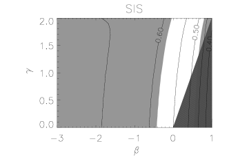
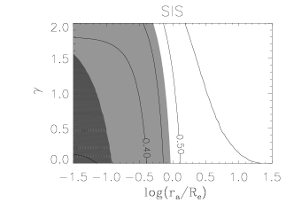
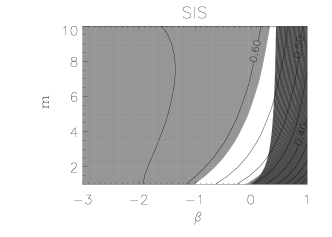
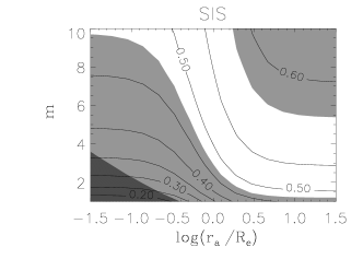
Figure 3: Contours of constant $\log c_{\rm e2}$ in the planes $\beta$-$\gamma$, $\beta$-$m$ (left, for $\beta=const$ models), and $\log(r_{\rm a}/R_{\rm e})$-$\gamma$, $\log(r_{\rm a}/R_{\rm e})$-$m$ (right, for OM models), for systems with singular isothermal sphere total mass distribution. Dark-shaded regions correspond to non-consistent models. Light-shaded regions are outside the observed range $\langle\log c_{\rm e2}\rangle=0.53\pm 0.057$ (Bolton et al., 2008b).

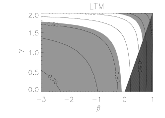
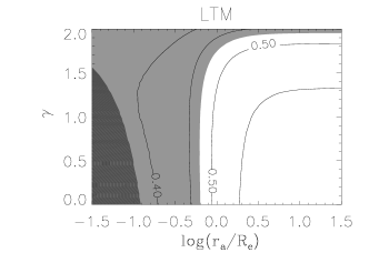
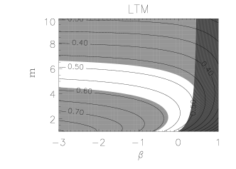
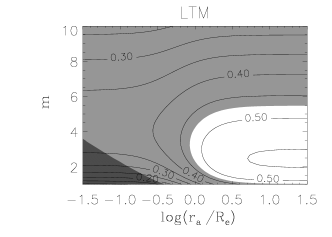
Figure 4: Same as Fig. 3, but for light-traces-mass models.

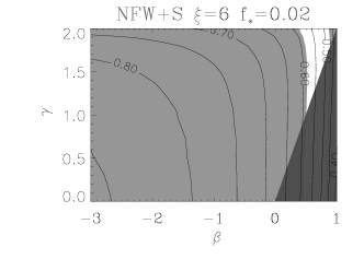
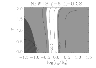
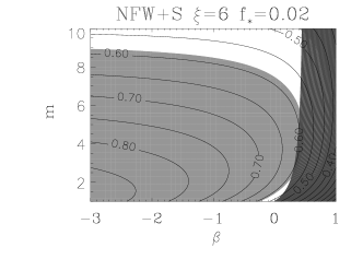
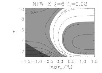
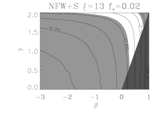
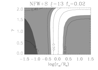
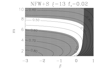
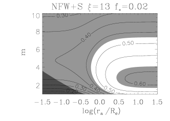
Figure 5: Same as Fig. 3, but for NFW plus stars models with $f_{*}=0.02$.

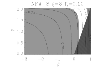
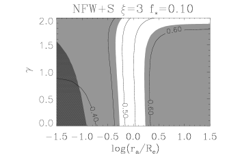
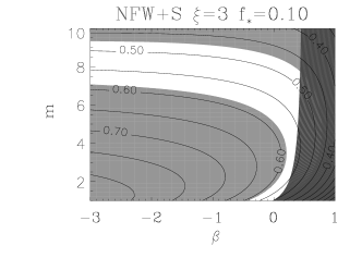
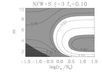
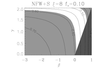
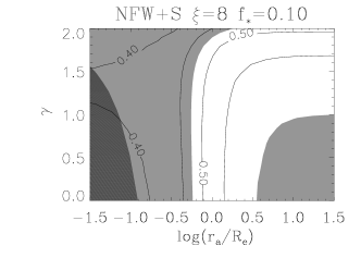
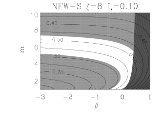
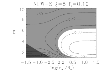
Figure 6: Same as Fig. 3, but for NFW plus stars models with $f_{*}=0.1$.

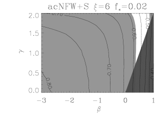
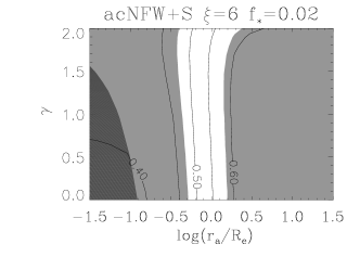
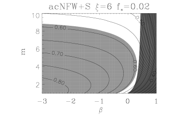
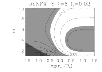
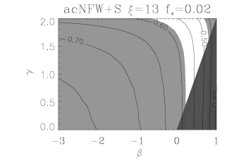
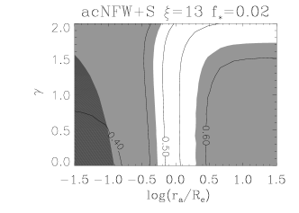
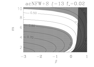
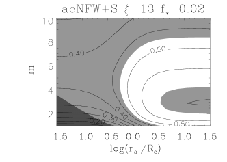
Figure 7: Same as Fig. 3, but for adiabatically contracted NFW plus stars models with $f_{*}=0.02$.

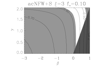
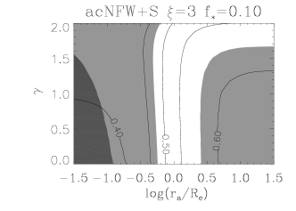
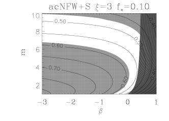
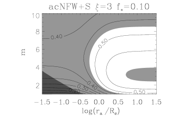
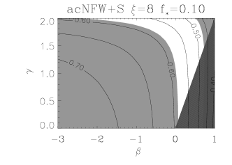
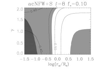
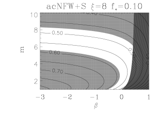
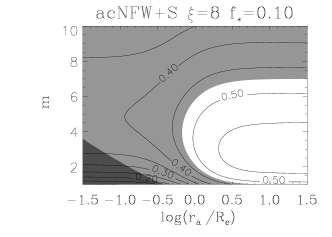
Figure 8: Same as Fig. 3, but for adiabatically contracted NFW plus stars models with $f_{*}=0.1$.

We numerically compute $c_{\rm e2}$ for $\gamma$ models with $0\leq\gamma\leq 2$ and Sérsic models with $1\leq m\leq 10$ for different total mass distributions and orbital anisotropy. Here we discuss how the obtained values of $c_{\rm e2}$ compare with the observed range $\langle\log c_{\rm e2}\rangle=0.53\pm 0.057$ (Bolton et al., 2008b). For each combination of family of stellar systems and total density distribution, we represent our results using contour plots of $\log c_{\rm e2}$ in planes of anisotropy versus stellar profile parameters (Figs. 3-8): $\beta$-$\gamma$ for $\beta=\mathit{const}$ $\gamma$ models, $\beta$-$m$ for $\beta=\mathit{const}$ Sérsic models, $\log(r_{\rm a}/R_{\rm e})$-$\gamma$ for OM $\gamma$ models, and $\log(r_{\rm a}/R_{\rm e})$-$m$ for OM Sérsic models. In such plots, “allowed” regions are white, regions corresponding to non-consistent models are dark-shaded, while regions outside the observed range are light-shaded.

OM models that are unphysical because non-consistent (dark-shaded areas in the right-hand columns of Figs. 3-8) are also outside the observed range. On the other hand, there are non-consistent $\beta=\mathit{const}$ models with $c_{\rm e2}$ in the observed range. This different behaviour of OM and $\beta=\mathit{const}$ models is not surprising, because the latter are known to be less realistic than OM models (see Section 2.4), and, in particular, some radially anisotropic $\beta=\mathit{const}$ models turn out to be unphysical because they are radially anisotropic down to the very centre of the system. This finding stresses the importance of investigating consistency when modeling observational data.

At a first level of interpretation, the plots in Figs. 3-8 show that a relatively wide class of models have values of the structure parameter $c_{\rm e2}$ in the observed range. Thus, the fact that the observed values of $c_{\rm e2}$ lie in a small range does not necessarily imply that early-type galaxies are structurally and dynamically homologous. The reason for this is that $c_{\rm e2}$ is not dramatically sensitive to the mass distribution and orbital anisotropy. However, a more detailed analysis of the diagrams indicates that there is also a wide class of models that lie outside the region allowed by the observations. Here we summarize the behaviour of families of models with different total mass distribution:

• SIS models (Fig. 3): SIS models are consistent with observational constraints for a wide class of stellar density profile and anisotropy. All isotropic $\gamma$ models and isotropic Sérsic models with $m{\,\mathrel{\mathchoice{\lower 2.9pt\vbox{\halign{$\m@th\displaystyle\hfil#\hfil$\cr<\crcr\sim\crcr}}}{\lower 2.9pt\vbox{\halign{$\m@th\textstyle\hfil#\hfil$\cr<\crcr\sim\crcr}}}{\lower 2.9pt\vbox{\halign{$\m@th\scriptstyle\hfil#\hfil$\cr<\crcr\sim\crcr}}}{\lower 2.9pt\vbox{\halign{$\m@th\scriptscriptstyle\hfil#\hfil$\cr<\crcr\sim\crcr}}}\,}}5.5$ have $c_{\rm e2}$ within the observed range. Higher-$m$ Sérsic models can be reconciled with the observations if their stars have radially-biased orbits. Strong radial and tangential anisotropy is excluded. However, very strong radial anisotropy should be excluded on the basis of consistency arguments, while, as briefly discussed in Section 2.4, very strong tangential anisotropy is not expected. One might speculate that the OM models excluded by the observed range trace roughly the region of radially unstable models (see Section 2.5).

• LTM models (Fig. 4): isotropic (and mildly radially anisotropic) $\gamma$ models with LTM potential are consistent with the observational constraints, while isotropic (and mildly radially anisotropic) Sérsic models with LTM potential are acceptable only for $m{\,\mathrel{\mathchoice{\lower 2.9pt\vbox{\halign{$\m@th\displaystyle\hfil#\hfil$\cr<\crcr\sim\crcr}}}{\lower 2.9pt\vbox{\halign{$\m@th\textstyle\hfil#\hfil$\cr<\crcr\sim\crcr}}}{\lower 2.9pt\vbox{\halign{$\m@th\scriptstyle\hfil#\hfil$\cr<\crcr\sim\crcr}}}{\lower 2.9pt\vbox{\halign{$\m@th\scriptscriptstyle\hfil#\hfil$\cr<\crcr\sim\crcr}}}\,}}5.5$. In contrast with the case of SIS models, there is no way of reconciling $m{\,\mathrel{\mathchoice{\lower 2.9pt\vbox{\halign{$\m@th\displaystyle\hfil#\hfil$\cr>\crcr\sim\crcr}}}{\lower 2.9pt\vbox{\halign{$\m@th\textstyle\hfil#\hfil$\cr>\crcr\sim\crcr}}}{\lower 2.9pt\vbox{\halign{$\m@th\scriptstyle\hfil#\hfil$\cr>\crcr\sim\crcr}}}{\lower 2.9pt\vbox{\halign{$\m@th\scriptscriptstyle\hfil#\hfil$\cr>\crcr\sim\crcr}}}\,}}6.5$ Sérsic models with the observations. As in the case of SIS models, the lower limit on $r_{\rm a}/R_{\rm e}$ for OM models might be determined by radial-orbit instability. More tangential anisotropy than in SIS models is allowed, though with some fine-tuning with the stellar profile parameters $m$ and $\gamma$. Curiously, if one considers $\gamma=2$ models under the assumption of LTM and constant anisotropy, the observational constraints would favour tangential with respect to radial anisotropy.

• NFW+S models (Figs. 5 and 6): for some NFW+S models only remarkably small regions of the parameter space are allowed, in contrast with the case of SIS models. The worst case is that of more dark-matter dominated models ($f_{*}=0.02$, $\xi=6$): remarkably, isotropic $\gamma$ models are excluded, and isotropic Sérsic models are allowed only for $m{\,\mathrel{\mathchoice{\lower 2.9pt\vbox{\halign{$\m@th\displaystyle\hfil#\hfil$\cr>\crcr\sim\crcr}}}{\lower 2.9pt\vbox{\halign{$\m@th\textstyle\hfil#\hfil$\cr>\crcr\sim\crcr}}}{\lower 2.9pt\vbox{\halign{$\m@th\scriptstyle\hfil#\hfil$\cr>\crcr\sim\crcr}}}{\lower 2.9pt\vbox{\halign{$\m@th\scriptscriptstyle\hfil#\hfil$\cr>\crcr\sim\crcr}}}\,}}7.5$). Better is the most baryon dominated case ($f_{*}=0.1$, $\xi=8$), which—as expected—behaves similarly to the LTM case, so OM Sérsic models can be reconciled with the observations only for $m{\,\mathrel{\mathchoice{\lower 2.9pt\vbox{\halign{$\m@th\displaystyle\hfil#\hfil$\cr<\crcr\sim\crcr}}}{\lower 2.9pt\vbox{\halign{$\m@th\textstyle\hfil#\hfil$\cr<\crcr\sim\crcr}}}{\lower 2.9pt\vbox{\halign{$\m@th\scriptstyle\hfil#\hfil$\cr<\crcr\sim\crcr}}}{\lower 2.9pt\vbox{\halign{$\m@th\scriptscriptstyle\hfil#\hfil$\cr<\crcr\sim\crcr}}}\,}}6$. In some cases (e.g. OM Sérsic NFW+S models) the anisotropy and stellar-profile parameters must be fine-tuned in order to have $c_{\rm e2}$ in the observed range. For NFW+S models with acceptable $c_{\rm e2}$ we find $0.1{\,\mathrel{\mathchoice{\lower 2.9pt\vbox{\halign{$\m@th\displaystyle\hfil#\hfil$\cr<\crcr\sim\crcr}}}{\lower 2.9pt\vbox{\halign{$\m@th\textstyle\hfil#\hfil$\cr<\crcr\sim\crcr}}}{\lower 2.9pt\vbox{\halign{$\m@th\scriptstyle\hfil#\hfil$\cr<\crcr\sim\crcr}}}{\lower 2.9pt\vbox{\halign{$\m@th\scriptscriptstyle\hfil#\hfil$\cr<\crcr\sim\crcr}}}\,}}f_{\rm dm}{\,\mathrel{\mathchoice{\lower 2.9pt\vbox{\halign{$\m@th\displaystyle\hfil#\hfil$\cr<\crcr\sim\crcr}}}{\lower 2.9pt\vbox{\halign{$\m@th\textstyle\hfil#\hfil$\cr<\crcr\sim\crcr}}}{\lower 2.9pt\vbox{\halign{$\m@th\scriptstyle\hfil#\hfil$\cr<\crcr\sim\crcr}}}{\lower 2.9pt\vbox{\halign{$\m@th\scriptscriptstyle\hfil#\hfil$\cr<\crcr\sim\crcr}}}\,}}0.6$ and $0.2{\,\mathrel{\mathchoice{\lower 2.9pt\vbox{\halign{$\m@th\displaystyle\hfil#\hfil$\cr<\crcr\sim\crcr}}}{\lower 2.9pt\vbox{\halign{$\m@th\textstyle\hfil#\hfil$\cr<\crcr\sim\crcr}}}{\lower 2.9pt\vbox{\halign{$\m@th\scriptstyle\hfil#\hfil$\cr<\crcr\sim\crcr}}}{\lower 2.9pt\vbox{\halign{$\m@th\scriptscriptstyle\hfil#\hfil$\cr<\crcr\sim\crcr}}}\,}}f_{\rm dm}^{\rm p}{\,\mathrel{\mathchoice{\lower 2.9pt\vbox{\halign{$\m@th\displaystyle\hfil#\hfil$\cr<\crcr\sim\crcr}}}{\lower 2.9pt\vbox{\halign{$\m@th\textstyle\hfil#\hfil$\cr<\crcr\sim\crcr}}}{\lower 2.9pt\vbox{\halign{$\m@th\scriptstyle\hfil#\hfil$\cr<\crcr\sim\crcr}}}{\lower 2.9pt\vbox{\halign{$\m@th\scriptscriptstyle\hfil#\hfil$\cr<\crcr\sim\crcr}}}\,}}0.7$, where $f_{\rm dm}$ and $f_{\rm dm}^{\rm p}$ are, respectively, the intrinsic and projected dark-matter-to-total mass ratios within $R_{\rm e}$.

• acNFW+S models (Figs. 7 and 8): overall, adiabatically contracted models behave similarly to non-contracted models, but allowed regions in the parameter space are slightly more extended in acNFW+S models than in the corresponding NFW+S models. As in the case of NFW+S, baryon-dominated models (larger values of $f_{*}$ and $\xi$) are more successful than dark-matter dominated models (smaller values of $f_{*}$ and $\xi$). However, acNFW+S have some of the same undesirable features present in NFW+S models, such as a wide class of unacceptable isotropic models (especially when $f_{*}=0.02$). For dark-matter dominated OM Sérsic acNFW+S models to have $c_{\rm e2}$ in the observed range, the anisotropy and stellar-profile parameters must be fine-tuned. The acNFW+S models with $c_{\rm e2}$ within the observed range have $0.3{\,\mathrel{\mathchoice{\lower 2.9pt\vbox{\halign{$\m@th\displaystyle\hfil#\hfil$\cr<\crcr\sim\crcr}}}{\lower 2.9pt\vbox{\halign{$\m@th\textstyle\hfil#\hfil$\cr<\crcr\sim\crcr}}}{\lower 2.9pt\vbox{\halign{$\m@th\scriptstyle\hfil#\hfil$\cr<\crcr\sim\crcr}}}{\lower 2.9pt\vbox{\halign{$\m@th\scriptscriptstyle\hfil#\hfil$\cr<\crcr\sim\crcr}}}\,}}f_{\rm dm}{\,\mathrel{\mathchoice{\lower 2.9pt\vbox{\halign{$\m@th\displaystyle\hfil#\hfil$\cr<\crcr\sim\crcr}}}{\lower 2.9pt\vbox{\halign{$\m@th\textstyle\hfil#\hfil$\cr<\crcr\sim\crcr}}}{\lower 2.9pt\vbox{\halign{$\m@th\scriptstyle\hfil#\hfil$\cr<\crcr\sim\crcr}}}{\lower 2.9pt\vbox{\halign{$\m@th\scriptscriptstyle\hfil#\hfil$\cr<\crcr\sim\crcr}}}\,}}0.65$ and $0.35{\,\mathrel{\mathchoice{\lower 2.9pt\vbox{\halign{$\m@th\displaystyle\hfil#\hfil$\cr<\crcr\sim\crcr}}}{\lower 2.9pt\vbox{\halign{$\m@th\textstyle\hfil#\hfil$\cr<\crcr\sim\crcr}}}{\lower 2.9pt\vbox{\halign{$\m@th\scriptstyle\hfil#\hfil$\cr<\crcr\sim\crcr}}}{\lower 2.9pt\vbox{\halign{$\m@th\scriptscriptstyle\hfil#\hfil$\cr<\crcr\sim\crcr}}}\,}}f_{\rm dm}^{\rm p}{\,\mathrel{\mathchoice{\lower 2.9pt\vbox{\halign{$\m@th\displaystyle\hfil#\hfil$\cr<\crcr\sim\crcr}}}{\lower 2.9pt\vbox{\halign{$\m@th\textstyle\hfil#\hfil$\cr<\crcr\sim\crcr}}}{\lower 2.9pt\vbox{\halign{$\m@th\scriptstyle\hfil#\hfil$\cr<\crcr\sim\crcr}}}{\lower 2.9pt\vbox{\halign{$\m@th\scriptscriptstyle\hfil#\hfil$\cr<\crcr\sim\crcr}}}\,}}0.75$.

Summarizing, our results indicate that the tightness of the MP requires some degree of “fine tuning” in the internal properties of early-type galaxies. Although no family of models is strictly ruled out, some families of models allow for more freedom in the remaining parameters describing, e.g., the luminous profile and stellar orbits. The tightness of the MP is well consistent with the hypothesis that the total mass profile is that of a SIS, allowing a broad range of values for the other parameters. The LTM hypothesis is acceptable if early-type galaxies have intrinsic stellar density profiles described by $\gamma$ models or Sérsic projected stellar density profiles with index $m{\,\mathrel{\mathchoice{\lower 2.9pt\vbox{\halign{$\m@th\displaystyle\hfil#\hfil$\cr<\crcr\sim\crcr}}}{\lower 2.9pt\vbox{\halign{$\m@th\textstyle\hfil#\hfil$\cr<\crcr\sim\crcr}}}{\lower 2.9pt\vbox{\halign{$\m@th\scriptstyle\hfil#\hfil$\cr<\crcr\sim\crcr}}}{\lower 2.9pt\vbox{\halign{$\m@th\scriptscriptstyle\hfil#\hfil$\cr<\crcr\sim\crcr}}}\,}}5.5$. For either non-contracted or adiabatically contracted NFW cases, baryon-dominated models require less fine-tuning than dark-matter-dominated models. In general, isotropic or mildly radially anisotropic velocity distribution is easier to reconcile with the MP than tangential or extremely radial anisotropy.

4 Sérsic index and the tilt of the Mass Plane

In the previous Section we have interpreted the average value and intrinsic scatter of the parameter $c_{\rm e2}$ describing the MP. In this Section we consider how future observations of the MP over a broader range of galaxy masses could be used to further constrain the internal structure of early-type galaxies, based on the known structural non-homology of their luminous component.

The Sérsic index $m$ of early-type galaxies correlates with galaxy size, in the sense that more extended galaxies have higher $m$ (Caon, Capaccioli & D’Onofrio, 1993; Graham & Guzmán, 2003; Ferrarese et al., 2006): in particular, Caon, Capaccioli & D’Onofrio (1993) found

$$\log m=0.28+0.52\log\left({R_{\rm e}\over{\rm\,kpc}}\right).$$ (31)

As the effective radius increases with galaxy luminosity (e.g. Bernardi et al., 2003a), equation (31) should imply a correlation between $m$ and luminosity. For example, using surface photometry from the well-defined Virgo Cluster sample of Ferrarese et al. (2006), we obtain the following relation

$$\log m=(0.27\pm 0.02)\log\left({{\rm L}_{\rm B}\over{\rm L}_{{\rm B},\odot}}\right)-(2.07\pm 0.02)$$ (32)

where ${\rm L}_{\rm B}$ is the B-band luminosity obtained from the ACS filters as described by Gallo et al. (2008), and the uncertainties on the best-fit coefficients are 1 $\sigma$ (the RMS scatter about the relation is 0.16 dex). Such a systematic variation of $m$ with luminosity could at least partly contribute to the observed tilt of the FP of early-type galaxies (Hjorth & Madsen, 1995; Ciotti & Lanzoni, 1997; Graham & Colless, 1997; Bertin, Ciotti & Del Principe, 2002; Trujillo, Burkert & Bell, 2004; Cappellari et al., 2006). If the stellar mass contributes significantly to the projected mass within $R_{\rm e}/2$—as is generally assumed and as supported by the modeling results above—the dependence of $m$ on luminosity could introduce a tilt in the MP. This would in turn induce a tilt in the relation between $M_{\rm e2}^{\rm p}\equiv M_{\rm tot}^{\rm p}(R_{\rm e}/2)$ and $M^{\rm dim}_{\rm e2}\equiv R_{\rm e}\sigma_{\rm e2}^{2}/(2G)$, because the structure parameter $c_{\rm e2}$ depends on $m$ for given total mass distribution and orbital anisotropy. For the massive galaxies studied in their sample, Bolton et al. (2008b) found

$$\log\left({M_{\rm e2}^{\rm p}\over 10^{11}M_{\odot}}\right)=\delta\left({M^{\rm dim}_{\rm e2}\over 10^{11}M_{\odot}}\right)+\log c_{\rm e2},$$ (33)

with $\log c_{\rm e2}=0.54\pm 0.02$ and $\delta=1.03\pm 0.04$. Note that here we are not considering the average value of $\log c_{\rm e2}$ as in equation (4), but rather are accounting for a possible dependence of $c_{\rm e2}$ on mass. A deviation of $\delta$ from unity is a signature of tilt, so the observational data are consistent with absence of tilt. Actually Bolton et al. (2008b) found no correlation between galaxy mass/luminosity and Sérsic index in their sample, consistent with the fact that the SLACS sample is confined to a relatively small range of galaxy luminosities towards the bright end of the luminosity function of early-type galaxies: the mass range of Bolton et al.’s sample is $10.3{\,\mathrel{\mathchoice{\lower 2.9pt\vbox{\halign{$\m@th\displaystyle\hfil#\hfil$\cr<\crcr\sim\crcr}}}{\lower 2.9pt\vbox{\halign{$\m@th\textstyle\hfil#\hfil$\cr<\crcr\sim\crcr}}}{\lower 2.9pt\vbox{\halign{$\m@th\scriptstyle\hfil#\hfil$\cr<\crcr\sim\crcr}}}{\lower 2.9pt\vbox{\halign{$\m@th\scriptscriptstyle\hfil#\hfil$\cr<\crcr\sim\crcr}}}\,}}\log(M_{\rm e2}^{\rm p}/M_{\odot}){\,\mathrel{\mathchoice{\lower 2.9pt\vbox{\halign{$\m@th\displaystyle\hfil#\hfil$\cr<\crcr\sim\crcr}}}{\lower 2.9pt\vbox{\halign{$\m@th\textstyle\hfil#\hfil$\cr<\crcr\sim\crcr}}}{\lower 2.9pt\vbox{\halign{$\m@th\scriptstyle\hfil#\hfil$\cr<\crcr\sim\crcr}}}{\lower 2.9pt\vbox{\halign{$\m@th\scriptscriptstyle\hfil#\hfil$\cr<\crcr\sim\crcr}}}\,}}12$. We thus compute the tilt to determine whether it is measurable and could lead to further discriminatory power if one considered a sample covering a larger mass range. For this purpose, we use our models to quantify the tilt introduced in the MP by the expected dependence of $m$ on mass. We consider our models with Sérsic stellar distributions and we map $m$ into $M_{\rm e2}^{\rm p}$ by combining equation (32) with the best-fit correlation (Bolton et al., 2008b)

$$\log\left({L_{\rm V}\over 10^{11}L_{{\rm V}\odot}}\right)=0.73\log\left({M_{\rm e2}^{\rm p}\over 10^{11}M_{\odot}}\right)-0.24,$$ (34)

assuming $B-V=0.96$ (Fukugita et al., 1995). In order to isolate the effect of the structural non-homology of the stellar distribution, it is useful to compare models under the same assumptions on the velocity distribution. In this Section we focus on models with radial anisotropy with OM parameterization. We consider two families of OM models with values of $r_{\rm a}/R_{\rm e}$ independent of $m$: isotropic models ($r_{\rm a}/R_{\rm e}=\infty$) and radially anisotropic models with $r_{\rm a}=R_{\rm e}$. As for the FP, dynamical non-homology might contribute to produce a tilt of the MP, so it is important to consider also the case in which more massive (higher-$m$) system are more radially anisotropic than less massive (lower-$m$) systems. This choice is motivated by the fact that higher-$m$ system can sustain more radial anisotropy than lower-$m$ systems (see Section 2.5 and Figs. 3-8) and by previous studies on the FP (e.g. Ciotti, Lanzoni & Renzini, 1996; Ciotti & Lanzoni, 1997; Nipoti, Londrillo & Ciotti, 2002). Thus, we also consider a family of models in which $\log r_{\rm a}/R_{\rm e}=0.1(10-m)-0.3$: with this parameterization $m\sim 1$ systems are almost isotropic, while $m\sim 10$ systems are strongly radially anisotropic. In Fig. 9 we plot $M_{\rm e2}^{\rm p}/M^{\rm dim}_{\rm e2}$ as a function of $M_{\rm e2}^{\rm p}$ (and of $m$) for OM $R^{1/m}$ models with different total mass distribution and for the three different choices of the value of $r_{\rm a}/R_{\rm e}$ (isotropic in the left-hand panels, $r_{\rm a}=R_{\rm e}$ in the central panels and $r_{\rm a}/R_{\rm e}$ depending on $m$ in the right-hand panels). In each panel the dashed line and the dotted lines are, respectively, the best-fit observed relation (equation 33 with $\log c_{\rm e2}=0.54$ and $\delta=1.03$), and the associated scatter in $\delta$ and $\log c_{\rm e2}$. In Fig. 9 we report plots for the SIS, LTM and acNFW+S models. We note that the acNFW+S models considered in this case have fixed value of $f_{*}$ ($f_{*}=0.1$ or $f_{*}=0.02$), but the value of $\xi$ is a function of $m$: for given $m$ we obtain $R_{\rm e}$ from the observed relation (31) and then $\xi$ from equation (24), fixing $C_{200}=8$.

From the diagrams in Fig. 9 it is apparent that the SIS models behave very differently from the LTM and acNFW+S models (NFW+S models, which are not plotted, behave similarly to acNFW models). Let us focus first on the case with $r_{\rm a}/R_{\rm e}$ independent of $m$ (left-hand and central panels in Fig. 9). For the SIS model the ratio $M_{\rm e2}^{\rm p}/M^{\rm dim}_{\rm e2}$ gradually increases with $M_{\rm e2}^{\rm p}$, while for all other models the ratio $M_{\rm e2}^{\rm p}/M^{\rm dim}_{\rm e2}$ increases with $M_{\rm e2}^{\rm p}$ at low masses and decreases with $M_{\rm e2}^{\rm p}$ at high masses (in sharp contrast with the tilt predicted for SIS models), and the variations with $M_{\rm e2}^{\rm p}$ are stronger than in the case of the SIS models. Quantitatively, at high masses, the predicted slope $\delta$ of equation (33) is $\delta>1$ for SIS models and $\delta<1$ for the other models. When $r_{\rm a}/R_{\rm e}$ depends on $m$ (right-hand panels in Fig. 9), the dynamical non-homology introduces additional tilt, in the sense that the predicted value of $\delta$ at high masses becomes smaller, giving $\delta<1$ also for SIS models. However, also in this case significantly less tilt is predicted for the SIS models with respect to the other models.

In conclusion, the effect of structural non-homology on the tilt of the MP is of order of a tenth of a dex in the mass ratio and thus measurable if one had a sample comparable in size and quality to SLACS, covering a further decade down in galaxy masses. Interestingly, the tilt of the MP is measurably different depending on whether or not the total mass profile is well represented by a SIS. The tilt of the MP appears thus to be a powerful diagnostic of the internal structure of early-type galaxies.

5 Summary and conclusions

In the range $\sigma_{\rm e2}=175-400$ km s^-1 the MP of early-type galaxies has no significant tilt and small associated scatter. This means that the dimensionless structure parameter $c_{\rm e2}$ defined in equation (3) is a nearly universal constant. In other words, the range of values of $c_{\rm e2}$ “allowed” by the observational data is remarkably small. Even for spherical galaxy models, $c_{\rm e2}$ is expected to depend on the stellar density profile, orbital anisotropy of stars, and total (dark plus luminous) mass distribution. In this paper we explored the constraints posed by the existence of the MP on several relevant families of galaxy models.

Limiting to spherically symmetric models, we found that $c_{\rm e2}$ is not very strongly dependent on galaxy structure and kinematics, so a relatively wide class of models have values of $c_{\rm e2}$ within the observed range. Therefore, strictly speaking, the massive early-type galaxies lying on the MP are not necessarily structurally and dynamical homologous. However, not all the studied models behave in the same way when compared to the observational data. Models in which the total density profile is a SIS are consistent with the observed range of $c_{\rm e2}$ for a wide class of stellar density profiles, and only models with extremely radial or tangential anisotropies are excluded. The light-traces-mass hypothesis is not excluded by the observational constraints here considered, apart for the case of high-$m$ Sérsic models, which cannot be reconciled with the MP within the observed scatter. (However, LTM models are known to fail other observational constraints: see Section 2.3). We also considered cosmologically-motivated models with NFW dark-matter halos (with or without adiabatic compression), finding that they are consistent with the MP only for a relatively limited range of values of their parameters, so a degree of fine-tuning between light profile and anisotropy is required. Among these NFW models, those with adiabatically contracted halos and those that are baryon dominated seem to require slightly less fine tuning than those with non-contracted halos and those that are dark-matter dominated.

This work has focused on the average value of $c_{\rm e2}$ in the SLACS sample, along with its intrinsic scatter. With the exception of Section 4, we have not explored the implications of the fact that this intrinsic scatter is not correlated with either mass or with the ratio of Einstein radius to $R_{\rm e}$ (Bolton et al., 2008b). These observational results indicate a degree of structural homogeneity across a range in mass. In future works, we will explore these mass-dependent results in the context of mass-dynamical models such as those considered here. We also plan to refine these analyses based on the results of forthcoming velocity-dispersion measurements of higher signal-to-noise ratio and in smaller and more uniform spatial apertures.

We also explored the possibility that the observed dependence of the Sérsic index $m$ on the galaxy luminosity could tilt the MP when a sufficiently large mass range is considered. In this respect, SIS models behave differently from all other models: a slightly tilted MP is predicted in the early type galaxies have SIS total density distribution, while a “bent” MP is predicted in all the other explored cases. The effect is large enough to be measurable with sample of lenses comparable to SLACS in size and quality and extending a further decade in galaxy mass.

In conclusion, our results are consistent with the hypothesis that massive early-type galaxies have isothermal ($\propto r^{-2}$) total mass density distribution, though alternative hypotheses cannot be excluded on the basis of the existence of the MP alone, although in some cases they require a degree of fine tuning. In any case, the process of formation of early-type galaxies lead to systems with a combination of total mass distribution, luminosity profile, and orbital anisotropy such that they lie close to the MP. It will be interesting to quantify whether the observed fine tuning is quantitatively consistent with the range of simulated properties of early-type galaxies in the standard hierarchical model of galaxy formation.

Figure 9: Ratio between the total projected mass within $R_{\rm e}/2$ ($M_{\rm e2}^{\rm p}$) and the dimensional mass $M^{\rm dim}_{\rm e2}=R_{\rm e}\sigma_{\rm e2}^{2}/(2G)$ as a function of $M_{\rm e2}^{\rm p}$ for $R^{1/m}$ Sérsic spherical OM galaxy models with different total mass distributions and values of $r_{\rm a}/R_{\rm e}$. In each panel the dashed line is the best-fit observed relation with the associated scatter (dotted lines) found by Bolton et al. (2008b, see text for details).

References

- An & Evans (2006) An J.H., Evans N.W., 2006, ApJ, 642, 752
- Barnes (1992) Barnes J.E., 1992, ApJ, 393, 484
- Bender, Burstein & Faber (1992) Bender R., Burstein D., Faber S.M., 1992, ApJ, 399, 462
- Bernardi et al. (2003a) Bernardi M., et al. 2003a, AJ, 125, 1849
- Bernardi et al. (2003b) Bernardi M. et al., 2003b, AJ, 125, 1866
- Bertin & Stiavelli (1989) Bertin G., Stiavelli M., 1989, ApJ, 338, 723
- Bertin et al. (1994) Bertin G. et al., 1994, A&A, 292, 381
- Bertin, Ciotti & Del Principe (2002) Bertin G., Ciotti L., Del Principe M., 2002, A&A, 386, 1491
- Binney & Mamon (1982) Binney J., Mamon G.A., 1982, MNRAS, 200, 361
- Binney & Tremaine (2008) Binney J., Tremaine S., 2008, Galactic Dynamics 2nd Ed., Princeton University Press, Princeton
- Blumenthal et al. (1986) Blumenthal G.R., Faber S.M., Flores R., Primack J.R., 1986, ApJ, 301, 27
- Bolton et al. (2006) Bolton A.S., Burles S., Koopmans L.V.E., Treu T., Moustakas L.A., 2006, ApJ, 638, 703
- Bolton et al. (2007) Bolton A.S., Burles S., Treu T., Koopmans L.V.E., Moustakas L.A., 2007, ApJ, 665, L105
- Bolton et al. (2008a) Bolton A.S., et al. 2008a, ApJ, in press (arXiv:0805.1931)
- Bolton et al. (2008b) Bolton A.S., et al. 2008b, ApJ, in press (arXiv:0805.1932)
- Borriello, Salucci & Danese (2003) Borriello A., Salucci P., Danese L., 2003, MNRAS, 341, 1109
- Caon, Capaccioli & D’Onofrio (1993) Caon N., Capaccioli M., D’Onofrio M., 1993, 265, 1013
- Cappellari et al. (2006) Cappellari M. et al., 2006, MNRAS, 366, 1126
- Cappellari et al. (2007) Cappellari M. et al., 2007, MNRAS, 379, 418
- Ciotti (1991) Ciotti L., 1991, A&A, 249, 99
- Ciotti (1994) Ciotti L., 1994, Celestial Mechanics & Dynamical Astronomy, 60, 401
- Ciotti & Bertin (1999) Ciotti L., Bertin G., 1999, A&A, 352, 447
- Ciotti & Lanzoni (1997) Ciotti L., Lanzoni B., 1997, A&A, 321, 724
- Ciotti & Pellegrini (1992) Ciotti L., Pellegrini S., 1992, MNRAS, 255, 561
- Ciotti, Lanzoni & Renzini (1996) Ciotti L., Lanzoni B., Renzini A., 1996, MNRAS, 282, 1
- Dehnen (1993) Dehnen W., 1993, MNRAS, 265, 250
- de Vaucouleurs (1948) de Vaucouleurs G., 1948, Ann. d’Astroph., 11,247
- Djorgovsky & Davis (1987) Djorgovsky S., Davis M., 1987, ApJ, 313, 59
- Dressler et al. (1987) Dressler A., Faber S.M., Burstein D., Davies R.L., Lynden-Bell D., Terlevich R.J., Wegner, G., 1987, ApJ, 313, 37
- Dye et al. (2007) Dye S., Smail I., Swinbank A.M., Ebeling H., Edge A. C., 2007, MNRAS, 379, 308
- Dye & Warren (2005) Dye S., Warren S. J. 2005, ApJ, 623, 31
- El-Zant et al. (2004) El-Zant A., Hoffman Y., Primack J., Combes F., Shlosman I., 2004, ApJ, 607, L75
- Faber et al. (1987) Faber S.M., Dressler A., Davies R.L., Burstein D., Lynden-Bell D., 1987, in “Nearly normal galaxies: From the Planck time to the present”, New York, Springer-Verlag, 1987, p. 175-183.
- Ferrarese et al. (2006) Ferrarese L., et al., 2006, ApJS, 164, 334
- Fridman & Polyachenko (1984) Fridman A. M., Polyachenko V.L., 1984, Physics of Gravitating Systems (Springer, New York)
- Fukugita et al. (1995) Fukugita M., Shimasaku K., Ichikawa T., 1995, PASP, 107, 945
- Gallo et al. (2008) Gallo E., Treu T., Jacob J., Woo J.-H., Marshall P.J., Antonucci R., 2008, ApJ, 680, 154
- Gavazzi et al. (2007) Gavazzi R. et al., 2007, ApJ, 667, 176
- Gavazzi et al. (2008) Gavazzi R. et al., 2008, ApJ, 677, 1046
- Gerhard et al. (2001) Gerhard O., Kronawitter A., Saglia R.P., Bender R., 2001, AJ, 121, 1936
- Gnedin et al. (2004) Gnedin O.Y., Kravtsov A.V., Klypin A.A., Nagai D., 2004, ApJ, 616, 16
- Graham & Colless (1997) Graham A.W., Colless M., 1997, MNRAS, 287, 221
- Graham & Guzmán (2003) Graham A.W., Guzmán R., 2003, AJ, 125, 2936
- Hernquist (1990) Hernquist L., 1990, ApJ, 356, 359
- Hernquist (1993) Hernquist L., 1993, ApJ, 409, 548
- Hjorth & Madsen (1995) Hjorth J., Madsen J., 1995, ApJ, 445, 55
- Jaffe (1983) Jaffe W., 1983, MNRAS, 202, 995
- Jiang & Kochanek (2007) Jiang G., Kochanek C.S., 2007, ApJ, 671, 1568
- Keeton (2001) Keeton C.R, 2001, 561, 46
- Kochanek (1994) Kochanek C.S., 1994, ApJ, 436, 56
- Koopmans & Treu (2002) Koopmans L.V.E., Treu T., 2002, ApJ, 568, L5
- Koopmans & Treu (2003) Koopmans L.V.E., Treu T., 2003, ApJ, 583, 606
- Koopmans et al. (2006) Koopmans L.V., Treu T., Bolton A.S., Burles S., Moustakas L.A., 2006, ApJ, 649, 599
- Kronawitter et al. (2000) Kronawitter A., Saglia R.P., Gerhard O., Bender R., 2000, A&AS, 144, 53
- Lanzoni & Ciotti (2003) Lanzoni B., Ciotti L., 2003, A&A, 404, 819
- Merritt (1985) Merritt D., 1985, AJ, 90, 102
- Merritt & Aguilar (1985) Merritt D., Aguilar L.A., 1985, MNRAS, 217, 787
- Meza & Zamorano (1997) Meza A., Zamorano N., 1997, AJ, 490, 136
- Navarro, Frenk & White (1996) Navarro J.F., Frenk C.S., White S.D.M. 1996, ApJ, 462, 563 (NFW)
- Neto et al. (2007) Neto A.F. et al., 2007, MNRAS, 381, 1450
- Nipoti, Londrillo & Ciotti (2002) Nipoti C., Londrillo P., Ciotti L., 2002, MNRAS, 332, 901
- Nipoti et al. (2004) Nipoti C., Treu T., Ciotti L., Stiavelli M., 2004, MNRAS, 355, 1119
- Nipoti, Londrillo & Ciotti (2006) Nipoti C., Londrillo P., Ciotti L., 2006, MNRAS, 370, 681
- Osipkov (1979) Osipkov L.P., 1979, Soviet Astron. Lett., 5, 42
- Pahre, Djorgovski & de Carvalho (1998) Pahre M.A., Djorgovski S.G., de Carvalho R.R., 1998, AJ, 116, 1591
- Prugniel & Simien (1994) Prugniel Ph., Simien F., 1994, A&A, 282, L1
- Renzini & Ciotti (1993) Renzini A., Ciotti L., 1993 ApJ, 416, L49
- Richstone & Tremaine (1984) Richstone D.O., Tremaine S., 1984, ApJ, 286, 27
- Riciputi et al. (2005) Riciputi A., Lanzoni B., Bonoli S., Ciotti L., 2005, A&A, 443, 133
- Rusin & Kochanek (2005) Rusin D., Kochanek C.S., 2005, ApJ, 623, 666
- Rusin et al. (2003) Rusin D., Kochanek C.S., Keeton C.R., 2003, ApJ, 595, 29
- Saglia, Bender & Dressler (1993) Saglia R.P., Bender R., Dressler A., 1993, A&A, 279, 75
- Saha (1991) Saha P., 1991, MNRAS, 148, 494
- Sanders & Land (2008) Sanders R.H., Land D.D., 2008, submitted to MNRAS (arXiv:0803.0468)
- Sérsic (1968) Sérsic J.L., 1968, Atlas de galaxias australes. Observatorio Astronomico, Cordoba
- Shen et al. (2003) Shen S., Mo H.J., White S.D.M., Blanton M.R., Kauffmann G., Voges W., Brinkmann J., Csabai I., 2003, MNRAS, 343, 978
- Stiavelli & Sparke (1991) Stiavelli M., Sparke L.S., 1991, ApJ, 382, 466
- Tremaine et al. (1994) Tremaine S., Richstone D.O., Yong-Ik B., Dressler A., Faber S.M., Grillmair C., Kormendy J., Laurer T.R., 1994, AJ, 107, 634
- Treu & Koopmans (2002) Treu T., Koopmans L.V.E., 2002, ApJ, 575, 87
- Treu & Koopmans (2003) Treu T., Koopmans L.V.E., 2003, MNRAS, 343, L29
- Treu & Koopmans (2004) Treu T., Koopmans L.V.E., 2004, ApJ, 611, 739
- Treu et al. (2006) Treu T., Koopmans L.V., Bolton A.S., Burles S., Moustakas L.A., 2006, ApJ, 640, 662
- Treu et al. (2008) Treu T., Gavazzi R., Gorecki A., Marshall P.J., Koopmans L.V.E., Bolton A.S., Moustakas L.A., Burles S., 2008, ApJ, submitted (arXiv:0806.1056v1)
- Trujillo, Burkert & Bell (2004) Trujillo I., Burkert A., Bell E.F., 2004, ApJ, 600, L39
- van Albada (1982) van Albada T.S., 1982, MNRAS, 201, 939
- Wayth et al. (2005) Wayth R.B., Warren S.J., Lewis G.F., Hewett P.C., 2005, MNRAS, 360, 1333