Entropies in case of continuous time

Abstract

Information theory on a time-discrete setting in the framework of time series analysis is generalized to the time-continuous case. Considerations of the Roessler and Lorenz dynamics as well as the Ornstein-Uhlenbeck process yield for time-continuous entropies a new possibility for the distinction of chaos and noise. In the deterministic case an upper threshold of the joint uncertainty in the limit of infinitely high sampling rate can be found and the entropy rate can be calculated as a usual time derivative of the entropy. In a three-dimensional representation the dependence of the joint entropy $H(\epsilon,\tau,t)$ on space resolution, discretization time step length and uncertainty-assessed time is shown in a unified manner. Hence the dimension and the Kolmogorov-Sinai entropy rate of any dynamics can be read out as limit cases from one single graph.

I Introduction

Uncertainty of the outcome of random variables $X$ is usually evaluated by Shannon entropies cover91

$$H(X)=-\sum_{i=1}^{N}P(x_{i})\ln P(x_{i})\;,$$ (1)

where $x_{i}$ are the possible realizations of $X$. Relaxing the restrictions in the underlying Khinchin or Fadeev axioms it is possible to introduce the family of Renyi entropies renyi61

$$H^{(q)}(X)=\frac{1}{1-q}\ln\sum_{i=1}^{N}P(x_{i})^{q}\;,$$ (2)

which in the case of Renyi order $q=2$ are quite often used for estimation of entropies via the correlation sum grassproc83 . In the case of time series analysis it is a common task to evaluate the uncertainty of $m$ random variables belonging to $m$ successive time steps kantzschreiber04 . The corresponding joint entropy in the suitable notational representation reads

$$H_{m}^{(q)}(\epsilon,\tau)=\frac{1}{1-q}\ln\left[\sum_{i_{1}=1}^{M_{1}(\epsilon)}...\sum_{i_{m}=1}^{M_{m}(\epsilon)}{(P_{i_{1},...,i_{m}}(\epsilon,\tau))}^{q}\right]\;.$$ (3)

In this expression $\epsilon$ is the space resolution and $\tau$ is the step length of the time discretization. After having decided for a suitable Renyi order, it is often omitted. Now the finite-m-entropy rate can be defined as

$$h_{m}(\epsilon,\tau):=\frac{H_{1|m}(\epsilon,\tau)}{\tau}:=\frac{H_{m+1}(\epsilon,\tau)-H_{m}(\epsilon,\tau)}{\tau}\;.$$ (4)

This quantity is a special conditional entropy per time step length. Since obviously this entropy rate is obtained from a quotient of differences, a time-continuous formulation of the relationships of entropic quantities should naturally also be at hand. The idea of connection of the entropic quantities by derivatives is also supported in crutch03 , where however, the time discretization step length $\tau$ is still kept finite. The questions of consequences of variable time step length $\tau$ and especially the limit of $\tau\rightarrow 0$ for entropic quantities are addressed in this paper and it is intended to give theoretical insights into the structure of the relationships behind such entropic quantities. With those efforts this paper tries to contribute to a symmetrization of the treatment of entropies concerning space, where continuity is already realized in formulas, and time.

First, the line of thought from joint Shannon entropies to the Kolmogorov-Sinai entropy rate is outlined in sec. II, staying quite close to the paper of Gaspard and Wang gaspard93 , the central paper behind this work. The limit of infinitesimal time step length $\tau$ is performed after having performed the limit of infinite time $t=m\tau$. Theoretically, sec. III contains the central aim of this paper. It is the generalization of sec. II with omission of the limit of infinite uncertainty-assessed time $t$, concentrating on the limit of infinitesimal time discretization step length $\tau$. In sec. IV the presented ideas are tested numerically for the examples of the Roessler, Lorenz and Ornstein-Uhlenbeck dynamics with the detection of qualitative discrepancies of deterministic and stochastic dynamics. Sec. V concludes the results of this paper.

II From Shannon entropy to Kolmogorov-Sinai entropy rate

The starting point as given in gaspard93 is the joint Shannon entropy

$$H({\cal{A}},\tau,t)=H_{m:=t/\tau}({\cal{A}},\tau)=-\sum_{\omega_{0},...,\omega_{m-1}}P(\omega_{0},...,\omega_{m-1})\ln P(\omega_{0},...,\omega_{m-1})\;.$$ (5)

The symbol $\tau$, being the time step length, appears on the right side only implicitly as the time between successive realizations and the partition ${\cal{A}}$ appears on the right side implicitly in the range of values $\omega_{k}$, which corresponds to $i$ in eq. (1), can take. In the following it is assumed that the partition for $t_{1}$ is consistent with the partition for $t_{2}>t_{1}$. It is possible to define the rate

$$\tilde{h}({\cal{A}},\tau,t):=\frac{H({\cal{A}},\tau,t)}{t}\;.$$ (6)

The entropy per unit time with respect to partition ${\cal{A}}$ is then defined as the limit

$$\tilde{h}({\cal{A}},\tau):=\lim_{t\rightarrow\infty}\tilde{h}({\cal{A}},\tau,t)\;.$$ (7)

Starting from eq. (5) it is also possible to define another rate

$$h({\cal{A}},\tau,t):=\frac{H({\cal{A}},\tau,t+\tau)-H({\cal{A}},\tau,t)}{\tau}\;,$$ (8)

and the corresponding limit

$$h({\cal{A}},\tau):=\lim_{t\rightarrow\infty}h({\cal{A}},\tau,t)\;.$$ (9)

In general it holds

$$\tilde{h}({\cal{A}},\tau,t)\neq h({\cal{A}},\tau,t)\quad,\quad\mbox{but}\qquad\tilde{h}({\cal{A}},\tau)=h({\cal{A}},\tau)\;.$$ (10)

The $\epsilon\tau$-entropy rate is derived by

$$h(\epsilon,\tau)=\inf_{{\cal{A}}:diam(A_{i})\leq\epsilon}h({\cal{A}},\tau)\;.$$ (11)

On the other hand, having obtained $H_{m}(\epsilon,\tau)$ from $H_{m}({\cal{A}},\tau)$, e.g., again via infimum

$$H_{m}(\epsilon,\tau)=\inf_{{\cal{A}}:diam(A_{i})\leq\epsilon}H_{m}({\cal{A}},\tau)\;,$$ (12)

by the limit of infinite time from the conditional entropy rate also $\epsilon\tau$-entropy rates can be obtained cencini00 :

$$h_{\infty}(\epsilon,\tau)=\lim_{m\rightarrow\infty}h_{m}(\epsilon,\tau)=\lim_{m\rightarrow\infty}\frac{1}{\tau}[H_{m+1}(\epsilon,\tau)-H_{m}(\epsilon,\tau)]\;.$$ (13)

Depending on the state space resolution $\epsilon$ and time resolution $\tau$, $h(\epsilon,\tau)$ and $h_{\infty}(\epsilon,\tau)$ both are the uncertainty per time step of the immediate future time step ahead if infinite time conditioning is imposed. The Kolmogorov-Sinai entropy rate for processes in continuous time is obtained from

$$h_{KS}=\lim_{\epsilon\rightarrow 0,\tau\rightarrow 0}h_{\infty}(\epsilon,\tau)=\lim_{\epsilon\rightarrow 0,\tau\rightarrow 0}h(\epsilon,\tau)\;.$$ (14)

III Time-continuous information theory

In the former section the succession of limit procedures for accessing the KS entropy rate was redisplayed. Starting with the same formula (5), it is a naturally arising question what happens if the limits of $t\rightarrow\infty$ and $m\rightarrow\infty$ are not performed, but instead the limit $\tau\rightarrow 0$ is investigated holstdiss07 . This does not lead to dynamical invariants, but instead to prediction-relevant quantities of information theory in the time-continuous case, because prediction deals with finite-time conditioning.

The partition dependence of eq. (5) or a similar resolution $(\epsilon)$ dependence is suppressed in notation in this section, since the time aspects should be pointed out, and it remains the entropy $H(\tau,t)$. Since $H_{m=1}(\tau)$ is the uncertainty of the realization of one random variable, it should be independent of $\tau$. This results in

$$H(\tau,t=\tau)=\mbox{const}\quad\mbox{for}\quad\tau>0\;,$$ (15)

where a double $\tau$ - dependence on the left side of the equation leads surprisingly to $\tau$-independence of the whole expression.

For fixed $t$ now the limit $\tau\rightarrow 0$ has to be carried out. If the limit exists, then

$$H(\tau=0,t)\equiv\lim_{\tau\rightarrow 0}H(\tau,t)$$ (16)

is the time-continuous joint entropy. Otherwise a time-continuous treatment of the joint uncertainty is not possible for the process at hand. Taking on the other hand the other involved variable $t$ equal to zero it holds

$$H(\tau,t=0)\equiv 0\;.$$ (17)

Hence it is inferred

$$H(\tau=0,t=0)=0\;.$$ (18)

From $H_{m}(\tau)=H(\tau,t=m\tau)$ being (not necessarily strong) monotonously increasing in $m$ it is inferred that also in the limit of $\tau\rightarrow 0$ the entropy $H(\tau=0,t)$ is (not necessarily strong) monotonously increasing in t. An interesting question is the finiteness of $H(\tau=0,t)$ for finite uncertainty-assessed time t for various process classes, which will be answered numerically by treating examples in sec. IV shown in fig.’s 3, 4, 7 and 8. For fixed $t>0$ the performed limit causes

$$\lim_{\tau\rightarrow 0}m=\lim_{\tau\rightarrow 0}\frac{t}{\tau}=\infty\;.$$ (19)

From eqs. (5) and (19) it has to be inferred that $H(\tau=0,t)$ as the uncertainty of the whole path has finally to be understood in terms of path integral-type quantities, where the initial and final states are not fixed.

Eq. (4) in notation suitable for the purpose of a time-continuous formulation or eq. (8) without partition dependence read

$$h(\tau,t)=\frac{H(\tau,t+\tau)-H(\tau,t)}{\tau}\;.$$ (20)

If the following limit exists, then

$$h(\tau=0,t)\equiv\lim_{\tau\rightarrow 0}h(\tau,t)$$ (21)

is the finite time entropy rate in the time-continuous case. The discrepancy from the usual differentiation is that the function to be differentiated depends explicitly on the parameter of the differentiation. This is unusual, but not untreatable. In case of existence of $H(\tau=0,t)$ in eq. (16) for the corresponding derivative it holds that

$$h(\tau=0,t)=\lim_{\Delta t\rightarrow 0}\frac{H(0,t+\Delta t)-H(0,t)}{\Delta t}\;,$$ (22)

i.e., $h(0,t)$ from eq. (21) is obtained as a usual derivative from $H(0,t)$. $h(\tau=\Delta t,t)$ is found to be a perturbation of the usual quotient of differences $\frac{H(0,t+\Delta t)-H(0,t)}{\Delta t}$, but the limit of $\Delta t\rightarrow 0$ is the same in both cases. From eqs. (20), (17) and (15) it is derived

$$\tau\cdot h(\tau,t=0)=H(\tau,t=\tau)=\mbox{const}\;.$$ (23)

One concludes trivially that for arbitrary dynamics

$$\lim_{\tau\rightarrow 0}h(\tau,t=0)=\infty\quad\mbox{if}\quad H(\tau,t=\tau)>0\;.$$ (24)

For deterministic dynamics the behaviour of the entropy rate $h$ will be shown in fig. 5. It should be mentioned that the same treatment as here for the first derivative can of course also be carried through for higher derivatives holstdiss07 .

Eq. (20) inverted and iterated leads with

$$H(\tau,t=m\tau) =(h(\tau,t=(m-1)\tau)+...+h(\tau,0))\cdot\tau$$ (25)

in the time-continuous limit to a representation of the joint entropy via integral:

$$H(\tau=0,[0,t]) \quad\;\;\equiv\quad\;\;H(\tau=0,t)$$

$$\quad\;\;=\quad\;\;\lim_{\tau\rightarrow 0}[\sum_{k=0}^{m-1}\tau\cdot h(\tau,t=k\tau)]$$

$$\stackrel{{\scriptstyle\;\;m\tau\,=\,m^{\prime}\tau^{\prime}}}{{=}}\lim_{\tau\rightarrow 0}\lim_{\tau^{\prime}\rightarrow 0}[\sum_{k=0}^{m^{\prime}-1}\tau^{\prime}\cdot h(\tau,t=k\tau^{\prime})]$$

$$\quad\;\;=\quad\;\;\lim_{\tau\rightarrow 0}\int_{0}^{t}du\,h(\tau,u)$$

$$\quad\;\;=\quad\;\;\int_{0}^{t}du\,h(\tau=0,u)\;.$$ (26)

Interchangeability of the limit procedures differentiation and integration is needed in the final step.

IV Numerical calculations for time-continuous entropies

IV.1 Roessler system (deterministic chaotic dynamics)

The Roessler system is given by

$$\dot{x} =-y-z\;,$$

$$\dot{y} =x+ay\;,$$

$$\dot{z} =b+z(x-c)\;.$$ (27)

The parameters are chosen as $a=b=0.2$ and $c=5.7$. The quadratic term ’$zx$’ is the only nonlinearity. The largest Lyapunov exponent of the Roessler attractor is $\lambda\approx 0.07$ and the fractal dimension is $D^{(2)}=1.99\pm 0.07$.

Figure 1: Joint entropies of the Roessler system as a function of the time $t$ and the resolution $\epsilon$ for various $\tau=\tau_{0}\cdot 2^{n}\,;\,n=0,...,8$ ($\tau_{0}=0.01$) for the x-coordinate of the Roessler dynamics; $3\cdot 10^{6}$ data points in the generated time series; $t=5$ corresponds to approximately 3 circulations in the attractor.

Figure 2: Joint entropies of the Roessler system as a function of the time $t$ and the resolution $\epsilon$ for various $\tau=\tau_{0}\cdot 2^{n}\,;\,n=0,...,8$ ($\tau_{0}=0.01$) for the z-coordinate of the Roessler dynamics; $3\cdot 10^{6}$ data points.

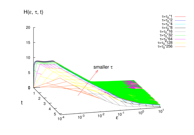
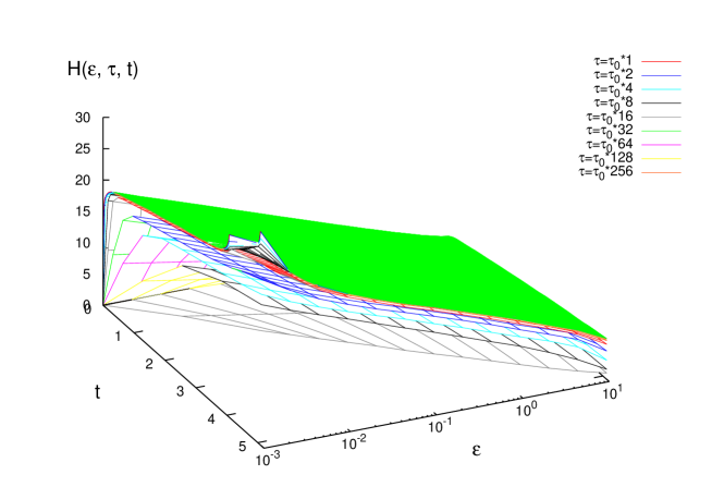
In fig. 1 the joint entropy of the x-coordinate of the Roessler system is given as a function of resolution $\epsilon$, time step length $\tau$ and uncertainty-assessed time $t$. Convergence of the joint entropy for decreasing time step length $\tau$ can be seen. The joint entropy $H$ depends logarithmically on the resolution $\epsilon$, from which the dimension is obtained as a slope according to

$$D_{m}^{(q)}=-\lim_{\epsilon\rightarrow 0}\frac{H_{m}^{(q)}(\epsilon)}{\ln\epsilon}$$ (28)

(schusterjust05 , p.106) with a value as predicted.

It is possible to see in fig. 2 (in comparison with fig. 1 one smaller decade of resolutions is shown) that the z-coordinate of the Roessler attractor carries a different uncertainty for the same values of ($\epsilon,\tau,t$) compared with the x-coordinate. Nevertheless the dimension of the attractor is captured also by the joint entropy of the z-coordinate.

Figure 3: Joint entropy of the x-coordinate of the Roessler system for fixed resolution $\epsilon=10^{-2}$. With respect to time $t$ it is an extended slice of fig. 1 for fixed resolution $\epsilon$.

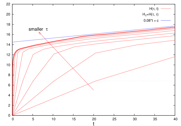
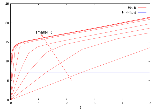
In fig. 3 the slice of fig. 1 for resolution $\epsilon=10^{-2}$ with extended time $t$ is shown. It is found that asymptotically in $t$ the joint uncertainty of the Roessler system increases linearly. The measured slope for smallest $\tau$ in between $t=20$ and $t=40$ is 0.08. It estimates the KS entropy rate

$$h_{KS}=\lim_{\epsilon\rightarrow 0}\lim_{\tau\rightarrow 0}\lim_{t\rightarrow\infty}h(\epsilon,\tau,t)\;.$$ (29)

The deviation from the expected value 0.07 can be found in the fact that still too small $t$ or too large $\epsilon$ are used for the estimation. It can be concluded from the small slope that the uncertainty of the first few points is larger than the uncertainty of a rather long motion in the attractor given the first few points.

Figure 4: Joint entropy of the z-coordinate of the Roessler system for fixed resolution $\epsilon=10^{-2}$. With respect to time $t$ it is an extended slice of fig. 2 for fixed resolution $\epsilon$.

In fig. 4 the slice of fig. 2 for resolution $\epsilon=10^{-2}$ with extended time $t$ is shown. Compared to fig. 3 a much smaller initial uncertainty $H_{1}$ is observed for the z-coordinate. This is understood from the high probability of the z-coordinate to stay at zero. Furthermore in contrast to the x-coordinate a wave-like structure of the joint entropy for smaller time $t$ is observed for the z-coordinate. A non-monotonous entropy rate $h$ as a function of $t$ has to be inferred. This unintuitive signature was robustly reproduced under various parameter values and confidence in this result is caused by the fact that asymptotically for smallest available $\tau$ the slope of 0.08 is found, which serves as a correct estimation of the KS entropy also from the z-coordinate of the Roessler system. Since also (from fig. 2) the dimension of the Roessler dynamics is correctly extractable the result should not be a numerical artefact. Nevertheless it is not expected that this should be true physics in the sense of increasing uncertainty by enlarged conditioning. According to Shannon entropies, for which additional conditioning cannot increase uncertainty, this behaviour is forbidden. A possible explanation of this behaviour can be assigned to effects of Renyi order $q=2$ (cmp. eq. (2)), because in this case it seems unproven that increasing conditioning necessarily reduces the resulting entropy. With this reasoning the example carries the potential of tearing apart the interpretation of uncertainty from $q\neq 1$ - entropies. Another possible explanation that the wave-like structure corresponds to a finite sample effect being responsible for non-ergodicity has to be treated as rather improbable, because also for smallest resolution (largest $\epsilon$) it was not possible to detect a qualitative change in the sense of smoothing of the wave-like structure of the joint entropy under drastical enlargement of the length of the dataset.

With consideration of the fact that the values of $h_{KS}$ and $D$ were estimated for finite large $t$ and finite small $\epsilon$ instead of in the true limit it can be concluded that the same values are obtained from the x- and the z-coordinate of the chaotic Roessler system in the limit cases, in principle in accordance with the theorem of Takens takens81 . On the other hand, it can be clearly seen that for finite time $t$ and finite resolution $\epsilon$ the joint uncertainty is allowed to behave qualitatively different for different observables as the x- and the z-coordinate of the chaotic Roessler system.

Figure 5: Entropy rate as a function of resolution $\epsilon$, uncertainty-assessed time $t$ and varying time discretization interval $\tau$ for the x-coordinate of the Roessler system with parameters for chaotic dynamics. Upper panel: Focus on resolution dependence of divergent behaviour for small time $t$. Lower panel: Focus on larger times $t$ for the Kolmogorov-Sinai entropy rate.

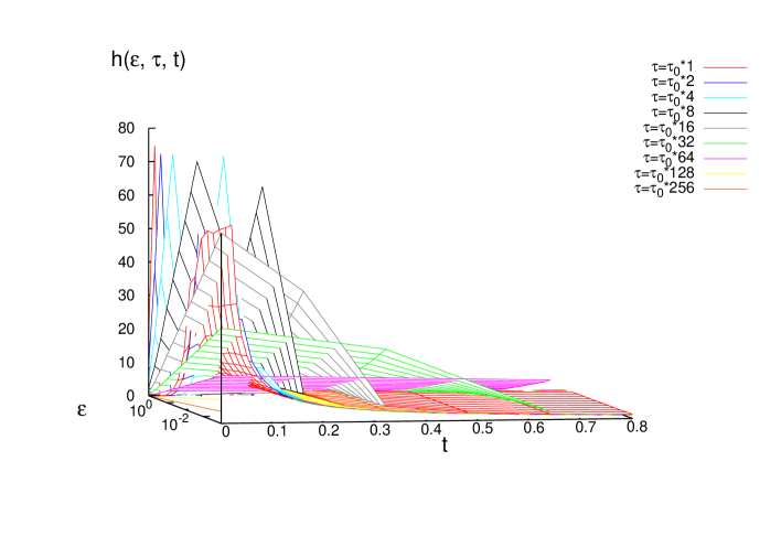
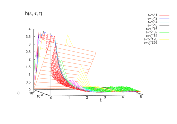
In fig. 5 the entropy rate of the Roessler system is shown. For every $\tau$ the entropy rate as a function of $t$ and $\epsilon$ is represented by a surface. Those surfaces are interleaved for different $\tau$. Depending on the ranges shown along the axes different results become apperent: With the example of the Roessler system even for deterministic dynamics a true divergence of $h(\tau=0,t=0)$ can be observed for sufficiently small $\epsilon$ seen in particular in the upper panel of fig. 5. The trivial argument of eq. (24) already gave a hint for such behaviour. It is possible to see that $h(\epsilon,\tau,t=0)$ for finite $\tau$ increases logarithmically in $\epsilon$ with a slope depending on $\tau$. In the lower panel for larger $t$ the entropy rate indicates a small finite value in the front right corner of the plot, which for sufficiently large $t$ approximates the KS entropy rate.

IV.2 Lorenz system (deterministic chaotic dynamics)

The implemented discretized equations for the Lorenz dynamics are

$$x_{n+1} =x_{n}+\sigma(-x_{n}+y_{n})\Delta t\;,$$

$$y_{n+1} =y_{n}+(-x_{n}z_{n}+rx_{n}-y_{n})\Delta t\;,$$

$$z_{n+1} =z_{n}+(x_{n}y_{n}-bz_{n})\Delta t$$ (30)

with the usual parameters

$$r=28.0\;,\qquad\sigma=10.0\;,\qquad b=\frac{8}{3}\;.$$ (31)

The fractal dimension of the Lorenz attractor is about $D^{(2)}\approx 2.06$ and the largest Lyapunov exponent is $\lambda\approx 0.91$.

Figure 6: Joint entropy of the Lorenz system as a function of the time $t$ and the resolution $\epsilon$ for various $\tau=\tau_{0}\cdot 2^{n}\,;\,n=0,...,8$ ($\tau_{0}=0.01$) for the x-coordinate of the Lorenz dynamics; $3\cdot 10^{6}$ data points.

In fig. 6 the joint entropy of the Lorenz system is shown as a function of the resolution $\epsilon$, time step length $\tau$ and uncertainty-assessed time $t$. As for the Roessler system it is possible to see the convergence of the joint entropy $H$ for decreasing time step length $\tau$ and a logarithmic dependence of the joint entropy on the resolution $\epsilon$ with a slope giving the expected dimension in the limit of infinitesimal small $\epsilon$.

Figure 7: Joint entropy of the Lorenz dynamics for resolution $\epsilon=10^{-2}$ (Slice of fig. 6); $3\cdot 10^{6}$ data points; $\tau_{0}=0.01$.

In fig. 7 a slice of fig. 6 for fixed resolution is shown. An asymptotically linear behaviour in time can be found. The fact, that the slope is steeper than that of the chaotic Roessler attractor of fig. 3 is in accordance with the larger number of nonlinear terms and the known largest Lyapunov exponents. The slightly larger slope compared to the known KS entropy of the Lorenz system can be explained with estimation at rather large $\epsilon$. The appearance of finite sample fluctuations in entropy estimation in fig. 6 for small $\epsilon$, small $\tau$ and large $t$ under the same estimation conditions sooner in the Lorenz-case than in the Roessler-case is in accordance with the enhanced uncertainty $H$ of the Lorenz dynamics.

Furthermore fig. 7 indicates that the joint entropies for different finite $\tau$-values do not coincide for asymptotically large times $t$ even though this cannot finally be proven in a plot for finite $t$. The slopes seem to reach the same value in all cases as already observed in fig. 3 for the x-coordinate of the Roessler dynamics, and hence the estimation of the KS entropy rate is rather independent of the choice of $\tau$, i.e., in the case of deterministic dynamics the limit with respect to $\tau$ in eq. (14) is not so important. On the other hand, the behaviour of $H(\tau=0,t)$ for finite rather small $t$ is better resolved for smaller $\tau$, and this in general is rather important with respect to prediction.

IV.3 Ornstein-Uhlenbeck process (linear stochastic dynamics)

The Ornstein-Uhlenbeck process

$$\dot{X}_{t}=-\alpha X_{t}+\sqrt{D}\,\dot{W}_{t}$$ (32)

can be numerically implemented by its discretisation

$$X_{n+1}=(1-\alpha\Delta t)X_{n}+\sqrt{D}\sqrt{\Delta t}\eta_{n+1}\;,\quad\eta_{n+1}\sim{\mathcal{N}}(0,1)\;\mbox{iid}\;.$$ (33)

Figure 8: Joint entropy of the Ornstein-Uhlenbeck process. Parameters: $\alpha=0.025$; $\tau_{0}=10^{-4}$; 150000 data points.

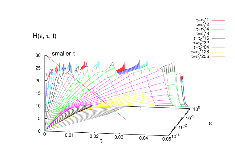
In fig. 8 the numerical analysis of the Ornstein-Uhlenbeck process indicates the non-existence of the limit $\lim_{\tau\rightarrow 0}H(\epsilon,\tau,t)$ for sufficiently small $\epsilon$ and finite $t$ except at $t=0$ for time- and amplitude-continuous stochastic dynamics with continuous trajectories. Whereas in the deterministic case, e.g. for the Lorenz dynamics, the value of the KS entropy rate was approximately seen as a slope at sufficiently small finite $\epsilon$ also for finite $\tau$, in the time- and amplitude-continuous stochastic case the slope of $H$ with respect to $t$ asymptotically in $t$ for sufficiently small finite $\epsilon$ is seen in fig. 8 to be a function of $\tau$. Furthermore it was possible to show numerically that for sufficiently small $\epsilon$ and non-zero finite fixed time $t$ the entropy rate $h(\epsilon,\tau,t>0)$ diverges logarithmically with decreasing $\tau\rightarrow 0$ in the example of Ornstein-Uhlenbeck dynamics. Consistently, fig. 8 supports $h_{KS}=\infty$ for this stochastic dynamics, interestingly already from the $\tau$-behaviour. It should be mentioned here that for $\tau>0$ eq. (20) can be seen as a naturally given regularization of the unavailable eq. (22) in the stochastic case.

The author is aware of the fact that the result concerning the $\tau$-dependence contradicts (gaspard93 , p.322) according to which processes with continuous realizations are said to have $\tau$-independent $(\epsilon,\tau)$-entropies $h(\epsilon,\tau)$ per unit time, which corresponds to the suggestion of finite $\lim_{\tau\rightarrow 0}H(\epsilon,\tau,t)$. The argument for this behaviour was essentially that for finite $\epsilon$ a finite crossing time of underlying boxes of the partition leads to finite uncertainty for continuous trajectories (gaspard93 , p.317). On the other hand, an explanation for the numerically found behaviour in fig. 8 could be that infinite uncertainty arises from the trajectories close to the border of boxes of partitioning, where in the limit of $\tau\to 0$ infinitely often moving back and forth between boxes in finite time $t$ is in principle possible for the Ornstein-Uhlenbeck process. This would create an infinite and hence dominant contribution for an averaged uncertainty calculation.

Figure 9: The same plot as in fig. 8 from another point of view.

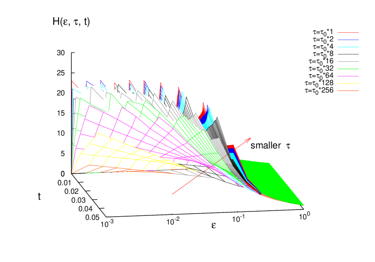
From fig. 9 it is obtained that in the transition regime of large $\epsilon$ the behaviour of non-existing $\lim_{\tau\rightarrow 0}H(\epsilon,\tau,t)$ is suppressed. The plots do not allow for the decision of the question if the transition from finite to infinite occurs at the resolution of the size of the system or at a smaller value for $\epsilon$. According to eq. (28) fig. 9 yields finite dimensions for finite $\tau$ increasing in $t$ for stochastic dynamics, even though the limit $\epsilon\rightarrow 0$ can of course not be seen. In the limit of $\tau\rightarrow 0$, what is effectively like the limit of $m\rightarrow\infty$, fig. 9 suggests an infinite dimension for stochastic dynamics.

The results of this section are qualitatively robust against changes of the parameter $\alpha$ of the Ornstein-Uhlenbeck process and hence qualitatively robust against changes of the autocorrelation of the process.

V Conclusion

The central objects of investigation in this paper are the entropy $H^{(q)}(\epsilon,\tau,t)$ and the entropy rate $h^{(q)}(\epsilon,\tau,t)$ as a function of the resolution $\epsilon$, the time discretization step length $\tau$ and the uncertainty-assessed time $t$ with numerical access to the case of Renyi order $q=2$. Special focus is laid on the analysis of the behaviour of these quantities for varying $\tau$ and especially on the time-continuous limit $\tau\rightarrow 0$ while $t$ is kept finite. In case of existence, in the time-continuous limit the entropy rates can be understood as usual time-derivatives of entropies. However, for finite $\tau$, in consequence of the explicit $\tau$-dependence of entropies, discrepancies from the usual quotient of differences are present.

Numerically the analysis of time- and space-continuous dynamics was carried out with the Roessler and Lorenz system for the deterministic case and with the Ornstein-Uhlenbeck process for the stochastic case. Qualitative discrepancies of deterministic and stochastic dynamics were found. In the deterministic case the uncertainty $H(\epsilon,\tau=0,t)$ is finite for all finite $\epsilon$ and $t$. The entropy rate $h(\epsilon,\tau=0,t)$ becomes constant for large $t$ and sufficiently small $\epsilon$. In the stochastic case the uncertainty $H(\epsilon,\tau=0,t)$ is infinite for all $t>0$ if $\epsilon$ is below some threshold. Only for $\epsilon$ above the threshold it is finite and then effectively like in the deterministic case. The stochastic result is qualitatively independent of the value of the width of the input noise as long as the width is not exactly zero, corresponding to determinism and introducing the qualitative change. This behaviour of entropies in the limit $\tau\rightarrow 0$ seems to offer a new possibility for distinction of chaos and noise (see also cencini00 ).

The convergence of $H$ in the limit $\tau\rightarrow 0$ in the deterministic case can be interpreted as a saturation of the gain from higher sampling rates, such that a threshold sampling rate can be postulated, above which almost nothing more can be learned, i.e., in the deterministic case the continuous limit can be well approximated by discrete sampling with sufficiently high sampling rate. A criterion for an optimal sampling rate could be formulated.

In the limit case $\epsilon\rightarrow 0$ the partial derivative of the joint entropy $H$ with respect to $\ln\epsilon$ yields (minus) the dimension and if furthermore the limit $t\rightarrow\infty$ is carried out, the partial derivative of $H$ with respect to $t$ yields the KS entropy rate. All information concerning entropy rates (including the KS entropy rate) and dimensions of the dynamics can be extracted from one single plot of $H^{(q)}(\epsilon,\tau,t)$. In the deterministic case known values were verified in examples. For time- and amplitude-continuous stochastic dynamics it was seen that the partial derivative of $H$ with respect to minus $\ln\epsilon$ becomes infinite for $t\to\infty$ or $\tau\to 0$ and the partial derivative of H with respect to $t$ becomes infinite for $\epsilon\to 0$ or $\tau\to 0$.

According to usual rules the total differential of the joint entropy $H$ can be written as

$$dH=\frac{\partial H}{\partial t}\,dt+\frac{\partial H}{\partial\ln\epsilon}\,d\ln\epsilon\;.$$ (34)

For sufficiently small $\epsilon$ and sufficiently large $t$ this becomes

$$dH=h_{KS}\,dt-D\,d\ln\epsilon\;.$$ (35)

It is possible to see that directional derivatives of $H$ in general mix the properties of dimension and entropy rate. For integral quantities $H(\epsilon,t)\approx h_{KS}\,t-D\log\epsilon+\operatorname{const}$   was suggested in (grassberger91 , p.529), from which eq. (35) can be derived, but a prescription for the calculation of the constant is not given. Since eq. (35) avoids the offset problems it is a slightly reduced and hence preferable representation of the relationship of the involved quantities.

Concerning the limit cases $t\to\infty$ and $\epsilon\to 0$ with the determination of dynamical invariants, which is discussed in the literature, e.g. see (farmer82 , p.1321), the time-continuous case treated in this paper gives a new unified representation of singly known results. On the other hand, at least of the same importance, the case of finite time $t$ is of strong interest, if questions concerning optimal finite time conditioning with respect to prediction are addressed. A finite resolution $\epsilon$ is needed for optimality of local prediction methods. With finite $t$ and $\epsilon$, the limit $\tau\to 0$ is of interest for the determination of the informational characteristic of the dynamics.

A non-monotonous entropy rate for Renyi order $q=2$, i.e., a conditional entropy, which does not monotonously decrease in the length of conditioning, is numerically found for the z-coordinate of the Roessler system in fig. 4. This could be interpreted as a hint for problems of the interpretation of uncertainty for entropies with $q\neq 1$ in maximal generality.

References

- (1) T.M. Cover and J.A. Thomas, Elements of Information Theory, Wiley, New York (1991).
- (2) A. Renyi, On measures of entropy and information, Proc. IV Berkeley Symposium Math. Statist. and Prob., University California Press, 547-561 (1961).
- (3) P. Grassberger and I. Procaccia, Estimation of the Kolmogorov entropy from a chaotic signal, Phys. Rev. A 28 (4) 2591-2593 (1983).
- (4) H. Kantz and T. Schreiber, Nonlinear Time Series Analysis, Cambridge University Press, second edition (2004).
- (5) J.P. Crutchfield and D.P. Feldman; Regularities unseen, randomness observed: Levels of entropy convergence, Chaos 13 (1) 25-54 (2003).
- (6) P. Gaspard and X.-J. Wang; Noise, chaos and (, )-entropy per unit time, Phys. Rep. 235 (6) 291-343 (1993).
- (7) M. Cencini, M. Falcioni, E. Olbrich, H. Kantz and A. Vulpiani; Chaos or noise: Difficulties of a distinction, Phys. Rev. E 62 (1) 427-437 (2000).
- (8) D. Holstein, Generalized Markov Approximations from information theory and consequences for prediction, Dissertation, Wuppertal (2007).
- (9) H.G. Schuster and W. Just; Deterministic Chaos: An Introduction, Wiley, Weinheim, fourth edition (2005).
- (10) F. Takens; Detecting strange attractors in turbulence, Lecture Notes in Mathematics 898, Springer, New York (1981).
- (11) P. Grassberger, T. Schreiber, and C. Schaffrath; Nonlinear time sequence analysis, Int. Journ. of Bifurcation and Chaos 1 (3) 521-547 (1991).
- (12) J.D. Farmer; Information Dimension and the Probabilistic Structure of Chaos, Z. Naturforsch. 37a 1304-1325 (1982).