Large-scale dynamos in turbulent convection with shear

Abstract

Aims. To study the existence of large-scale convective dynamos under the influence of shear and rotation.

Methods. Three-dimensional numerical simulations of penetrative compressible convection with uniform horizontal shear are used to study dynamo action and the generation of large-scale magnetic fields. We consider cases where the magnetic Reynolds number is either marginal or moderately supercritical with respect to small-scale dynamo action in the absence of shear and rotation. Our magnetic Reynolds number is based on the wavenumber of the depth of the convectively unstable layer. The effects of magnetic helicity fluxes are studied by comparing results for the magnetic field with open and closed boundaries.

Results. Without shear no large-scale dynamos are found even if the ingredients necessary for the $\alpha$-effect (rotation and stratification) are present in the system. When uniform horizontal shear is added, a large-scale magnetic field develops, provided the boundaries are open. In this case the mean magnetic field contains a significant fraction of the total field. For those runs where the magnetic Reynolds number is between 60 and 250, an additional small-scale dynamo is expected to be excited, but the field distribution is found to be similar to cases with smaller magnetic Reynolds number where the small-scale dynamo is not excited. In the case of closed (perfectly conducting) boundaries, magnetic helicity fluxes are suppressed and no large-scale fields are found. Similarly, poor large-scale field development is seen when vertical shear is used in combination with periodic boundary conditions in the horizontal directions. If, however, open (normal-field) boundary conditions are used in the $x$-direction, a large-scale field develops. These results support the notion that shear not only helps to generate the field, but it also plays a crucial role in driving magnetic helicity fluxes out of the system along the isocontours of shear, thereby allowing efficient dynamo action.

1 Introduction

It is evident that the Sun possesses a large-scale magnetic field. The most likely origin of this field is a hydromagnetic dynamo working within or somewhat below the turbulent convection zone (e.g. Ossendrijver 2003). The solar dynamo is generally thought to rely on large-scale shear to produce toroidal magnetic field from poloidal field and a process called the $\alpha$-effect which produces poloidal field from toroidal field. In the turbulent mean-field dynamo picture an $\alpha$-effect can arise due to helical motions in a stratified fluid in the presence of either rotation or shear, or both (Rogachevskii & Kleeorin RogaKle2003 (2003); Rüdiger & Kitchatinov RueKit2006 (2006); Rädler & Stepanov RaedStep2006 (2006)). Other candidates for regenerating large-scale magnetic fields in shearing turbulence include the incoherent $\alpha\Omega$-effect (Vishniac & Brandenburg VishBran1997 (1997); Proctor Proctor2007 (2007)) and the shear–current effect (Rogachevskii & Kleeorin RogaKle2003 (2003, 2004)).

Numerical simulations of convection have been used to study dynamo action in local (e.g. Cattaneo & Hughes CattHugh2006 (2006); Tobias et al. Tobiasea2008 (2008)) and global (e.g. Brun et al. BMT04 (2004), Browning et al. Browning_etal06 (2006), Brown et al. Brown_etal07 (2007)) settings. So far, however, with the exception of the last two papers, these models have had a hard time generating appreciable large-scale magnetic fields, although all the ingredients such as rotation and stratification necessary for an $\alpha$-effect to occur have been present. Possible reasons for the lack of large-scale dynamo action in the numerical models is arguably the lack of scale separation between the energy carrying scale and the scale of the domain and the absence of large-scale shear in the system. In stratified convection, the lack of sufficient scale separation is difficult to tackle due to the prohibitive computational challenges involved when trying to cover many more vertical scale heights in the domain. Adding shear, however, is easier to accomplish, which is one of the principal aims of the present paper.

An additional point concerning large-scale dynamo action in turbulent convection is the possibility of catastrophic quenching due to small-scale magnetic fields. It has long been argued that small-scale fields cause catastrophic quenching of the large-scale dynamo (e.g. Vainshtein & Cattaneo VainCatt1992 (1992)). This sort of quenching, however, only occurs in specific circumstances, i.e. when there is no magnetic helicity flux out of the domain. This behaviour can be understood in terms of magnetic helicity (Brandenburg & Subramanian 2005a ) which is a conserved quantity in ideal MHD. If magnetic diffusivity is finite, the magnetic helicity can only change diffusively under the aforementioned special circumstances that lead to resistively slow saturation of the large-scale field.

If, however, magnetic helicity is driven out of the domain, catastrophic quenching can be alleviated and the large-scale dynamo is expected to saturate near equipartition field strengths. A promising mechanism capable of driving magnetic helicity fluxes was introduced by Vishniac & Cho (VishCho2001 (2001)), who found that in the presence of shear the flux follows isocontours of constant velocity (Brandenburg & Subramanian 2005b ; Subramanian & Brandenburg SB06 (2006)). We expect that this shear-driven magnetic helicity flux is of crucial importance for large-scale dynamo action.

The remainder of the paper is organised as follows: the numerical model is described in Sect. 2, and the results and conclusions are presented in Sects. 3 and 4, respectively.

2 The model

Our model setup is similar to that used by Brandenburg et al. (Brandea1996 (1996)), Ossendrijver et al. (Osseea2001 (2001)) and Käpylä et al. (Kaepylaeea2004 (2004), Kaepylaeea2006 (2006)). A rectangular portion of a star is modelled by a box situated at colatitude $\theta$. The dimensions of the computational domain are $(L_{x},L_{y},L_{z})=(4,4,2)d$, where $d$ is the depth of the convectively unstable layer, which is also used as the unit of length. The box is divided into three layers, an upper cooling layer, a convectively unstable layer, and a stable overshoot layer (see below). The following set of equations for compressible magnetohydrodynamics is being solved:

$$\frac{\mathcal{D}\bm{A}}{\mathcal{D}t}=-SA_{y}\hat{\bm{x}}-(\bm{\nabla}\bm{U})^{\rm T}\bm{A}-\mu_{0}\eta{\bm{J}},$$ (1)

$$\frac{\mathcal{D}\ln\rho}{\mathcal{D}t}=-\@vec{\nabla}\cdot{\bm{U}},$$ (2)

$$\frac{\mathcal{D}\bm{U}}{\mathcal{D}t}=-SU_{x}\bm{\hat{y}}-\frac{1}{\rho}{\bm{\nabla}}p+{\bm{g}}-2\bm{\Omega}\times\bm{U}+\frac{1}{\rho}\bm{J}\times{\bm{B}}+\frac{1}{\rho}\bm{\nabla}\cdot 2\nu\rho\mbox{\boldmath${\sf S}$},$$ (3)

$$\frac{\mathcal{D}e}{\mathcal{D}t}=-\frac{p}{\rho}\@vec{\nabla}\cdot{\bm{U}}+\frac{1}{\rho}\bm{\nabla}\cdot K\bm{\nabla}T+2\nu\mbox{\boldmath${\sf S}$}^{2}+\frac{\mu_{0}\eta}{\rho}\bm{J}^{2}-\frac{e\!-\!e_{0}}{\tau(z)},$$ (4)

where $\mathcal{D}/\mathcal{D}t=\partial/\partial t+(\bm{U}+\overline{\bm{U}}_{0})\cdot\bm{\nabla}$, and $\overline{\bm{U}}_{0}=(0,Sx,0)$ is the imposed large-scale shear flow. $\bm{A}$ is the magnetic vector potential, $\bm{B}=\bm{\nabla}\times\bm{A}$ the magnetic field, and $\bm{J}=\bm{\nabla}\times\bm{B}/\mu_{0}$ is the current density, $\mu_{0}$ is the magnetic permeability, $\eta$ and $\nu$ are the magnetic diffusivity and kinematic viscosity, respectively, $K$ is the heat conductivity, $\rho$ the density, $\bm{U}$ the velocity, $\bm{g}=-g\hat{\bm{z}}$ the gravitational acceleration, and $\bm{\Omega}=\Omega_{0}(-\sin\theta,0,\cos\theta)$ the rotation vector. The fluid obeys an ideal gas law $p=\rho e(\gamma-1)$, where $p$ and $e$ are the pressure and internal energy, respectively, and $\gamma=c_{\rm P}/c_{\rm V}=5/3$ is the ratio of specific heats at constant pressure and volume, respectively. The specific internal energy per unit mass is related to the temperature via $e=c_{\rm V}T$. The rate of strain tensor ${\sf S}$ is given by

$${\sf S}_{ij}={\textstyle{1\over 2}}(U_{i,j}+U_{j,i})-{\textstyle{1\over 3}}\delta_{ij}\@vec{\nabla}\cdot\bm{U}.$$ (5)

The last term of Eq. (4) describes cooling at the top of the domain. Here, $\tau(z)$ is a cooling time which has a profile smoothly connecting the upper cooling layer and the convectively unstable layer below, where $\tau\to\infty$.

The positions of the bottom of the box, bottom and top of the convectively unstable layer, and the top of the box, respectively, are given by $(z_{1},z_{2},z_{3},z_{4})=(-0.85,0,1,1.15)d$. Initially the stratification is piecewise polytropic with polytropic indices $(m_{1},m_{2},m_{3})=(3,1,1)$, which leads to a convectively unstable layer above a stable layer at the bottom of the domain and an isothermal cooling layer at the top. All simulations with rotation use $\theta=0\degr$ corresponding to the north pole.

2.1 Nondimensional units and parameters

Non-dimensional quantities are obtained by setting

$$d=g=\rho_{0}=c_{\rm P}=\mu_{0}=1\;,$$ (6)

where $\rho_{0}$ is the initial density at $z_{2}$. The units of length, time, velocity, density, entropy, and magnetic field are

$$[x]=d\;,\;\;[t]=\sqrt{d/g}\;,\;\;[U]=\sqrt{dg}\;,\;\;[\rho]=\rho_{0}\;,\;\;$$

$$[s]=c_{\rm P}\;,\;\;[B]=\sqrt{dg\rho_{0}\mu_{0}}\;.$$ (7)

We define the fluid and magnetic Prandtl numbers and the Rayleigh number as

$${\rm Pr}=\frac{\nu}{\chi_{0}}\;,\;\;{\rm Pm}=\frac{\nu}{\eta}\;,\;\;{\rm Ra}=\frac{gd^{4}}{\nu\chi_{0}}\bigg{(}-\frac{1}{c_{\rm P}}\frac{{\rm d}s}{{\rm d}z}\bigg{)}_{0}\;,$$ (8)

where $\chi_{0}=K/(\rho_{\rm m}c_{\rm P})$ is the thermal diffusivity, and $\rho_{\rm m}$ is the density in the middle of the unstable layer. The entropy gradient, measured in the middle of the convectively unstable layer in the non-convecting hydrostatic state, is given by

$$\bigg{(}-\frac{1}{c_{\rm P}}\frac{{\rm d}s}{{\rm d}z}\bigg{)}_{0}=\frac{\nabla-\nabla_{\rm ad}}{H_{\rm P}}\;,$$ (9)

where $\nabla-\nabla_{\rm ad}$ is the superadiabatic temperature gradient with $\nabla_{\rm ad}=1-1/\gamma$, $\nabla=(\partial\ln T/\partial\ln p)_{z_{\rm m}}$, where $z_{\rm m}=z_{3}-z_{2}$, and $H_{\rm P}$ being the pressure scale height (Brandenburg et al. Brandea2005 (2005)). The amount of stratification is determined by the parameter $\xi_{0}=(\gamma-1)e_{0}/(gd)$, which is the pressure scale height at the top of the domain normalized by the depth of the unstable layer. We use in all cases $\xi_{0}=0.3$, which results in a density contrast of about 23. We define the magnetic Reynolds number via

$${\rm Rm}=\frac{u_{\rm rms}}{\eta k_{\rm f}}\;,$$ (10)

where $k_{\rm f}=2\pi/d$ is assumed as a reasonable estimate for the wavenumber of the energy-carrying eddies. Note that our definition of ${\rm Rm}$ is smaller than the usually adopted one by a factor $2\pi$. The amount of shear and rotation is quantified by

$${\rm Sh}=\frac{S}{u_{\rm rms}k_{\rm f}}\;,\quad{\rm Co}=\frac{2\,\Omega_{0}}{u_{\rm rms}k_{\rm f}}\;.$$ (11)

The denominators in Eq. (11) give an estimate of the convective turnover time. The equipartition magnetic field is defined by

$$B_{\rm eq}\equiv\langle\mu_{0}\rho\bm{U}^{2}\rangle^{1/2},$$ (12)

where the angular brackets denote volume averaging.

2.2 Boundary conditions

Table 1: Summary of the runs. The numbers are given for the saturated state of the dynamo (except for Run E1, which was not run to saturation). Runs D and D3 are the same model. Here, $\mbox{Ma}=u_{\rm rms}/(gd)^{1/2}$, $\tilde{B}_{\rm rms}\equiv B_{\rm rms}/B_{\rm eq}$, $\langle\tilde{\overline{B}}_{y}^{2}\rangle^{1/2}=\langle\overline{B}_{y}^{2}\rangle^{1/2}/B_{\rm rms}$, and $Q^{-1}=\langle\overline{B}_{x}^{2}\rangle^{1/2}/\langle\overline{B}_{y}^{2}\rangle^{1/2}$. The last column gives the magnetic field boundary condition at the $z$-boundaries, except for the last two lines where the $x$-boundary condition is given. ${\rm Pm}=5$ in all models except D6 where ${\rm Pm}=10$.

$$\begin{array}[]{p{0.035\linewidth}cccccccccccc}\hline\cr\vskip 3.0pt plus 1.0pt minus 1.0pt\cr Run&$grid$&${\rm Pr}$&${\rm Ra}$&$Rm$&{\rm Sh}&{\rm Co}&\mbox{Ma}&\tilde{B}_{\rm rms}&\langle\tilde{\overline{B}}_{y}^{2}\rangle^{1/2}&Q^{-1}&$BC$\\ \hline\cr A&256^{3}&0.69&6.1\cdot 10^{5}&70&0&0&0.044&0.19&0.05&0.90&$vf$\\ B&256^{3}&0.69&6.1\cdot 10^{5}&61&0&0.42&0.038&0.31&0.05&0.83&$vf$\\ C&256^{3}&0.69&6.1\cdot 10^{5}&74&-0.17&0&0.046&1.09&0.55&0.11&$vf$\\ C'&256^{3}&0.69&6.1\cdot 10^{5}&92&-0.14&0&0.058&0.37&0.22&0.31&$pc$\\ D&256^{3}&0.69&6.1\cdot 10^{5}&56&-0.23&0.46&0.036&1.41&0.61&0.15&$vf$\\ \hline\cr D1&64^{3}&2.74&1.5\cdot 10^{5}&11&-0.28&0.56&0.028&1.72&0.82&0.13&$vf$\\ D2&128^{3}&1.37&3.1\cdot 10^{5}&25&-0.25&0.50&0.032&1.45&0.67&0.17&$vf$\\ D3&256^{3}&0.69&6.1\cdot 10^{5}&56&-0.23&0.46&0.035&1.41&0.61&0.15&$vf$\\ D4&384^{3}&0.48&8.8\cdot 10^{5}&83&-0.22&0.44&0.036&1.37&0.58&0.16&$vf$\\ D5&512^{3}&0.34&1.2\cdot 10^{6}&121&-0.21&0.42&0.038&1.52&0.53&0.19&$vf$\\ D6&512^{3}&0.34&1.2\cdot 10^{6}&250&-0.20&0.40&0.039&1.42&0.51&0.20&$vf$\\ \hline\cr D2d&128^{2}\times 192&1.37&3.1\cdot 10^{5}&23&-0.27&0.54&0.029&2.44&0.89&0.08&$vf$\\ D2w&256^{2}\times 128&1.37&3.1\cdot 10^{5}&26&-0.24&0.48&0.033&1.56&0.68&0.15&$vf$\\ \hline\cr E1&128^{3}&1.37&3.1\cdot 10^{5}&42&-0.03&0&0.052&0.03&0.08&0.64&$vf$\\ E2&128^{3}&1.37&3.1\cdot 10^{5}&33&-0.08&0&0.041&0.83&0.48&0.19&$vf$\\ E3&128^{3}&1.37&3.1\cdot 10^{5}&30&-0.15&0&0.038&1.08&0.63&0.13&$vf$\\ E4&128^{3}&1.37&3.1\cdot 10^{5}&29&-0.22&0&0.036&1.14&0.74&0.09&$vf$\\ E5&128^{3}&1.37&3.1\cdot 10^{5}&41&-0.22&0&0.051&1.01&0.55&0.14&$vf$\\ \hline\cr VSA&128^{3}&1.37&3.1\cdot 10^{5}&46&-0.27&0&0.058&0.27&0.07&0.90&$p$\\ VSA'&128^{3}&1.37&3.1\cdot 10^{5}&45&-0.28&0&0.056&0.31&0.39&0.17&$nf$\\ \hline\cr\end{array}$$

Stress-free boundary conditions are used for the velocity,

$$U_{x,z}=U_{y,z}=U_{z}=0,$$ (13)

and either vertical field or perfect conductor conditions for the magnetic field, i.e.

$$B_{x}=B_{y} = 0,\;\;{\rm(Vertical\;Field)}$$ (14)

$$B_{x,z}=B_{y,z}=B_{z} = 0,\;\;{\rm(Perfect\;Conductor)}$$ (15)

respectively. We may think of them as open and closed boundaries, respectively, because they either do or they do not permit a magnetic helicity flux. In the $y$ and $x$ directions we use periodic and shearing-periodic boundary conditions, respectively. The simulations were made with the Pencil Code, which uses sixth-order explicit finite differences in space and third order accurate time stepping method. Resolutions of up to $512^{3}$ mesh points were used.

Figure 1: Vertical velocity in the middle of the convectively unstable layer of Runs A–D (from left to right) during the kinematic stage of the simulations [upper row of panels, $t=200\,(d/g)^{1/2}$ corresponding to $tu_{\rm rms}k_{\rm f}\approx 50$] and the saturated state [lower row, $t=2000\,(d/g)^{1/2}$ or $tu_{\rm rms}k_{\rm f}\approx 500$].

3 Results

3.1 Description of the hydrodynamic state

The hydrodynamics of local rotating convection simulations similar to ours has been discussed previously in the literature (e.g. Brandenburg et al. Brandea1996 (1996); Käpylä et al. Kaepylaeea2004 (2004)). However, the imposed shear flow used in the present runs is a new element. Thus it is interesting to consider the differences to the cases where it is absent. We consider four representative runs where physical ingredients are added individually in order to see their respective effects. In Run A neither rotation nor shear are present, whereas in Runs B and C only rotation and only shear are applied, respectively. In Run D both shear and rotation are used (see Table 1 for details).

All our runs start with a weak magnetic field ($10^{-5}$ times the equipartition value). For Runs A to D it takes about 200 turnover times for this field to grow to values such that it affects the flow, so we consider this as the kinematic stage of the simulation. We use this time span to characterize the basic hydrodynamic state.

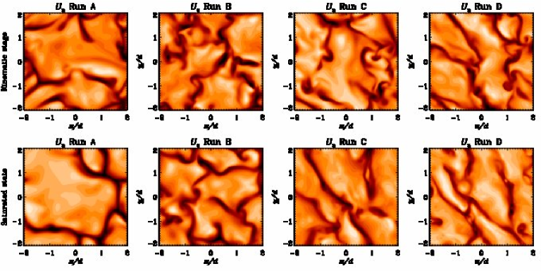
The upper row of panels in Fig. 1 shows the vertical velocity in the middle of the convectively unstable layer for Runs A to D. In the cases without shear (Runs A and B), the convective pattern is dominated by large cells which are isotropic in the horizontal plane. In the case with rotation (Run B), the downflows at the vertices of convective cells tend to exhibit vortical structures, contributing to net helicity. When shear is added the convective cells are slightly elongated along the $y$ direction, which is the direction of the imposed large-scale flow.

The horizontally averaged root mean square velocity shows a very similar profile in all models, i.e. peaking near the top of the convectively unstable layer and decreasing towards the base of the layer, see Fig. 2. The runs without shear are close to each other, with somewhat smaller velocities in the case with rotation (Run B). When a horizontal shear flow is added, the rms velocity is somewhat larger, but in Run D $u_{\rm rms}$ decreases again. The shear flow itself does not contribute to the definition of the rms velocity.

The left panel of Fig. 3 shows the horizontal averages of kinetic helicity density for Runs A to D averaged over the initial kinematic stage of the simulations. In the case without rotation or shear (Run A) very little net helicity is produced. Adding rotation corresponding to the north pole ($\@vec{g}\cdot\@vec{\Omega}<0$; Run B) produces significant negative helicity within the convection zone, suggestive of a positive $\alpha$-effect. In the case with only shear ($S<0$, so that $\@vec{g}\cdot\@vec{\nabla}\times\overline{\@vec{U}}>0$; Run C) the helicity profile is similar to Run B, but of opposite sign and roughly half the magnitude. If both rotation and shear are present, as in Run D, the sign and profile are very similar to Run B, but the magnitude is smaller by approximately a factor of two. This suggests that there is partial cancellation of the two effects.

Figure 2: Horizontal averages of the rms velocity in the kinematic (left panel) and saturated states (right panel) for Runs A to D. Linestyles are indicated in the legend in the left panel. The vertical lines at $z=(0,1)d$ denote the base and top of the convectively unstable layer, respectively.

Figure 3: Horizontal averages of kinetic helicity in the kinematic (left panel) and saturated states (right panel) for Runs A to D. Linestyles are indicated in the legend in the left panel.

Figure 4: Power spectra of velocity from the middle of the convectively unstable layer from the kinematic (left panel) and saturated states (right panel). Linestyles as in Fig. 2. The straight lines with a slope of $-5/3$ are given for comparison.

In the late stages of the simulations when the magnetic field has saturated the convective pattern does not change significantly in the cases without shear (see the lower row of Fig. 1). In Runs C and D, there seems to be a larger change, i.e. clearer elongation of cells along the $y$ direction, possibly due to the strong large-scale magnetic field that develops in those cases. Figures 2 and 3 show that velocity and helicity decrease somewhat in comparison to the hydrodynamic state in all cases except Run D where the helicity seems to increase. Part of this change can be attributed to the fact that some of the runs were not yet fully relaxed during the kinematic phase and that they are still undergoing a slow thermal adjustment, especially in the cases without shear. However, in Runs C and D where the dynamo grows to super-equipartition strengths, the magnetic field is likely to be responsible for much of the change.

In the absence of shear the spectra are similar to those published previously (e.g. Brandenburg et al. Brandea1996 (1996)), but with shear we should really only look at one-dimensional spectra in the streamwise direction, because this is the only periodic direction. In the kinematic stage little difference is seen between the four runs (see the left panel of Fig. 4). However, in the saturated state the spectra for the shearing runs are steeper than for the non-shearing runs. This may indicate the development of large-scale ordered velocity structures.

3.2 Excitation of dynamo action

We consider first the effects of shear and rotation on the dynamo. In Fig. 5 we show the resulting growth of the rms magnetic field for ${\rm Rm}=56\ldots 74$ and ${\rm Pm}=5$ for Runs A to D introduced in the previous section. The slowest growth occurs in Run A with no rotation and no shear ($\lambda=0.016\,u_{\rm rms}k_{\rm f}$). Adding rotation (Run B; ${\rm Co}=0.42$) almost doubles the growth rate ($\lambda=0.03\,u_{\rm rms}k_{\rm f}$), and the saturation field strength of the horizontally averaged field is somewhat higher: $\overline{B}\approx 0.4\,B_{\rm eq}$. Next, adding shear (Run C) raises the growth rate further and, more importantly, it raises the saturation field strength by a factor of about 3 ($\overline{B}\approx 1.1\,B_{\rm eq}$). Again, adding rotation (Run D) increases the growth rate further ($\lambda=0.04\,u_{\rm rms}k_{\rm f}$), and increases the saturation level by almost fifty per cent. In the absence of shear and rotation the critical Reynolds number is $\approx 30$ for open (vertical field) boundary conditions (see Sect. 3.6 for more details on the effects of boundary conditions). If shear is included, the dynamo is excited already at ${\rm Rm}\approx 5$.

We note that in the kinematic phase the mean and total fields have the same growth rate. The two begin to depart from each other only in the saturation phase which is achieved more quickly for the small-scale field. This behaviour is reminiscent of dynamos where the saturation of the large-scale field is controlled by magnetic helicity evolution (Blackman & Brandenburg BB02 (2002)).

Figure 5: Growth of the total rms magnetic field from four runs, which were performed without shear or rotation (solid line, Run A), with only rotation (dashed, Run B), only shear (dash-dotted, Run C), and with shear and rotation (triple-dot-dashed, Run D), respectively. ${\rm Pm}=5$, $\rm Rm\approx 60\ldots 90$, and grid resolution $256^{3}$ in all runs, see also Table 1.

Figure 6: Horizontally averaged magnetic fields $\overline{B}_{x}$ (upper panel) and $\overline{B}_{y}$ (lower panel), normalized by the volume average of $B_{\rm eq}$, as functions of time and $z$ for Run D5 with ${\rm Rm}=121$, ${\rm Sh}=-0.21$, and ${\rm Co}=0.42$. The dotted white lines show top ($z=d$) and bottom ($z=0$) of the convection zone.

Figure 7: Same as Fig. 6, but for Run C with ${\rm Rm}=74$, ${\rm Sh}=-0.17$, and ${\rm Co}=0$.

Figure 8: Rms-values of the total magnetic field (solid line), the mean field $\overline{B}_{\rm rms}=\langle\overline{B}_{x}^{2}+\overline{B}_{y}^{2}\rangle^{1/2}$ (dashed line) and fluctuating field with $b_{\rm rms}^{2}=B_{\rm rms}^{2}-\overline{B}^{2}_{\rm rms}$ (dot-dashed line) for Run D5.

Figure 9: Snapshots of $B_{y}$ in the early phase (left: $t=200\,(d/g)^{1/2}$, corresponding to $tu_{\rm rms}k_{\rm f}\approx 50$) and saturated phase (right: $t=1500\,(d/g)^{1/2}$, or $tu_{\rm rms}k_{\rm f}\approx 360$) for Run D5. The sides of the box show the periphery of the domain whereas the top and bottom slices show $B_{y}$ at vertical heights $z=d$ and $z=0$, respectively. See also http://www.helsinki.fi/$\sim$kapyla/movies.html

3.3 Large-scale magnetic fields

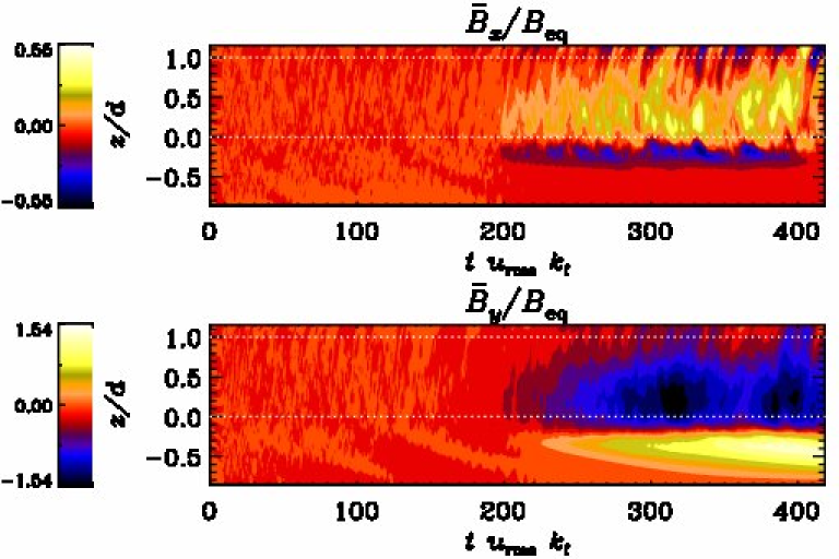
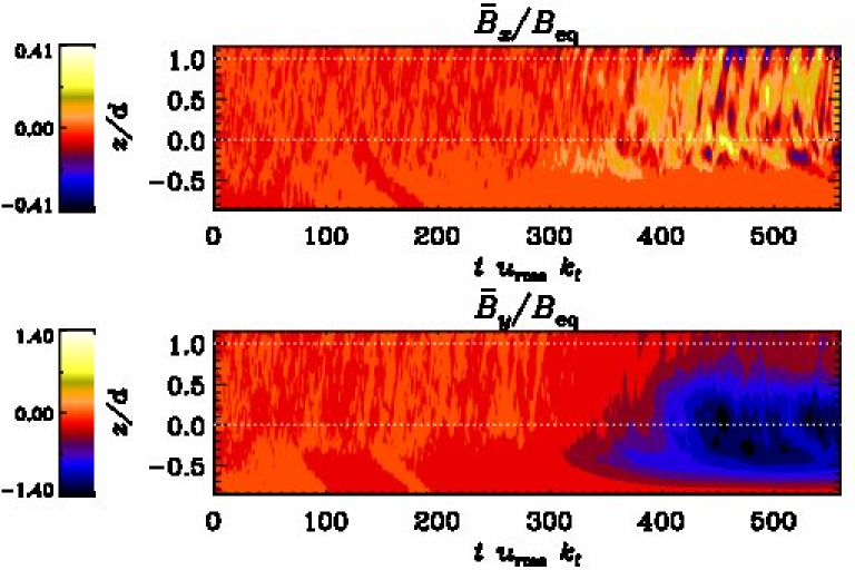
Adding a large-scale shear flow not only makes the dynamo easier to excite, it also helps the generation of large-scale magnetic fields and, most importantly, it is expected to drive magnetic helicity fluxes along lines of constant shear (Vishniac & Cho VishCho2001 (2001); Subramanian & Brandenburg SB06 (2006)). A representative solution from Run D5 with ${\rm Rm}=121$, ${\rm Sh}=-0.21$, and ${\rm Co}=0.42$ is shown in Fig. 6. Note that in runs with rotation the large-scale field has opposite sign in the overshoot layer and the convection zone, whereas in models with only shear the field has the same sign everywhere; see Fig. 7.

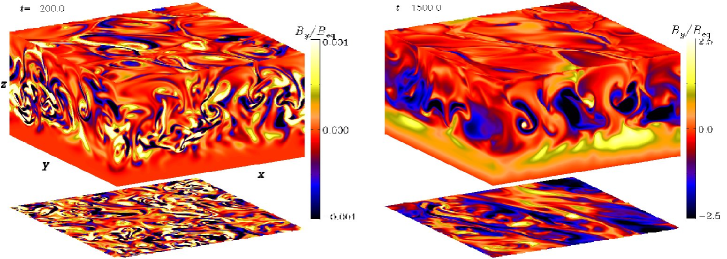
In all cases the magnetic energy grows exponentially from a weak small-scale seed magnetic field. Generally the small-scale dynamo saturates first and a large-scale field develops later; see Fig. 8 for representative results from Run D5. Figure 9 shows that during this process the magnetic field changes from a filamentary field to a more diffuse one. This behaviour has also been seen in simulations of forced turbulence with shear and open boundaries (Brandenburg 2005). The signs of $\overline{B}_{x}$ and $\overline{B}_{y}$ are always opposite to each other; see Fig. 10. This is simply because of negative shear, $S<0$, so, for example, a positive $\overline{B}_{x}$ results in a negative $\overline{B}_{y}$. In some simulations we have observed sign changes of the large-scale field in the saturated stage but these do not seem to be periodic but rather one-off events.

The rms value of the mean field contains a major fraction of the total field, i.e. $\langle\overline{B}_{y}^{2}\rangle^{1/2}/B_{\rm rms}\approx 0.5\ldots 0.8$. Without shear the large-scale field is weaker by an order of magnitude (Table 1). Note that at comparable Reynolds numbers the small-scale dynamo is excited in the absence of rotation and shear (Run A). A very similar large-scale field pattern is also obtained for ${\rm Rm}\approx 10$ and $\approx 30$ where the small-scale dynamo is absent or marginally excited. Further below we will show that the final saturation levels are only weakly dependent on ${\rm Rm}$.

Figure 10: Horizontal averages of the total rms magnetic field (top panel), $\overline{B}_{x}(z)$ (middle), and $\overline{B}_{y}(z)$ (bottom) for Runs A to D. The data are averaged in time over the saturated state of the dynamo. Linestyles as indicated in Fig. 2. The dotted vertical lines denote the convectively unstable layer between $0<z<d$.

It turns out that in the range $0.05<|\mbox{Sh}|<0.25$ the growth rate is proportional to the shear rate, so the ratio $\lambda/|S|\approx 0.1$ is approximately independent of the value of $|S|$; see Fig. 11, where $\lambda$ is the growth rate of $\langle\overline{B}_{y}^{2}\rangle^{1/2}$. The same scaling was found in the simulations of non-helical turbulence with shear (Yousef et al. 2008a ). It becomes increasingly difficult to perform runs with $-{\rm Sh}>0.2$ without rotation due to the simultaneous generation of large-scale vorticity. The theory for such a ‘vorticity dynamo’ has been developed by Elperin et al. (Elperinea2003 (2003)) and has also been found numerically from forced turbulence simulations by Yousef et al. (2008a ; 2008b ) and Brandenburg et al. (Brandea2008 (2008)). The vorticity generation is an interesting subject in itself and has been studied in a separate paper (Käpylä et al. KMB09 (2008)). To avoid complications due to the vorticity dynamo we add rotation into the system which stabilizes the shear terms in the Navier-Stokes equations.

When rotation is added, the growth rate divided by the shear rate seem to stay approximately constant for ${\rm Sh}>-0.25$. When shear is increased further, $-\lambda/S$ decreases rapidly, see the left panel of Fig. 11. On the other hand, if the shear is kept constant the quantity $\lambda/\Omega$ stays constant up to ${\rm Co}\approx 0.5$ after which it decreases rapidly, see the right panel of Fig. 11. The last case considered is to fix the ratio $q\equiv-S/\Omega=1.5$. In that case the behaviour of $\lambda/\Omega$ is almost identical to the case where ${\rm Sh}$ was kept fixed. A very similar trend was found by Yousef et al. (2008b ).

The left hand panel of Fig. 12 shows one dimensional power spectra of the magnetic field in the saturated state for Runs A to D. The runs with shear exhibit a steeper spectrum in comparison to the cases without shear. However, it is clear, that the spectrum of the streamwise component of the magnetic field is sharply peaked at $k_{y}=0$ and drops almost by an order of magnitude at the next wavenumber 1 (in units of $k_{1}$), because of the large scale field. This is the reason why we have also plotted spectra in linear scale in the right hand panel so as to accommodate the $k_{y}=0$ wavenumber.

Figure 11: Left panel: growth rate of $\langle\overline{B}_{y}^{2}\rangle^{1/2}$ divided by the shear rate $S$ as a function of ${\rm Sh}$ for two set of runs with ${\rm Co}=0$ (solid line) and ${\rm Co}\approx 0.5$ (dashed line). Right panel: growth rate of $\langle\overline{B}_{y}^{2}\rangle^{1/2}$ normalized by the rotation rate $\Omega$ for two set of runs with ${\rm Sh}\approx-0.25$ (solid line) and ${\rm Sh}=-{\textstyle{3\over 4}}{\rm Co}$ (dashed line). ${\rm Rm}\approx 30$ in all runs. The horizontal dotted lines show curves proportional to the shear rate $S$ (left panel) and rotation rate $\Omega$ (right panel) for reference.

3.4 Dependence on box size

Convective overshooting in the present simulations is comparable to that presented in Käpylä et al. (Kaepylaeea2004 (2004)) and certainly does not reach all the way down to the lower boundary. However, in order to determine whether the lower boundary still affects the results appreciably, we modify Run D2 such that the lower stable layer reaches down to $z=-1.85d$ in comparison to $z=-0.85d$ in the other runs. We denote this run as D2–deep. We find that the large-scale magnetic field develops much the same as in the standard case, with the exception that the saturation of the field in the overshoot layer is slower, see Fig. 13. In the saturated state the magnetic field occupies the whole overshoot layer. This is probably due to the large diffusion and the shear flow in the overshoot layer which are absent in the Sun.

Figure 1 shows that relatively few convective cells are present in the computational domain. In order to test the effects of increasing the horizontal size of the domain we again take Run D2 as the basis and double the horizontal extent. This run is referred to as D2–wide. We find that the average magnetic field shows less fluctuations. This is due to the averaging over a larger number of convective cells. Growth rate and saturation level of the magnetic field are slightly larger than those of Run D2, see Fig. 13. This is because a bigger box results in more scale separation, which in turn increases the mean-field dynamo effect; see Eq. (80) of Brandenburg et al. (2002).

Figure 12: One-dimensional power spectra of the magnetic field $E_{\rm M}(k)$ (left panel) and the $y$-component of the magnetic field $E^{(y)}_{\rm M}(k)$ (right panel) in the saturated state of the dynamo. Linestyles as indicated in Fig. 2. The straight lines with a slope of $-5/3$ are given for comparison.

Figure 13: The rms value of $\overline{B}_{y}$ for the runs indicated in the legend. The inset shows the same in linear scale.

Figure 14: Upper panel: root mean square values of $\overline{B}_{y}$ for the Runs D1 to D6. Linestyles as indicated in the legend. Lower panel: close-up of the interval where the dynamo saturates for the five largest Reynolds numbers. Data for the lower Reynolds numbers are shifted so that the saturation occurs approximately at the same point in the figure. The inset shows the saturated state in linear scale.

3.5 Dependence on ${\rm Rm}$

Originally catastrophic quenching of the mean-field dynamo effect was conjectured to derive from the action of the small-scale magnetic field whose magnitude was expected to increase as the magnetic Reynolds number is increased (Vainshtein & Cattaneo VainCatt1992 (1992)). This should lead to ${\rm Rm}$-dependent saturation levels of the magnetic field. In our Runs D1 to D6 listed in Table 1, ${\rm Rm}$ is varied from 11 (roughly a third of the critical value for exciting the small-scale dynamo) to 250 (roughly eight times supercritical). In all of these runs the saturation level of the magnetic field is essentially the same, bearing in mind the large fluctuations in the relatively short time series of the higher resolution runs; see Fig. 14. Below, we demonstrate that the boundary conditions play a much more crucial role in allowing large-scale dynamos to operate efficiently.

We recall that our definition of $k_{\rm f}$ in terms of the depth of the convectively unstable layer ($2\pi/d$) is somewhat arbitrary. However, it turns out that our values of $\lambda/(u_{\rm rms}k_{\rm f})$ are in agreement with those of forced turbulence (Haugen et al. Haugenea2004 (2004)), where $k_{\rm f}$ is well defined. Over the range $35<{\rm Rm}<250$, our values of $\lambda$ scale still almost linearly with ${\rm Rm}$ (see Fig. 15); it is known from forced turbulence simulations that the ${\rm Rm}^{1/2}$ scaling occurs only for ${\rm Rm}>200$.

The growth rate of the mean field in the late stages of growth does not seem to be strongly dependent on ${\rm Rm}$, see the lower panel of Fig. 14. Note also that the saturation field strengths are similar for different values of ${\rm Rm}$.

Figure 15: Growth rate of the total magnetic field for runs with only shear (solid line) and Runs D1 to D6 with both shear and rotation (dashed line).

3.6 Effects of boundary conditions

Here we compare Runs C and C’ made with vertical field and perfect conductor boundary conditions, respectively. The former allows flux of magnetic helicity across the boundary whereas the latter does not. Figure 16 shows the time evolution of $B_{\rm rms}$ and $\langle\overline{B}_{y}^{2}\rangle^{1/2}$ for these runs. The run with vertical field boundary conditions clearly exhibits dynamically important large-scale magnetic fields. The rms value of the mean magnetic field is approximately 60 per cent of the equipartition value of the turbulent velocity field (see also Table 1). Contrasting this with the same run performed with perfect conductor boundaries, the difference is striking: although the total magnetic field is roughly 40 per cent of the equipartition value by virtue of small-scale dynamo action, the mean field is weak, contributing now only roughly 20 per cent of the total.

The difference between the runs can be understood in terms of magnetic helicity evolution: allowing a non-zero vertical field at the boundary enables small-scale magnetic helicity to escape from the computational domain. With perfect conductor boundary conditions the magnetic helicity flux vanishes and thus the total magnetic helicity can change only resistively, which leads to slow saturation of the large-scale field. The fact that large-scale magnetic fields have not yet been seen in convection simulations with perfectly conducting boundaries does therefore not mean that this is not possible, but rather that it would presumably take a very long time (see the slow but persistent rise for model C’ in Fig. 16).

Figure 16: Root mean square values of the total magnetic field and the horizontally averaged component $\overline{B}_{y}$ for Runs C and C’. VF denotes vertical field and PC perfect conductor boundary conditions.

3.7 Horizontal versus vertical shear

In an earlier study, Tobias et al. (Tobiasea2008 (2008)) used a vertical shear profile, i.e. $\overline{U}_{y}^{(0)}(z)$, and found that no appreciable large-scale magnetic fields were generated even though open boundary conditions were used in the $z$-direction. In order to compare with their results we have made runs with a shear profile

$$\overline{\bm{U}}^{(0)}={\textstyle{1\over 2}}U_{0}\bigg{[}1+\tanh\Big{(}\frac{z-z_{2}}{d_{1}}\Big{)}\bigg{]}\hat{\bm{e}}_{y}\;,$$ (16)

where $U_{0}=-0.1(gd)^{1/2}$ and $d_{1}=0.4d$. This flow is imposed through an additional relaxation term in the Navier–Stokes equation of the form

$$\partial_{t}\bm{U}=\ldots-\tau^{-1}\left(\bm{U}-\overline{\bm{U}}^{(0)}\right),$$ (17)

where $\tau=0.5\,(d/g)^{1/2}$. In these runs with vertical shear we put $S=0$.

Figure 17: Root mean square values of the horizontally averaged component $\overline{B}_{y}$ for Runs VSA’ (solid line) and VSA (dotted line). The inset shows the rms values of the total magnetic field from the same runs. NF denotes normal field condition and P periodic boundary condition in the $x$-direction.

Figure 18: Horizontally averaged magnetic fields $\overline{B}_{x}$ (upper panel) and $\overline{B}_{y}$ (lower panel), normalized by the volume average of $B_{\rm eq}$, as functions of time and $z$ for Run VSA’.

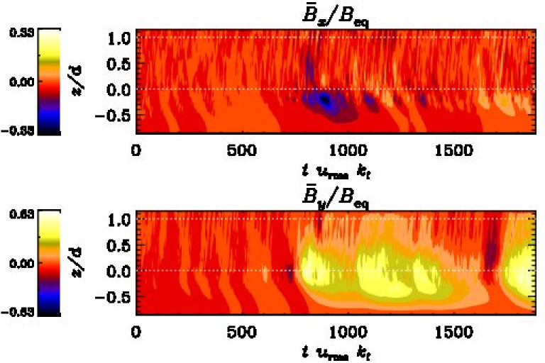
We confirm the results of Tobias et al. (Tobiasea2008 (2008)) in the case where the horizontal boundaries are periodic and find that the rms value of the large-scale (horizontally averaged) field amounts to only a few per cent of the total field. We believe that this is due to the inefficiency of the magnetic helicity flux through the vertical boundaries. In this case the isocontours of shear are horizontal and thus the shear-mediated flux, which we conjecture to be efficient, cannot leave the system. To test this hypothesis, we have made additional runs where the $x$-direction is no longer periodic but instead a stress-free boundary condition for velocity and a normal-field condition for the magnetic field according to

$$U_{x}=U_{y,x}=U_{z,x}=B_{y}=B_{z}=0$$ (18)

is used. In this case the shear-mediated magnetic helicity flux can escape through the $x$-boundaries and significant (up to 50 per cent of the total) large-scale magnetic fields are indeed produced, see Fig. 17. This result lends credence to the hypothesis that the shear-induced flux is an important ingredient in allowing large-scale dynamos to saturate to full strength on a dynamical timescale.

In order to illuminate the circumstances around the time when the mean toroidal field becomes suddenly quite weak ($tu_{\rm rms}k_{\rm f}\approx 1600$), we show in Fig. 18 the mean fields in the cross-stream and streamwise directions. Note that there is no field reversal associated with the sudden drop of toroidal magnetic field, as one might have expected from simulations of dynamo action that is driven purely by magnetic buoyancy, as in the work of Cline et al. (Clineea2003 (2003)).

3.8 Surface appearance of large scale field

In order to make contact with observations, one must eventually compute the field as it would be observable at the surface of the domain. This process can be rather complicated and would involve radiation transfer of polarized light. Here we consider instead just the vertical components of the magnetic field at the top of the convectively unstable layer at $z=z_{3}$; see Fig. 19.

Figure 19: Vertical magnetic field component at the top of the convectively unstable layer at $z=z_{3}$ for Run D2–wide toward the end of the run. The plot is oriented such that the mean shear flow points to the left in the lower part of the plot ($x/d=4$) and to the right in the upper part of the plot ($x/d=-4$). See also http://www.helsinki.fi/$\sim$kapyla/movies.html

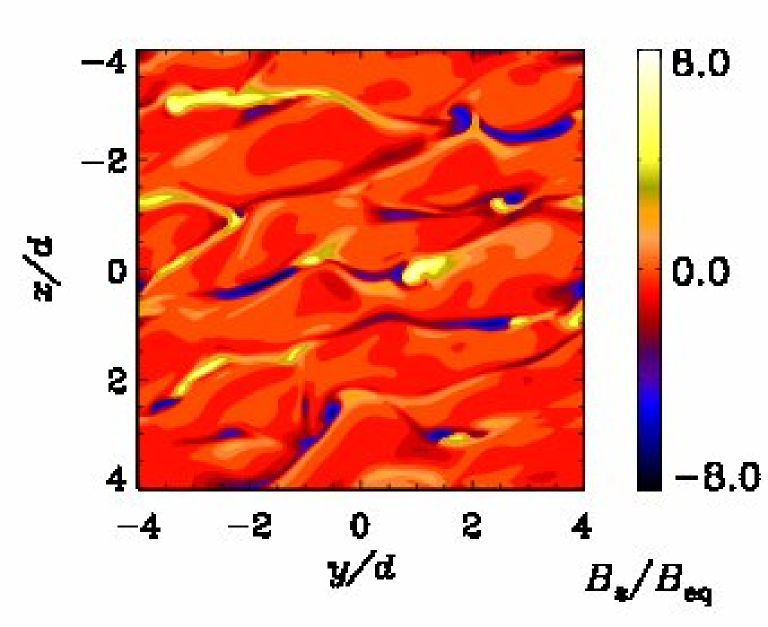
Two things are immediately evident: firstly, the magnetic structures tend to be inclined by up to 30 degrees relative to the $y$-direction and, secondly, there are bipolar regions with a systematic magnetic field orientation such that a negative polarity follows a positive one, which is in agreement with an overall positive mean toroidal field. Comparing with a similar plot of Brandenburg (Brandenburg2005 (2005)), the bipolar regions are here much more compact. Also, the inclination is here such that it would correspond to the southern hemisphere, because $\mbox{d}\overline{U}_{y}/\mbox{d}x$ is here negative.

4 Conclusions

The present simulations provide a clear demonstration that convection can produce large-scale magnetic fields of equipartition strengths in an open Cartesian domain with shear crossing the surface. Our results also demonstrate that this is not possible within a comparable time span using a closed domain with perfectly conducting boundaries. The sensitivity on boundary conditions has also been noted in earlier work with forced turbulence and shear (Brandenburg Brandenburg2005 (2005)). This can be interpreted as being due to magnetic helicity fluxes allowing the system to dispose of excess small-scale magnetic helicity along contours of constant shear (Vishniac & Cho VishCho2001 (2001); Brandenburg & Subramanian 2005b ; Subramanian & Brandenburg SB06 (2006)). In our case this is the vertical direction, but in Tobias et al. (Tobiasea2008 (2008)), it is the horizontal direction. Thus, in our case shear-driven magnetic helicity flux can escape the domain whereas in theirs it cannot due to the periodicity in the horizontal directions. This could explain why no large-scale dynamo develops in their case. Their model is otherwise similar to ours (same values of ${\rm Co}$ and ${\rm Pm}$, whilst ${\rm Rm}$ is about two times smaller, and ${\rm Sh}$ is twice as large.) Control simulations show that replacing their periodic boundary condition in the $x$ direction by a normal-field boundary condition allows strong large-scale fields also in their setup (Fig. 17).

The precise nature of the dynamo found here cannot be pinned down rigorously unless one is able to identify unambiguously the mechanisms that are actively at work. In addition to the $\alpha$-effect, there are other possible alternatives, in particular the incoherent alpha-shear dynamo (Vishniac & Brandenburg VishBran1997 (1997); Proctor Proctor2007 (2007)), which could produce a large-scale magnetic field even without stratification and hence no regular $\alpha$-effect. This interpretation has been favoured in some recent work where the shear–current effect was found not to be excited (Brandenburg et al. Brandea2008 (2008)). However, this matter is still under debate and there are arguments in favour of a shear–current effect (e.g. Kleeorin & Rogachevskii KleRoga2008 (2008)).

In order to disentangle the relative roles of different mechanisms in the present work it will be important to establish a closer connection with mean-field theory by determining the components of the $\alpha$ and turbulent magnetic diffusivity tensors for different boundary conditions and as a function of ${\rm Rm}$. Only when the results are shown to be converged with ${\rm Rm}$ may we expect them to be relevant for the Sun and perhaps other astrophysical bodies.

We emphasize that large-scale dynamo action is normally only seen in the nonlinear stage, whilst the linear stage is dominated by small-scale magnetic fields. It is therefore important to consider mean-field transport coefficients that are affected by the magnetic field. It is in principle even possible that the relevant dynamo mechanism is an intrinsically nonlinear one, as it is in the case of accretion disc turbulence where the turbulence is the result of the dynamo itself (Brandenburg et al. Brandea1995 (1995)). The present results do not give any indications in this direction, because there seems to be a continuous transition from low-${\rm Rm}$ to higher-${\rm Rm}$ large scale dynamo action. For example at ${\rm Rm}=11$, small-scale dynamo action in the usual sense is not expected, and nevertheless, the final saturation strength of the large-scale field is similar to the case of higher-${\rm Rm}$ dynamos.

Another important aspect to consider in future work is the degree of scale separation. As the Reynolds number increases, the turbulence becomes more vigorous and the convection plumes will no longer penetrate the entire depth of the unstable layer. Therefore, we expect the wavenumber of the energy-carrying eddies to increase, i.e. $k_{\rm f}>2\pi/d$. This means that the degree of scale separation, i.e. the ratio $k_{\rm f}/k_{1}$, will also increase. However, as discussed at the end of Sect. 3.4, more scale separation is only expected to enhance large-scale dynamo action.