Fluctuations in granular gases

Abstract

A driven granular material, e.g. a vibrated box full of sand, is a stationary system which may be very far from equilibrium. The standard equilibrium statistical mechanics is therefore inadequate to describe fluctuations in such a system. Here we present numerical and analytical results concerning energy and injected power fluctuations. In the first part we explain how the study of the probability density function (pdf) of the fluctuations of total energy is related to the characterization of velocity correlations. Two different regimes are addressed: the gas driven at the boundaries and the homogeneously driven gas. In a granular gas, due to non-Gaussianity of the velocity pdf or lack of homogeneity in hydrodynamics profiles, even in the absence of velocity correlations, the fluctuations of total energy are non-trivial and may lead to erroneous conclusions about the role of correlations. In the second part of the chapter we take into consideration the fluctuations of injected power in driven granular gas models. Recently, real and numerical experiments have been interpreted as evidence that the fluctuations of power injection seem to satisfy the Gallavotti-Cohen Fluctuation Relation. We will discuss an alternative interpretation of such results which invalidates the Gallavotti-Cohen symmetry. Moreover, starting from the Liouville equation and using techniques from large deviation theory, the general validity of a Fluctuation Relation for power injection in driven granular gases is questioned. Finally a functional is defined using the Lebowitz-Spohn approach for Markov processes applied to the linear inelastic Boltzmann equation relevant to describe the motion of a tracer particle. Such a functional results to be different from injected power and to satisfy a Fluctuation Relation.

1 Introduction

In equilibrium thermodynamics one characterizes the stable phases of a system using a limited set of macroscopic state variables, therefore bypassing much of the microscopic details of the systems under study. It is only very recently that the same strategy has been applied to systems in Non-Equilibrium Steady-States (NESS). And the need for such an approach is all the more pregnant for the study of NESS that no general formalism parallel to the standard equilibrium Gibbs-Boltzmann ensemble theory exists. This field started with experiments carried out on turbulent flows or convection cells, and much more recently on granular systems. Global observables, namely spatially integrated over the whole system, and their distribution, may indeed coarse-grain the irrelevant microscopic details specific to the system at hand, while allowing for comparisons between different systems. They are expected to be more robust and more exportable tools for analysis than local probes, like e.g. structure factors. This has led to the observation of intriguing similarities between turbulent flows and granular systems BHP (98); BdSMRM (05); Ber (05). However, one must take into account the key ingredient making a NESS way different from its equilibrium counterpart: steady flows of energy, matter, or else, run across the system. The existence of currents characterizes a NESS, and makes it different from an equilibrium state in that detailed balance (time reversibility) no longer holds. Given that the time direction plays a central rôle, one is led to the idea that time integration may also be useful in smoothening out various details of the microscopic dynamics. This has motivated several authors to consider the distribution of time integrated and spatially averaged quantities characterizing the NESS as such, like that of the injected power in a turbulent flow or in a granular gas.

We briefly turn to a reminder of phenomenological thermodynamics of nonequilibrium systems, as presented in dGM (69). There, for systems only slightly away from equilibrium, the concept of entropy can be extended in a consistent fashion, and its time evolution goes according to

$$\frac{dS}{dt}=\int_{V}\sigma_{\text{irr}}-\int_{V}\nabla\cdot{\bf J}_{S}.$$ (1)

The intrinsic entropy production rate $\sigma_{\text{irr}}$ is positive definite, and cancels under the condition that the system reaches equilibrium. The other piece in the rhs of (1), which features an entropy current ${\bf J}_{S}$, conveys the existence of external sources, often located at the system’s boundaries, driving the system out of equilibrium. The entropy current is not but a linear combination of the various currents flowing through the system, with the conjugate affinities (like a temperature or a chemical potential gradient) as the proportionality factors. The entropy current – when it can univoquely be defined – therefore stands as a relevant measure of how far the system is from equilibrium. For that reason, various studies, starting from the pioneering work of Evans, Cohen and Morriss ECM (93), in a study of a thermostatted fluid under shear, have been focused on the appropriately generalized expression of the latter entropy current. In Evans, Cohen and Morriss’ case it is simply proportional to the power provided by the thermostat to compensate for viscous dissipation. They went on to determine the distribution function of $Q_{S}(t)$, the time integrated entropy flow (or equivalently the energy provided by the thermostat), denoted by $P(Q_{S},t)$. In doing so they empirically noticed a remarkable property of the pdf of $Q_{S}$, namely

$$\lim_{t\to\infty}\frac{1}{t}\log\frac{P(Q_{S},t)}{P(-Q_{S},t)}=q_{S},$$ (2)

where $q_{S}=Q_{S}/t$, which is a time-intensive quantity, is the time average of $J_{S}$ over $[0,t]$. This symmetry property of the pdf of $Q_{S}$ was soon to be formalized into a theorem for thermostatted systems by Gallavotti and Cohen GC (95), and has since triggered a flurry of studies. The mathematical object defined by $\pi(q_{S})=\lim_{t\to\infty}\frac{\log P(q_{S}\;t,t)}{t}$ is seen to be extending the concept of intensive free energy to a nonequilibrium setting, and will occupy much of our numerical and analytical efforts.

In the realm of nonequilibrium systems, granular gases play a central rôle as systems exhibiting a strongly irreversible microscopic dynamics due to inelastic collisions, and for these no viable definition of entropy, let alone entropy flow, is available. This has led various authors AFMP (01); FM (04) to conjecture that, by analogy to thermostatted systems, the power injected into the system to maintain it in a steady-state, could satisfy a symmetry property like the one uncovered by ECM (93), and its ensuing consequences in terms of generalized fluctuation–dissipation theorems. Fortunately, a well-controlled kinetic theory-based statistical mechanics exists for dilute gaseous systems, and we shall build upon it to investigate the questions raised above.

The outline of the present review is as follows. We begin in Sec. 2 with a brief introduction to granular gases and the basics of their statistical mechanics. In Sec. 3 we analyze the distribution of the total kinetic energy of the gas, as a first choice for a global observable. In Sec. 4 and 5 we address numerically, analytically and also experimentally, the issue of interpreting the power injected into a gas in terms of entropy flow, the negative outcome of which leads us to Sec. 6. There we construct a one particle observable exhibiting the properties expected from an entropy flow, and quite notably its distribution function displays the symmetry property (2).

2 A brief introduction to granular gases

A granular gas is an assembly of macroscopic particles kept in a gaseous steady state by a constant excitation BTE (05)(the typical example can be illustrated thinking of many beads in a strongly vibrated box). The simplest way to characterize such systems is to consider $N$ identical smooth hard spheres, losing a part of their kinetic energy after each collision. The total momentum is conserved in collisions, and only the normal component of the velocity is affected. Thus, the collision law for a couple of particles $(1,2)$ reads:

$$\begin{cases}{\bf v}_{1}^{*}={\bf v}_{1}-{1\over 2}(1+\alpha)({\bf v}_{12}\cdot{\hat{\boldsymbol{\sigma}}}){\hat{\boldsymbol{\sigma}}}\\ {\bf v}_{2}^{*}={\bf v}_{2}+{1\over 2}(1+\alpha)({\bf v}_{12}\cdot{\hat{\boldsymbol{\sigma}}}){\hat{\boldsymbol{\sigma}}}\,\,,\\ \end{cases}$$ (3)

where $\hat{\boldsymbol{\sigma}}$ is a unitary vector along the center of the colliding particles at contact. Here $\alpha$ is a constant, called the coefficient of normal restitution ($0\leq\alpha\leq 1$, and when $\alpha=1$ collisions are purely elastic). Without some energy injection mechanism the total energy of the gas will decrease in time, until all the particles are at rest (cooling state). However, when some energy input is provided, the system can reach a nonequilibrium stationary state. Energy injection may be supplied in several ways, which can be divided in two main categories: injection from the boundaries and homogeneous driving. In the former category energy is supplied by a boundary condition, the system hence develops spatial gradients and it is not homogeneous. The latter category refers to systems where energy injection is achieved by a homogeneous and isotropic force acting on each particle.

A granular gas is a gas of inelastic particles. Models for granular gases divide into two main classes: driven models and cooling models. The first class includes inelastic gases with an energy external source that asymptotically guarantees a stationary state. The second class is that of “free” inelastic gases, whose dissipative dynamics eventually leads to a state of complete rest. Here we recall the definition of the homogeneous driven gas of inelastic hard disks, which is the most used in this chapter. Other models can be easily obtained from this main model changing some ingredients: the homogeneous cooling gas of inelastic hard disks is obtained eliminating the external stochastic forcing, while the boundary driven gas of inelastic hard disks is obtained replacing the stochastic forcing with a vibrating container.

2.1 Boundary driven gases

In this section we will give a short introduction to the methods used to describe the behavior of a granular gas in which energy is injected by a boundary condition (typically a vibrating wall). This kind of system has been widely studied in the literature GZBN (97); MB (97); ML (98); Kum (98); BRMM (00); BT (02), and one of its main characteristics is that the density and the temperature are not homogeneous over the system: there is a heat flux, which does not verify Fourier law. This feature is well described by kinetic theory and in good agreement with the hydrodynamic approximation, which allows an analytical calculation of the density and temperature profiles. In the dilute limit, such a system is well described by the Boltzmann equation:

$$\partial_{t}f({\bf r},{\bf v}_{1},t)+{\bf v}_{1}\cdot{\boldsymbol{\nabla}}f({\bf r},{\bf v}_{1},t)=J[f|f]\,\,.$$ (4)

Here $J[f|f]$ is the collision integral, which takes into account the inelasticity of the particles:

$$J[f|f]=\sigma^{d-1}\int\textrm{d}{\bf v}_{2}\int^{\prime}\textrm{d}\hat{\boldsymbol{\sigma}}({\bf v}_{12}\cdot\hat{\boldsymbol{\sigma}})\left(\frac{f({\bf v}_{1}^{**},t)f({\bf v}_{2}^{**},t)}{\alpha^{2}}-f({\bf v}_{1},t)f({\bf v}_{2},t)\right),$$ (5)

where the notation ${\bf v}_{12}$ denotes the relative velocity between particles 1 and 2, the two stars superscript (i.e. ${\bf v}^{**}$) denote the precollisional velocity of a particle having velocity ${\bf v}$, and the primed integral is a short-hand notation meaning that the integration is performed on all angles satisfying $\mathbf{v}_{12}\cdot\hat{\boldsymbol{\sigma}}>0$. The hydrodynamic fields are defined as the velocity moments:

$$n({\bf r},t)=\int\textrm{d}{\bf v}f({\bf r},{\bf v},t)\,,$$ (6)

$$n({\bf r},t){\bf u}({\bf r},t)=\int\textrm{d}{\bf v}\,{\bf v}f({\bf r},{\bf v},t)\,,$$ (7)

$${d\over 2}n({\bf r},t)T({\bf r},t)=\int\textrm{d}{\bf v}{m\over 2}({\bf v}-{\bf u})^{2}f({\bf r},{\bf v},t)\,,$$ (8)

and the hydrodynamic balance equations for those quantities are derived taking the velocity moments in the equation (4). Their expression is:

$$\partial_{t}n+\nabla\cdot\left(n\mathbf{u}\right)=0,$$ (9)

$$\left(\partial_{t}+\mathbf{u}\cdot\nabla\right)u_{i}+(mn)^{-1}{\nabla}_{j}P_{ij}=0,$$ (10)

$$\left(\partial_{t}+\mathbf{u}\cdot\nabla+\zeta\right)T+\frac{2}{3n}\left(P_{ij}{\nabla}_{j}u_{i}+\nabla\cdot\mathbf{q}\right)=0,$$ (11)

where the pressure tensor $P_{ij}$, heat flux $\mathbf{q}$, and the cooling rate $\zeta$ are defined by:

$$P_{ij}(\mathbf{r},t)=\int d\mathbf{v}\,m(v_{i}-u_{i})(v_{j}-u_{j})f(\mathbf{r},\mathbf{v},t)\,\,,$$ (12)

$$\mathbf{q}(\mathbf{r},t)=\int d\mathbf{v}\frac{m}{2}(\mathbf{v}-\mathbf{u})^{2}(\mathbf{v}-\mathbf{u})f(\mathbf{r},\mathbf{v},t)\,\,,$$ (13)

$$\zeta(\mathbf{r},t)=\frac{(1-\alpha^{2})m\pi^{\frac{d-1}{2}}\sigma^{d-1}}{4d\Gamma\left(\frac{d+3}{2}\right)n(\mathbf{r},t)T(\mathbf{r},t)}\int\,\textrm{d}\mathbf{v}_{1}\,\int\,\textrm{d}\mathbf{v}_{2}\,|v_{12}|^{3}\ f(\mathbf{r},\mathbf{v}_{1},t)f(\mathbf{r},\mathbf{v}_{2},t).$$ (14)

Explicit analytical expressions for the above quantities have been obtained in the limit of small spatial gradients by Brey et al. BDKS (98); BC (01). Moreover for systems in the steady state without a macroscopic velocity flow the hydrodynamic equations simplify, and therefore the temperature and density profiles can be explicitly computed.

2.2 Randomly driven gases

We consider here a granular gas kept in a stationary state by an external homogeneous thermostat, the so called “Stochastic thermostat”, which couples each particle to a white noise. Energy injection is hence achieved by means of random forces acting independently on each particle, and drives the gas into a non-equilibrium steady state. The equation of motion governing the dynamics of each particle is therefore:

$$m{\textrm{d}{\bf v}_{i}\over\textrm{d}t}={\bf F}_{i}^{\text{coll}}+{\bf F}_{i}^{\text{th}},$$ (15)

where ${\bf F}_{i}^{\text{coll}}$ is the force due to collisions and ${\bf F}_{i}^{\text{th}}$ is a Gaussian white noise (i.e. $\langle F_{i\gamma}^{\text{th}}(t)F_{j\delta}^{\text{th}}(t^{\prime})\rangle=2\Gamma\delta_{ij}\delta_{\gamma\delta}\delta(t-t^{\prime})$, where the subscripts $i$ and $j$ are used to refer to the particles, while $\gamma$ and $\delta$ denote the Euclidean components of the random force). This model is one of the most studied in granular gas theory and reproduces many qualitative features of real driven inelastic gases WM (96); PO (98); PLM⁺ (98); vNETP (99); HBB (00); MSS (01); PTvNE (02); vNE (98). After a few collisions per particle the system attains a non-equilibrium stationary state. This state seems homogeneous. From the equations of motion it is possible to derive the homogeneous Boltzmann equation governing the evolution of the one-particle velocity distribution function vNE (98):

$$\partial_{t}f({\bf v}_{1},t)=J[f,f]+\Gamma\Delta_{{\bf v}_{1}}f({\bf v}_{1})\,\,,$$ (16)

where the Laplace operator $\Delta_{{\bf v}}\equiv(\partial/\partial_{{\bf v}})^{2}$ is a diffusion term in velocity space characterizing the effect of the random force, while $J[f,f]$ is the collision integral, which takes into account the inelasticity of the collisions (cf. eq. (5)). The granular temperature of the system is defined as usual as the mean kinetic energy per degree of freedom, $T_{g}=\langle v^{2}\rangle/d$. The stationary solution of equation (16) has extensively been investigated in the last years. Even if an exact solution is still missing, a general method is to look for solutions in the form of a Gaussian distribution multiplied by a series of Sonine polynomials CC (60):

$$f_{st}({\bf v})=e^{-{v^{2}\over 2T_{g}}}\left(1+\sum_{p=1}^{\infty}a_{p}S_{p}\left({v^{2}\over 2T_{g}}\right)\right)\,\,.$$ (17)

The expression of the first three Sonine polynomials is:

$$S_{0}(x)=1$$

$$S_{1}(x)=-x+{1\over 2}d$$ (18)

$$S_{2}(x)={1\over 2}x^{2}-{1\over 2}(d+2)x+{1\over 8}d(d+2)\,\,.$$

Moreover the coefficients $a_{p}$ are found to be proportional to the averaged polynomial of order $p$:

$$a_{p}=A_{p}\left\langle S_{p}\left({v^{2}\over 2T_{g}}\right)\right\rangle\,\,,$$ (19)

where $A_{p}$ is a constant and the angular brackets denote average with weight $f_{st}$. From this observation one directly obtains that the first coefficient $a_{1}$ vanishes by definition of the temperature. A first approximation for the velocity pdf is therefore to truncate the expansion up to the second order ($p=2$). An approximated expression for the coefficient $a_{2}$ has been found as a function of the restitution coefficient $\alpha$ and the dimension $d$ vNE (98); CDPT (03); MS (00). Its expression is:

$$a_{2}(\alpha)={16(1-\alpha)(1-2\alpha^{2})\over 73+56d-24\alpha d-105\alpha+30(1-\alpha)\alpha^{2}}\,\,.$$ (20)

It must be noted that the second Sonine approximation is only valid for not too large velocities, since the tails of the pdf have been shown  vNE (98) to be overpopulated with respect to the Gaussian distribution. It is known vNE (98) that in high energies $\log f(v)\sim-(v/v_{c})^{3/2}$ with a threshold velocity $v_{c}$ that diverges when the dimension $d$ goes to infinity. This means that at high dimensions the distribution is almost a Gaussian, since both the tails and the $a_{2}$ contributions tend to vanish. All the above results have been confirmed by numerical simulations, in particular through Molecular Dynamics (MD) and Direct simulation Monte Carlo (DSMC) Bir (94) methods. Those two numerical methods, although very different, show a surprisingly good agreement. This points out to correctness of the molecular chaos assumption and thus to the relevance of the DSMC method, which is particularly well adapted to simulate the dynamics of a homogeneous dilute gas.

3 Total energy fluctuations in vibrated and driven granular gases

3.1 The inhomogeneous boundary driven gas

In this section we will study the energy fluctuations of a granular gas in the case where the energy is injected into the system by a vibrating wall. Recently Aumaître et al. AFFM (04) investigated, by means of Molecular Dynamic (MD), the fluctuations of the total energy of the system. In particular they looked at the behavior of the first two moments of the energy pdf when the system size is changed, at constant averaged density. Because of the inhomogeneities, the mean kinetic energy is no more proportional to the number of particles, and thus it is not an extensive quantity, and analogously the mean kinetic temperature is no more intensive. This has led to the definition of an effective (intensive) temperature and an effective number of particles, which makes the energy extensive. In the following we will show how a rough calculation (neglecting correlations and small non-Gaussianity) using the hydrodynamic prediction for the temperature profile VPB⁺06b , can explain the phenomenology observed in AFFM (04). Within this description it is possible to get an expression of the effective temperature and number of particles as a function of the system parameters (i.e. number of particles, restitution coefficient, and temperature of the vibrating wall).

Energy Probability Distribution Function

In this part we will compute the energy pdf for a granular gas between two (infinite) parallel walls. The distance between the two walls is denoted by $H$, oriented along the $x$ axis. Here we assume that one of the walls (in $x=0$) has small and random vibrations, acting as a thermostat that fixes to $T_{0}$ the temperature at $x=0$. Our boundary conditions therefore are:

$$T(\ell=0)=T_{0}\,\,,\,\,\,\,\,\,\,\,\,\,\left.\frac{\partial T}{\partial\ell}\right|_{\ell=\ell_{m}}=\,\,\left.\frac{\partial T}{\partial x}\right|_{x=H}=0\,\,,$$ (21)

where the rescaled length $\ell$ will be defined below. For the particular case of a steady state without macroscopic velocity flow, is it possible to solve those balance equations and get the temperature profile BRMM (00):

$$T(\ell)=T_{0}\left({\cosh{\left(\sqrt{a(\alpha)}(\ell_{m}-\ell)\right)}\over\cosh{\left(\sqrt{a(\alpha)}\ell_{m}\right)}}\right)^{2}\,\,,$$ (22)

where $a(\alpha)$ is a function of the restitution coefficient (its complete expression is given in ref. BdSMRM (04)). The variable $\ell$ is proportional to the integrated density of the system on the $x$ axis. Its definition is given by the following relation involving the local mean-free-path $\lambda(x)$:

$$\textrm{d}\ell={\textrm{d}x\over\lambda(x)}\,\,,\lambda(x)=\left[{\sqrt{2}\pi^{d-1\over 2}\over\Gamma[(d+1)/2]}\sigma^{d-1}n(x)\right]^{-1}\,\,.$$ (23)

In the following we will suppose the velocity distribution to be a Maxwellian (a small non-Gaussian behavior exists, but it is not relevant for this calculation) with a local temperature (variance) given by (22):

$$f({\bf v},\ell)={e^{-{v^{2}\over 2T(\ell)}}\over{(2\pi T(\ell))^{d/2}}}\,\,.$$ (24)

The distribution for the energy of one particle ($e=v^{2}/2$) is hence:

$$p(e,T(\ell))=f_{{1\over T(\ell)},{d\over 2}}(e)\,\,\,,$$ (25)

where $f_{\alpha,\nu}(x)$ is the gamma distribution Fel (71):

$$f_{\alpha,\nu}(x)={\alpha^{\nu}\over\Gamma(\nu)}x^{\nu-1}e^{-\alpha x}\,.$$ (26)

Our interest goes to the macroscopic fluctuations integrated over all the system. Thus, the macroscopic variable of interest is the granular temperature $T_{g}$, defined here as the average of the local temperature over the $x$ profile:

$$T_{g}={1\over N}\int_{V}n({\bf r})T({\bf r})\,\,\textrm{d}{\bf r}={1\over\ell_{m}}\int_{0}^{\ell_{m}}T(\ell)\,\,\textrm{d}\ell\,\,.$$ (27)

with

$$\ell_{m}=N_{x}\frac{\sqrt{2}\pi^{\frac{d-1}{2}}\sigma^{d-1}}{\Gamma[(d+1)/2]},\;\;\;N_{x}=\frac{N}{V_{d-1}},$$ (28)

where $V_{d-1}$ is the area of the surface of dimension $d-1$ orthogonal to the $x$-direction, i.e. $H\times V_{d-1}=V$. When $d=2$ one has $V_{d-1}\equiv L$ where $L$ is the width of the system. $N_{x}$ is the number of particles per unit of section perpendicular to the $x$ axis. To get an expression of the energy pdf over the whole system, it is useful to divide the box in $\ell_{m}/\Delta\ell$ boxes of equal height (in the $\ell$ scale) $\Delta\ell$. It is helpful to use the length scale $\ell$ because the number of particles $N_{\ell}$ in each box of size $L\times\Delta\ell$ is a constant. Moreover, in each box $i$ we will suppose the temperature a constant $T_{i}\equiv T(i\,\,\Delta\ell)$, defined expanding the granular temperature in a Riemann sum:

$$T_{g}=\lim_{\Delta\ell\to 0}\sum_{i=0}^{\ell_{m}/\Delta\ell}T_{i}\,\,\Delta\ell$$ (29)

The calculation of the pdf of the box energy $\epsilon_{i}$, i.e. a sum of the energies of the $N_{\ell}$ particles in a box $i$, is hence straightforward when the velocities of the particles are supposed to be uncorrelated:

$$q_{i}(y)\equiv\textrm{prob}(\epsilon_{i}=y)=f_{{1\over T_{i}},{dN_{\ell}\over 2}}(y)\,\,\,,$$ (30)

The characteristic function of $q_{i}(y)$ is

$$\tilde{q}_{i}(k)=\frac{1}{(1-ikT_{i})^{\frac{dN_{\ell}}{2}}}$$ (31)

Thus, the characteristic function for the kinetic energy of the whole system $E=\sum\epsilon_{i}$ can be obtained as the product of the characteristic functions ${\tilde{q}}_{i}(k)$:

$${\widetilde{P}}(k)=\prod_{j=0}^{\ell_{m}/\Delta\ell}{\tilde{q}}_{j}(k)=\prod_{j=0}^{\ell_{m}/\Delta\ell}{1\over(1-{{\textrm{i}}}kT_{j})^{dN_{\ell}\over 2}}\,\,\,.$$ (32)

Since the number of particle per box $N_{\ell}$ is a known fraction of the total number of particles ($N_{\ell}=N\Delta\ell/\ell_{m}$), one can rewrite the expression (32) as a Riemann sum. In the limit $\Delta\ell\to 0$ this yields the total kinetic energy characteristic function:

$${\widetilde{P}}(k)=\exp\left(\,-{dN\over 2\ell_{m}}\int_{0}^{\ell_{m}}\log\left(1-{{\textrm{i}}}kT(\ell)\right)\,\,\textrm{d}\ell\right)\,\,.$$ (33)

Note that this result is valid for any temperature profile $T(\ell)$ and hence it can be applied also to other situations with different boundary conditions or different hydrodynamic equations.

Comparison with simulations

Aumaître et al. AFMP (01); AFFM (04) showed by Molecular dynamic simulations, that the pdf of the total energy is well fitted by a $\chi^{2}$ law $\Pi(E)=f_{{1\over T_{E}},{N_{f}\over 2}}(E)$ with a number of degrees of freedom $N_{f}$ different from $dN$, and a temperature $T_{E}$ different from the granular temperature $T_{g}$. The two parameters $N_{f}$ and $T_{E}$ are functions of the first two cumulants of the pdf:

$$N_{f}=2\,{\langle E\rangle_{c}^{2}\over{\langle E^{2}\rangle_{c}}}\,,\;\;\;\;\;\;\;\;\;\;\;\;\;\;\;\;\;\;\;\;T_{E}={\langle E^{2}\rangle_{c}\over\langle E\rangle_{c}}\,\,.$$ (34)

The notation $\langle X\rangle_{c}$ denotes the cumulant of the variable $X$. Here we want to compare result (33) with these numerical results. Since we are not able to analytically calculate the inverse Fourier Transform of (33) using (22) as a temperature profile, we used a numerical computation to obtain it in an approximate form. Moreover, an expression of the cumulants of the total kinetic energy can be obtained from the characteristic function (33):

$$\langle E^{p}\rangle_{c}={dN\over 2\ell_{m}}\int_{0}^{\ell_{m}}T^{p}(\ell)\textrm{d}\ell\,\,\,.$$ (35)

In figure 1 the Inverse Fourier Transform of (33) is compared with the function $\Pi(E)$ previously defined. The similarity of the two functions is remarkable. Another important feature that can be checked with this results is the dependence of the above defined two macroscopic quantities ($N_{f}$ and $T_{E}$) with system size. It is straightforward to see, from (27) and (35), that the granular temperature and the total kinetic energy are respectively an intensive and an extensive variable if $\ell_{m}$ is independent from the system size. This is effectively the case if both the density $\rho=N/V$ and the total height $H$ are kept constant. Moreover, for large enough $\ell_{m}$, the integral in equation (35) becomes size independent:

$$\int_{0}^{\ell_{m}}T^{p}(\ell)\textrm{d}\ell\sim{T_{0}^{p}\over 2p\sqrt{a(\alpha)}}\,\,.$$ (36)

Thus, the effective temperature $T_{E}$ defined above becomes a constant proportional to the temperature of the wall, while the parameter $N_{f}$ still depends on the system size:

$$N_{f}\sim{1\over\sqrt{a(\alpha)}}\,{dN\over\ell_{m}}\,,\;\;\;\;\;\;\;\;\;\;\;\;\;\;\;\;\;\;\;\;T_{E}\sim{T_{0}\over 2}.$$ (37)

Numerical simulations show that $T_{E}$ effectively remains a constant for large systems, and under several procedures of box size increase. The behavior of $N_{f}$ is determined by the maximum of the integrated density $\ell_{m}$. For a square cell at constant density one finds $\ell_{m}\propto\sqrt{N}$ , so that $N_{f}\propto\sqrt{N}$, which is not far from $N^{0.4}$ observed in AFFM (04). Moreover, if only the height $H$ of the cell is increased, $\ell_{m}$ is proportional to $N$, and $N_{f}$ becomes constant. All those features are in agreement with the numerical observations in AFFM (04). The above results clearly show that a rough calculation, which takes into account only the inhomogeneities of the system, is able to quantitatively describe the behavior of the fluctuations of the total kinetic energy of a vibrated granular gas. In some cases the energy pdf can be approximated with a gamma distribution, which is the standard distribution for the energy pdf in the canonical equilibrium. Nevertheless there are strong deviations from the equilibrium theory of fluctuations, since the two parameters of the gamma distribution (i.e. the temperature and the number of degrees of freedom) are not the granular temperature neither the number of degrees of freedom. Another important remark is that correlations, and in particular contributions from the two points distribution function, do not play a primary role to explain those deviations from the equilibrium theory of fluctuations. In order to characterize corrections arising from the two particles velocity pdf, one should measure energy fluctuations at a given height $x$ from the vibrating wall. As already noted in AFFM (04) this task is very hard, since the available statistic become very poor. Nevertheless an effective way to quantify those fluctuations is to look at homogeneous systems, where contributions coming from the inhomogeneities vanish. With this objective in mind, we will be interested in the following in granular gases heated by an homogeneous and isotropic driving.

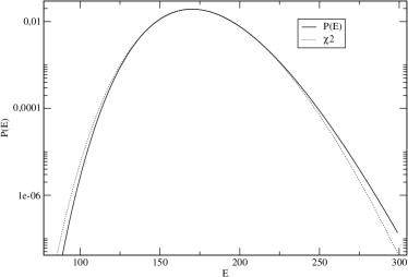
Figure 1: Energy pdf (solid line) and a gamma distribution with same mean and same variance (dotted line) for a restitution coefficient $\alpha=0.9$ , $N=100$ particles in two dimensions in a box of density $\rho=0.04$, height $H=50$, and with a wall temperature $T_{0}=5$.

3.2 The homogeneously driven case

In this section we will present some numerical results concerning the energy fluctuations in a dilute gas driven by the stochastic thermostat presented in section 2.2 VPB⁺06b . When the system reaches a stationary state, the dissipated energy is compensated by the energy injected by the thermostat, and the temperature fluctuates around its mean value. Here we are interested in the fluctuations of the total energy measured by the quantity

$$\sigma_{E}^{2}=N{\langle E^{2}(t)\rangle-\langle E(t)\rangle^{2}\over\langle E(t)\rangle^{2}}\,\,.$$ (38)

Note that $\sigma_{E}^{2}\equiv 2N/N_{f}$. Brey et al. have computed, by means of kinetic equations, an analytical expression for $\sigma_{E}^{2}$ in the homogeneous cooling state, which is equivalent to the so-called Gaussian deterministic thermostat. One of the main differences of this stochastic thermostat with a deterministic one, is found in the elastic limit. On the one hand, for the cooling state, when the restitution coefficient tends to 1, the conservation of energy imposes that the energy pdf is a Delta function, and the quantity $\sigma_{E}$ goes to $0$. On the other hand, with the stochastic thermostat, if the elastic limit is taken keeping the temperature constant, the strength of the white noise will tend to zero, but it will still play a role in the velocity correlation function.

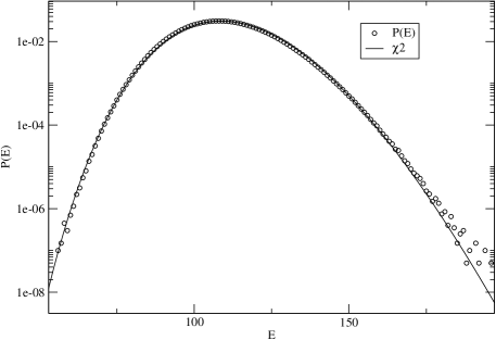
Figure 4: Energy pdf (dots) from DSMC simulations with a restitution coefficient $\alpha=0.5$ and $N=100$ particles for a system driven with the stochastic thermostat. The solid line shows a gamma distribution with same mean and same variance.

We performed DSMC simulations to measure the energy pdf of such a system. A plot of this pdf is shown in figure 4, and it is close to a $\chi^{2}$-distribution with same mean and same variance. Nevertheless the number of degrees of freedom of this $\chi^{2}$-distribution is lower than the true number of degrees of freedom (i.e. $(N-1)\times d$). This effect may arise from two separated causes: the non-gaussianity of the velocity pdf, and the presence of correlations between the velocities. This feature also suggests that a calculation of the energy pdf with the hypothesis of uncorrelated velocities (but non-Gaussian) could explain at least a part of this non-trivial effect. In order to quantify these contributions we will consider that the velocity pdf is well described by a Gaussian multiplied by the second Sonine polynomial:

$$f(v)=\frac{e^{-\frac{v^{2}}{2T}}}{(2\pi T)^{d/2}}\left(1+a_{2}S_{2}\left(\frac{v^{2}}{2T}\right)\right)\,\,,$$ (39)

where $a_{2}$ is given by expression (20).

The calculation of the pdf of the sum of the square of $N$ variables distributed following (39) is straightforward. The characteristic function of the energy pdf is:

$${\widetilde{P}}_{N}(k)={1\over(1-{{\textrm{i}}}kT)^{Nd\over 2}}\ \left(1+{d(d+2)\over 8}a_{2}\left({1\over(1-{{\textrm{i}}}kT)^{2}}-{2\over(1-{{\textrm{i}}}kT)}+1\right)\right)^{N}$$ (40)

where $N$ is the number of particles of the system. This yields:

$$\langle E\rangle={d\over 2}NT\,\,,\;\;\;\;\;\;\;\;\;\;\;\;\;\;\;\;\;\;\;\;\langle E^{2}\rangle-\langle E\rangle^{2}={d\over 2}NT^{2}\left(1+{d+2\over 2}a_{2}\right)\,\,.$$ (41)

It is now possible to have an explicit expression for the energy fluctuations:

$$\sigma^{2}_{E_{(uncorr.)}}={2\over d}\left(1+{d+2\over 2}a_{2}\right)\,\,.$$ (42)

In figure 5 this result is compared with the result of DSMC simulations, performed for several values of the restitution coefficient $\alpha$ and for two different values for the number of particles $N$. The disagreement between the uncorrelated calculation and the simulations is a clear sign of the correlations induced by the inelasticity of the system. One can note that the fluctuations increase when the restitution coefficient decreases. One can also see that there is a value of the restitution coefficient $\alpha$ around $1/\sqrt{2}$, that is when the approximate expression of $a_{2}$ vanishes, for which $\sigma_{E}^{2}$ is exactly $1\equiv 2/d$, as for a gas in the canonical equilibrium (velocities are then uncorrelated).

We now turn to the dependence of $\sigma^{2}_{E}$ on the strength of the white noise $\Gamma$. It is useful, for this purpose, to introduce a rescaled, dimensionless energy

$${\widetilde{E}}={E-\langle E\rangle\over\sqrt{\langle E^{2}\rangle-\langle E\rangle^{2}}}\,\,.$$ (43)

We have plotted in figure 6 this rescaled energy pdf for a system of $N=100$ particles with a restitution coefficient $\alpha=0.5$ and for several values of the strength of the white noise $\Gamma$. One can see how all the pdfs collapse into a unique distribution. The role of the noise’s strength is thus only to set the temperature (or mean kinetic energy) scale. Besides, relative energy fluctuations depend only on $\alpha$ and $N$. Moreover, since $\sigma_{E}^{2}$ does not depend on the number of particles $N$ (for $N$ large enough), the central limit theroem applies, and hence $P({\tilde{E}})$ is a Gaussian in the thermodynamic ($N\to\infty$) limit. Another important unexpected result is that these fluctuations are independent from the strength of the random force. In order to show this feature is useful to introduce a rescaled, dimensionless energy

$${\widetilde{E}}={E-\langle E\rangle\over\sqrt{\langle E^{2}\rangle-\langle E\rangle^{2}}}\,\,.$$ (44)

We have plotted in figure 6 this rescaled energy pdf for a system of $N=100$ particle with a restitution coefficient $\alpha=0.5$ and for several values of the strength of the white noise $\Gamma$. One can see how all the pdfs collapse into a unique universal form. This means in particular that correlations are independent from the strength of the noise, while one typically should expect that increasing the strength of the noise correlations should tend to disappear. In conclusion we have shown that randomly driven granular gases display non trivial fluctuations, because of the correlations induced by the inelasticity. Two different kinds of correlations contribute to this behavior of the fluctuations. First, the non-Gaussianity of the velocity pdf, which simply tells that the Euclidean components of the velocity of each particle are correlated one to each other. Second, a contribution from the two particles velocity pdf, which does not factorize exactly as a product of two one-particle distributions. It must be pointed out, however, that these correlations do not invalidate the Boltzmann equation. As already noted in EC (81); BdSMRM (04); CPM (07), the two points correlation function $g_{2}({\bf v}_{1},{\bf v}_{2})$, which is defined by:

$$g_{2}({\bf v}_{1},{\bf v}_{2})=f^{(2)}({\bf v}_{1},{\bf v}_{2})-f({\bf v}_{1})f({\bf v}_{2})\,\,,$$ (45)

where $f^{(2)}$ is the two points distribution, is of higher order in the density expansion (roughly speaking ${\cal O}\left(g({\bf v}_{1},{\bf v}_{2})\right)\sim{\cal O}\left(f({\bf v}_{1})f({\bf v}_{2})\right)/N$). This is confirmed by the numerical observations, since when the number of particles increases, the energy pdf tends be closer and closer to a Gaussian. Spatial correlations, which can be at work in homogeneously driven granular gases, at higher densities, and which have been negleted here (assuming spatial homogeneity) can also play a relevant role in fluctuations PBV (07).

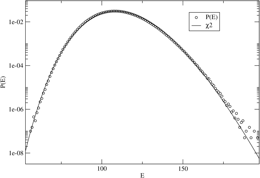
Figure 2: Energy pdf (dots) from DSMC simulations with a restitution coefficient $\alpha=0.5$ and $N=100$ particles for a system driven with the stochastic thermostat. The solid line shows a gamma distribution with same mean and same variance.

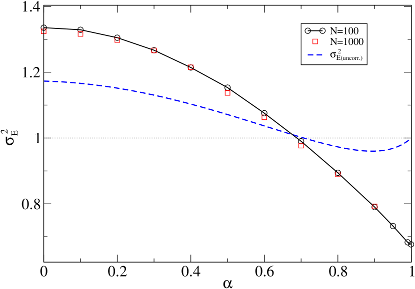
Figure 3: Plot of $\sigma^{2}_{E}$ versus the restitution coefficient $\alpha$ for $N=100$ ($\bigcirc$) and $N=1000$ ($\square$) particles. The result of the calculation assuming uncorrelated velocities (42) is plotted as a dashed line.

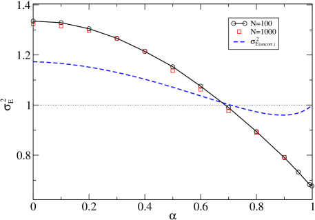
Figure 5: Plot of $\sigma^{2}_{E}$ versus the restitution coefficient $\alpha$ for $N=100$ ($\bigcirc$) and $N=1000$ ($\square$) particles. The result of the calculation assuming uncorrelated velocities (42) is shown by the dashed line.

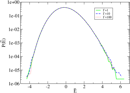
Figure 6: Plot of the pdf of the rescaled energy ${\widetilde{E}}$ for a restitution coefficient $\alpha=0.5$ and for $N=100$ for several values of the strength of the noise $\Gamma$.

4 A large deviation theory for the injected power fluctuations in the homogeneous driven granular gas

From now on we turn our attention to the fluctuations of another global quantity, i.e. the power injected into the system by the external source of energy. In particular in this section our main goal is to obtain a kinetic equation able to describe the behavior of the large deviations function of the time integrated injected power VPB⁺ (05); VPB⁺06a in a randomly driven gas (cf section 2.2). The latter quantity is the total work ${\cal W}$ provided by the thermostat over a time interval $[0,t]$:

$${\cal W}(t)=\int_{0}^{t}\textrm{d}t\sum_{i}{\bf F}^{th}_{i}\cdot{\bf v}_{i}\,.$$ (46)

Our interest goes to the distribution of ${\cal W}(t)$, denoted by $P({\cal W},t)$, and to its associated large deviation function $\pi_{\infty}(w)$ defined for the reduced variable $w={\cal W}/t$ (${\cal W}(t)$ being extensive in time):

$$\pi_{\infty}(w)=\lim_{t\to\infty}\pi_{t}(w)\,\,\,,\pi_{t}(w)=\frac{1}{t}\log P({\cal W}=wt,t)\,.$$ (47)

We introduce $\rho(\Gamma_{N},{\cal W},t)$ the probability that the system is in state $\Gamma_{N}$ at time $t$ with ${\cal W}(t)={\cal W}$. The function we want to calculate is

$$P({\cal W},t)=\int\textrm{d}\Gamma_{N}\rho(\Gamma_{N},{\cal W},t).$$ (48)

We shall focus on the generating function of the phase space density

$$\hat{\rho}(\Gamma_{N},\lambda,t)=\int\textrm{d}{\cal W}\text{e}^{-\lambda{\cal W}}\rho(\Gamma_{N},{\cal W},t)$$ (49)

and on the large deviation function of

$$\hat{P}(\lambda,t)=\int\textrm{d}{\cal W}\text{e}^{-\lambda{\cal W}}P({\cal W},t)=\int\textrm{d}\Gamma_{N}\hat{\rho}(\Gamma_{N},\lambda,t)$$ (50)

which we define as

$$\mu(\lambda)=\lim_{t\to\infty}\frac{1}{t}\log\hat{P}(\lambda,t)\,\,.$$ (51)

Note that $\mu(\lambda)$ is the generating function of the cumulants of ${\cal W}$, namely

$$\lim_{t\to\infty}\frac{\langle{\cal W}^{n}\rangle_{c}}{t}=(-1)^{n}\left.\frac{\textrm{d}^{n}\mu(\lambda)}{\textrm{d}\lambda^{n}}\right|_{\lambda=0}$$ (52)

Moreover $\pi_{\infty}(w)$ can be obtained from $\mu(\lambda)$ by means of a Legendre transform, i.e. $\pi_{\infty}(w)=\mu(\lambda_{*})+\lambda_{*}w$ with $\lambda_{*}$ such that $\mu^{\prime}(\lambda_{*})=-w$.

The observable ${\cal W}$ is non-stationary but it is Markovian, hence a generalized Liouville equation for the extended phase-space density $\rho(\Gamma_{N},{\cal W},t)$ can be written. It varies in time under the combined effect of the inelastic collisions (which do not alter ${\cal W}$) and of the random kicks:

$$\partial_{t}\rho=\partial_{t}\rho\Big{|}_{\text{collisions}}+\partial_{t}\rho\Big{|}_{\text{kicks}}$$ (53)

Considering that the thermostat acts independently on each particle, it can be shown that

$$\partial_{t}\hat{\rho}\Big{|}_{\text{kicks}}=\sum_{i}\Big{[}\Gamma(\Delta_{{\bf v}_{i}}+2\lambda\Gamma{\bf v}_{i}\cdot\partial_{{\bf v}_{i}}+\Gamma(d\lambda+\lambda^{2}v_{i}^{2})\Big{]}\hat{\rho}$$ (54)

This additional piece is linear in $\hat{\rho}$ just as the collision part is. The large time behavior of $\hat{\rho}$ is governed by the largest eigenvalue $\mu(\lambda)$ of the evolution operator of $\hat{\rho}$. In the large time limit, we thus expect that

$$\hat{\rho}(\Gamma_{N},\lambda,t)\simeq C(\lambda)\text{e}^{\mu(\lambda)t}\tilde{\rho}(\Gamma_{N},\lambda),$$ (55)

where $\tilde{\rho}(\Gamma_{N},\lambda)$ is the eigenfunction associated to $\mu$, and $C(\lambda)$ is such that $\tilde{\rho}(\Gamma_{N},\lambda)$ is normalized to unity. We then introduce

$$\hat{f}^{(k)}(v_{1},\dots,v_{k},\lambda,t)=\int\textrm{d}\Gamma_{N-k}\hat{\rho},$$ (56)

where $\int\textrm{d}\Gamma_{N-k}$ means an integration over $N-k$ particles, we have that

$$\partial_{t}\hat{f}^{(1)}(v,\lambda,t)=\Gamma\Delta_{{\bf v}}\hat{f}+2\lambda\Gamma\partial_{{\bf v}}\cdot{\bf v}\hat{f}+\Gamma(\lambda^{2}v^{2}-d\lambda)\hat{f}+\hat{J}$$ (57)

with $\hat{J}=\int\textrm{d}{\cal W}\text{e}^{-\lambda{\cal W}}J$ the Laplace transform of the collision integral in which $f(v,{\cal W},t)$ now plays the role of the velocity distribution. Quite unexpectedly the above equation has a straight physical interpretation: consider a many particle system where a noise of strength $\Gamma$ and a viscous friction-like force ${\bf F}=-2\lambda\Gamma{\bf v}$ act independently on each particle, and where the particles interact by inelastic collisions. Consider then that the particles annihilate/branch (depending on the sign of $\lambda$) at constant rate $d\lambda\Gamma$, and branch with a rate proportional to $\lambda^{2}v^{2}\Gamma$. Then, the equation governing the evolution of the one particle velocity distribution of such a system is exactly the equation (57), where $\lambda$ is a parameter tuning the strength of the external fields. Moreover, in spite of there being no a priori reason for that, $\tilde{\rho}$, as well as $\tilde{f}=\int\textrm{d}\Gamma_{N-1}{\tilde{\rho}}$, can be interpreted as probability density functions.

The one and two-point functions ${f}^{(1)}(v,{\cal W},t)$ and $f^{(2)}(v_{1},v_{2},{\cal W},t)$ that enter the expression of $J$ are expected to verify, at large times,

$$\hat{f}^{(1)}(v_{1},\lambda,t)=C(\lambda)\text{e}^{\mu t}\tilde{f}^{(1)}(v_{1},\lambda),$$ (58)

and

$$\hat{f}^{(2)}(v_{1},v_{2},\lambda,t)=C(\lambda)\text{e}^{\mu t}\tilde{f}^{(2)}(v_{1},v_{2},\lambda),$$ (59)

where both ${\tilde{f}}^{(1)}$ and ${\tilde{f}}^{(2)}$ are normalized to unity. We perform the following molecular-chaos-like assumption:

$$\tilde{f}^{(2)}(v_{1},v_{2},\lambda)\simeq\tilde{f}^{(1)}(v_{1},\lambda)\tilde{f}^{(1)}(v_{2},\lambda)$$ (60)

which does have a definite physical interpretation in the language of the inelastic hard-spheres with fictitious dynamics (viscous friction, velocity dependent branching/annihilation) described in the above paragraph. Then we get that

$$\begin{split}\mu\tilde{f}(v,\lambda)=&\Gamma\Delta_{{\bf v}}\tilde{f}+2\lambda\Gamma{\bf v}\cdot\partial_{{\bf v}}\tilde{f}+\Gamma(d\lambda+\lambda^{2}v^{2})\tilde{f}\\ &+\frac{1}{\ell}\int_{{\bf v}_{12}\cdot\hat{\boldsymbol{\sigma}}>0}\textrm{d}v_{2}\textrm{d}\hat{\boldsymbol{\sigma}}{\bf v}_{12}\cdot\hat{\boldsymbol{\sigma}}\left[\alpha^{-2}\tilde{f}(v_{1}^{**},\lambda)\tilde{f}(v_{2}^{**},\lambda)-\tilde{f}(v_{1},\lambda)\tilde{f}(v_{2},\lambda)\right]\end{split}$$ (61)

where we have now omitted the superscript $(1)$ denoting the one-point function. The $\lambda=0$ limiting case yields the usual Boltzmann equation, since in this case a stationary solution exists, and hence $\mu(\lambda=0)=0$. The boundary condition to the evolution equation above is thus:

$$\tilde{f}({\bf v},\lambda=0)=f_{st}({\bf v})$$ (62)

with $f_{st}({\bf v})$ the stationary velocity pdf (cf. Eq.(17)).

4.1 The cumulants

Here we find an approximated expression of $\mu(\lambda)$ solving a system of equations obtained projecting (61) on the first velocity moments. First we shall define a dimensionless velocity ${\bf c}={\bf v}/v_{0}(\lambda)$, where $v_{0}(\lambda)$ plays the role of a thermal velocity:

$$v_{0}^{2}(\lambda)=2T(\lambda)={2\over d}\int\textrm{d}{\bf v}\,v^{2}\,{\tilde{f}}(v,\lambda)\,.$$ (63)

Then, defining the function $f({\bf c},\lambda)=v_{0}(\lambda){\tilde{f}}({\bf v},\lambda)$, and its related moments of order $n$

$$m_{n}(\lambda)=\int\textrm{d}{\bf c}\,c^{n}f(c,\lambda)\,\,\,,$$ (64)

one obtains the following recursion relation:

$$(\mu+\Gamma(2n+d)\lambda)m_{n}={\Gamma\over v_{0}^{2}}n(n+d-2)m_{n-2}+\Gamma\lambda^{2}v_{0}^{2}m_{n+2}-v_{0}\nu_{n},$$ (65)

where

$$\nu_{n}=-\int\textrm{d}{\bf c}\,c^{n}\,J[f,f]\,\,.$$ (66)

Recalling the definition of the cumulants (52), and the approximated solution for the stationary velocity pdf, it appears natural to argue that, for $\lambda\sim 0$, the function $f({\bf c},\lambda)$ should be well approximated by:

$$f(c,\lambda)=\phi(c)\left(1+a_{1}(\lambda)S_{1}\left(c^{2}\right)+a_{2}(\lambda)S_{2}\left(c^{2}\right)\right)+{\cal O}(a_{3})\,\,,$$ (67)

where $\phi(c)=\pi^{-d/2}\exp(-c^{2})$ is the Gaussian distribution. Even in this case, from the relation (19) and from the definition (63), the coefficient $a_{1}$ is found to be 0. The method consists in taking the equation (65) for $n=0$, 2 and 4 in order to find an explicit expression of $\mu$, $v_{0}$, and $a_{2}$ in the limit $\lambda\to 0$. The quantities $\nu_{2}$ and $\nu_{4}$ have been calculated at the first order in $a_{2}$ vNE (98), and their explicit expressions are:

$$\nu_{2}={(1-\alpha^{2})\over 2\ell}{\Omega_{d}\over\sqrt{2\pi}}\left\{1+{3\over 16}a_{2}\right\}={d\Gamma\over\sqrt{2T_{0}^{3}}}\left\{1+{3\over 16}a_{2}\right\}\,,$$ (68)

and

$$\nu_{4}={d\Gamma\over\sqrt{2T_{0}^{3}}}\left\{T_{1}+a_{2}T_{2}\right\},$$ (69)

with

$$T_{1} =d+{3\over 2}+\alpha^{2}$$ (70)

$$T_{2} ={3\over 32}(10\,d+39+10\,\alpha^{2})+{(d-1)\over(1-\alpha)}\,,$$ (71)

where $T_{0}=\bigg{(}{2d\Gamma\ell\sqrt{\pi}\over(1-\alpha^{2})\Omega_{d}}\bigg{)}^{2/3}$ is the the granular temperature obtained averaging over Gaussian velocity pdfs (i.e. the zero-th order of Sonine expansion). The expression of the first moments $m_{n}$ is:

$$m_{0}=1$$ (72a)

$$m_{2}=d/2$$ (72b)

$$m_{4}=\frac{\left(1+a_{2}\right)\,d\,\left(2+d\right)}{4}$$ (72c)

$$m_{6}=\frac{\left(1+3\,a_{2}\right)\,d\,\left(2+d\right)\,\left(4+d\right)}{8}$$ (72d)

With the help of the above defined temperature scale $T_{0}$, we introduce some dimensionless variables:

$$\begin{split}{\tilde{\mu}}=\mu{T_{0}\over d\Gamma}\,,\quad\quad\quad&\quad\quad\quad{\tilde{\lambda}}=\lambda T_{0}\,,\\ {\tilde{v}}_{0}^{2}={v_{0}^{2}\over 2T_{0}}\,,\quad\quad\quad&\quad\quad\quad{\tilde{\nu}}_{p}={\sqrt{2\,T_{0}^{3}}\over\Gamma}\nu_{p}\,.\\ \end{split}$$ (73)

Note that this scaling naturally defines the scales for the other quantities of interest, namely:

$$\begin{split}{\tilde{\pi}}_{t}=\pi_{t}{T_{0}\over d\Gamma}\,,\quad\quad\,\,{\tilde{w}}={w\over d\Gamma}\,,\quad\quad\,\,{\tilde{\cal W}}={{\cal W}\over\langle{\cal W}\rangle}\,\,.\end{split}$$ (74)

The expression of the moment equation (65) becomes, for the above defined dimensionless quantities:

$$\left({\tilde{\mu}}d+(2n+d){\tilde{\lambda}}\right)m_{n}={n(n+d-2)\over 2{\tilde{v}}_{0}^{2}}m_{n-2}+2{\tilde{v}}_{0}^{2}m_{n+2}-{\tilde{v}}_{0}{\tilde{\nu}}_{n}\,\,.$$ (75)

First we solve the above equation for $n=0$, getting the following result:

$${\tilde{\mu}({\tilde{\lambda}})}=-{\tilde{\lambda}}+{\tilde{\lambda}}^{2}{\tilde{v}}_{0}^{2}({\tilde{\lambda}}).$$ (76)

Recalling that when $\lambda\to 0$ one has $v_{0}^{2}=2T_{g}+{\cal O}(\lambda)$, it is important to note that if we restrict our analysis to the Gaussian approximation for $P({\cal W},t)$, that is if we truncate $\mu(\lambda)$ to order $\lambda^{2}$, eq. (76) will read:

$${\mu\over d\Gamma}=\lambda(\lambda T_{g}-1)\,\,.$$ (77)

Then we see that indeed

$$\mu(\lambda)=\mu\left({1\over T_{g}}-\lambda\right)\,\,,$$ (78)

which means that $\pi_{\infty}(w)=\text{max}_{\lambda}\{\mu(\lambda)+\lambda w\}$ verifies

$$\pi_{\infty}(w)-\pi_{\infty}(-w)={w\over T_{g}}\,\,.$$ (79)

However, the nontrivial functions $m_{n}(\lambda)$ will break the property (78), as we shall explicitly show later. In order to characterize more precisely the dependence of ${\tilde{\mu}}$ upon ${\tilde{\lambda}}$ for small values of ${\tilde{\lambda}}$ , it is useful to expand ${\tilde{v}}_{0}^{2}$ and $a_{2}$ in powers of ${\tilde{\lambda}}$:

$${\tilde{v}}_{0}^{2}({\tilde{\lambda}})={\tilde{v}}_{0}^{2^{(0)}}+{\tilde{\lambda}}{\tilde{v}}_{0}^{2^{(1)}}+{\tilde{\lambda}}^{2}{\tilde{v}}_{0}^{2^{(2)}}+{\cal O}({\tilde{\lambda}}^{3})$$ (80a)

$$a_{2}(\tilde{\lambda})=a_{2}^{(0)}+{\tilde{\lambda}}a_{2}^{(1)}+{\tilde{\lambda}}^{2}a_{2}^{(2)}+{\cal O}({\tilde{\lambda}}^{3})$$ (80b)

In this way we can find ${\tilde{v}}_{0}^{2^{(i)}}\left(a_{2}^{(i)}\right)$ solving equation (75) for $n=2$:

$${\tilde{v}}_{0}^{2^{(0)}}=\left(1-{a_{2}^{(0)}\over 8}\right)\,\,,$$ (81)

$${\tilde{v}}_{0}^{2^{(1)}}=-{4\over 3}+{a_{2}^{(0)}\over 3}-{a_{2}^{(1)}\over 8}\,\,,$$ (82)

$${\tilde{v}}_{0}^{2^{(2)}}=2-a_{2}^{(0)}\left({1\over 12}+{d\over 3}\right)+{a_{2}^{(1)}\over 3}-{a_{2}^{(2)}\over 8}\,\,.$$ (83)

Then we substitute ${\tilde{v}}_{0}^{2}({\tilde{\lambda}})$ in the third equation and expand it in powers of ${\tilde{\lambda}}$ to find the expression of $a_{2}^{(i)}(\alpha)$. Note that one has also to expand in powers of $a_{2}$ and keep only the linear terms in order to be coherent with the ${\tilde{\nu}}_{p}$ calculations. We find the following expressions, which are plotted in Fig. 8:

$$a_{2}^{(0)}=\frac{4\,\left(1-{}{\alpha}\right)\,\left(1-2\,{{}{\alpha}}^{2}\right)}{19+14\,d-3\,{}{\alpha}\,(9+2d)+6(1-{}{\alpha})\,\alpha^{2}}$$ (84)

$$a_{2}^{(1)}=-\frac{4\,{\left(1-{}{\alpha}\right)}^{2}\,\left(-1+2\,{{}{\alpha}}^{2}\right)\,\left(31+2\,{{}{\alpha}}^{2}+16\,d\right)}{(19+14\,d-3\,{}{\alpha}\,(9+2d)+6(1-{}{\alpha})\,\alpha^{2})^{2}}$$ (85)

$$a_{2}^{(2)}={A(\alpha)\over B(\alpha)}$$ (86)

with

$$\begin{split}A(\alpha)&=16\,{\left(-1+{}{\alpha}\right)}^{2}\,\left(-1+2\,{{}{\alpha}}^{2}\right)\,\{906+{}{\alpha}\,\left[-984+{}{\alpha}\,\left(85+3\,{}{\alpha}\,\left(-19+6\,\left(-1+{}{\alpha}\right)\,{}{\alpha}\right)\right)\right]+985\,d+\\ &+{}{\alpha}\,\left[-951+{}{\alpha}\,\left(-25+3\,{}{\alpha}\,\left(7+6\,\left(-1+{}{\alpha}\right)\,{}{\alpha}\right)\right)\right]\,d+\left(269+3\,{}{\alpha}\,\left(-75+2\,{}{\alpha}\,\left(-7+3\,{}{\alpha}\right)\right)\right)\,d^{2}\}\,,\end{split}$$ (87)

and

$$B(\alpha)=3\,{\left(-19-14\,d+3\,{}{\alpha}\,\left(9+2\,\left(-1+{}{\alpha}\right)\,{}{\alpha}+2\,d\right)\right)}^{3}$$ (88)

The $v_{0}^{2^{(0)}}$ expression, as well as the $a_{2}^{(0)}$ expression, gives the usual results established for granular gases vNE (98); MS (00). At this point the computation of the cumulants becomes straightforward. From relation (52) it follows:

$$\lim_{t\to\infty}\frac{\langle{\cal W}^{n}\rangle_{c}}{t}=(-1)^{n}Nd\Gamma T_{0}^{n-1}n!\,\,{\tilde{v}}_{0}^{2^{(n-2)}}\,\,.$$ (89)

Moreover, since the $a_{2}^{(i)}$ corrections are numerically small, the zero-th order (Gaussian) approximation already gives a good estimate for the cumulants. Namely, the first cumulants are , in this approximation:

$$\begin{split}\left\langle{\cal W}\right\rangle_{c}=tNd\Gamma\,\,,\quad\quad\quad&\quad\quad\quad\left\langle{\cal W}^{2}\right\rangle_{c}=2tNd\Gamma T_{0}\,\,,\\ \left\langle{\cal W}^{3}\right\rangle_{c}=8tNd\Gamma T_{0}^{2}\,\,,\quad\quad\quad&\quad\quad\quad\left\langle{\cal W}^{4}\right\rangle_{c}=48tNd\Gamma T_{0}^{3}\,\,.\\ \end{split}$$ (90)

All the above expansions in powers of $\lambda$, at the second order in Sonine coefficients (e.g. $a_{2}$) can be carried out just expanding $v_{0}$ and $a_{2}$ in (80) to higher powers of $\lambda$. Moreover, expanding in higher order in Sonine coefficient (e.g. $a_{3}$) remains in principle still possible, but it will involve a higher number of equations in the hierarchy (75) (e.g. $n=6$), and therefore will need the expression of higher order collisional moments (e.g. $\nu_{6}$).

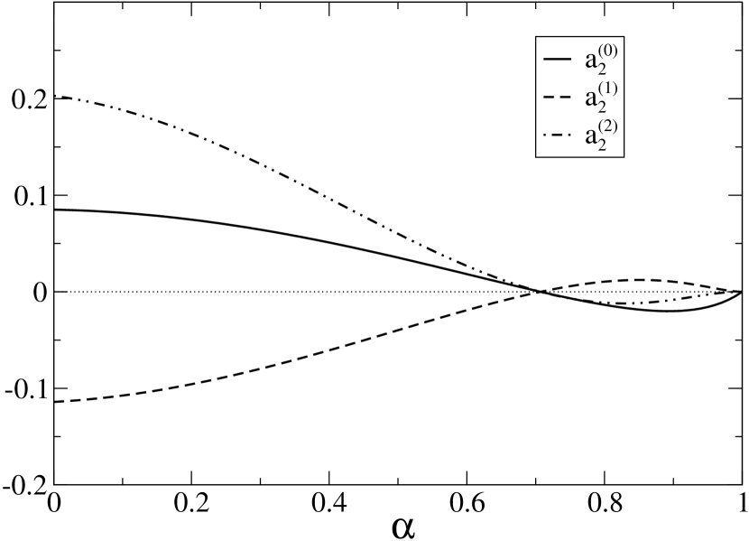
Figure 7: $a_{2}^{(0)}$, $a_{2}^{(1)}$ and $a_{2}^{(2)}$ versus $\alpha$ for $d=2$.

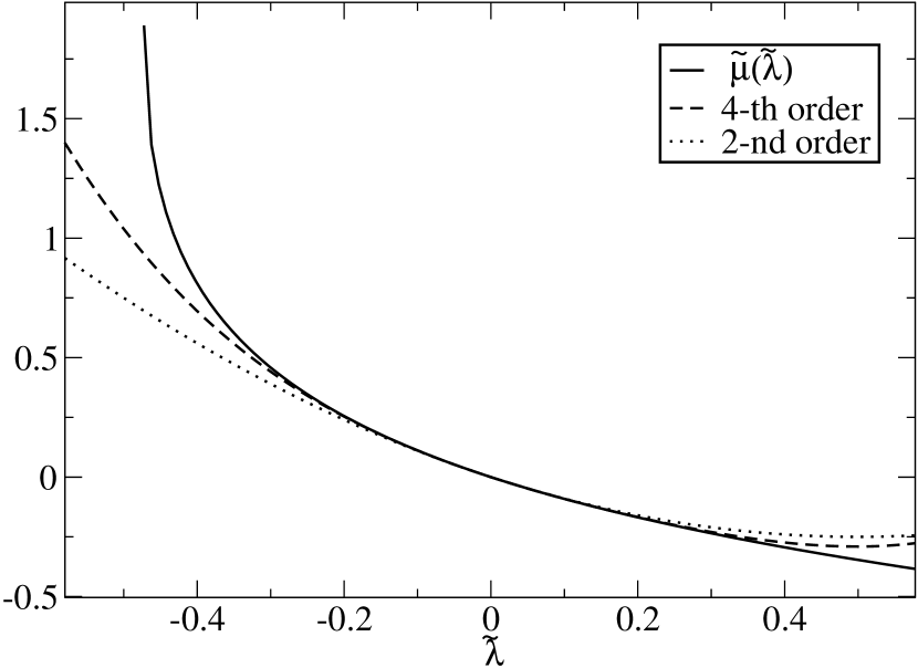
Figure 8: The solid line shows ${\tilde{\mu}}$ in the limit $d\to\infty$. The dashed line is ${\tilde{\mu}}$ at fourth order in ${\tilde{\lambda}}$ from (76) for $d=2$ and $\alpha=0.5$. Finally the dotted line shows the same quantity calculated with a truncation at second order in $\lambda$, which would satisfy the G-C relation.

4.2 The solvable infinite dimension limit

Strong arguments VPB⁺06a can be given showing that in high dimensions ${\tilde{f}}(v,\lambda)$ is not far from a Gaussian. We are therefore led to consider, in the limit $d\to\infty$, ${\tilde{f}}({\bf v},\lambda)$ to be a Gaussian with a $\lambda$-dependent second moment. In this situation the dimensionless function $f$ will read:

$$f({\bf c})={e^{-c^{2}}\over\pi^{d/2}}$$ (91)

with ${\bf c}={\bf v}/v_{0}(\lambda)$. In this context one can solve equation (75) in order to get an explicit expression for $\mu(\lambda)$. Solving the system defined by (75) for $n=0$ and $n=2$ gives a unique solution for ${\tilde{\mu}}({\tilde{\lambda}})$ which verifies the physical requirement ${\tilde{\mu}}(0)=0$:

$${\tilde{\mu}}({\tilde{\lambda}})=-{\tilde{\lambda}}+{{\tilde{\lambda}}^{2}\over 2}{\tilde{v}}_{0}^{2}({\tilde{\lambda}})\,,$$ (92)

with:

$${\tilde{v}}_{0}^{2}({\tilde{\lambda}})=\frac{1+4\,{{\tilde{\lambda}}}^{3}}{2\,{{\tilde{\lambda}}}^{4}}+{b_{1}({\tilde{\lambda}})\over 2}-{1\over 2}\left[-\frac{32}{{{\tilde{\lambda}}}^{2}}+\frac{2\,{\left(1+4\,{{\tilde{\lambda}}}^{3}\right)}^{2}}{{{\tilde{\lambda}}}^{8}}+b_{2}({\tilde{\lambda}})-b_{3}({\tilde{\lambda}})+{b_{4}({\tilde{\lambda}})\over 4b_{1}({\tilde{\lambda}})}\right]^{1\over 2}\,\,,$$ (93)

and

$$\begin{split}b_{1}({\tilde{\lambda}})=\sqrt{{{\tilde{\lambda}}}^{-8}+\frac{8}{{{\tilde{\lambda}}}^{5}}-b_{2}({\tilde{\lambda}})+b_{3}({\tilde{\lambda}})}\,,\quad&b_{2}({\tilde{\lambda}})=\frac{16\,{\left(\frac{2}{3}\right)}^{\frac{1}{3}}}{{{\tilde{\lambda}}}^{3}\,{\left(9+{\sqrt{3}}\,{\sqrt{27+256\,{{\tilde{\lambda}}}^{3}}}\right)}^{\frac{1}{3}}}\,,\\ b_{3}({\tilde{\lambda}})=\frac{2\,{\left(\frac{2}{3}\right)}^{\frac{2}{3}}\,{\left(9+{\sqrt{3}}\,{\sqrt{27+256\,{{\tilde{\lambda}}}^{3}}}\right)}^{\frac{1}{3}}}{{{\tilde{\lambda}}}^{4}}\,,\quad&b_{4}({\tilde{\lambda}})=\frac{256}{{{\tilde{\lambda}}}^{3}}-\frac{192\,\left(1+4\,{{\tilde{\lambda}}}^{3}\right)}{{{\tilde{\lambda}}}^{6}}+\frac{8\,{\left(1+4\,{{\tilde{\lambda}}}^{3}\right)}^{3}}{{{\tilde{\lambda}}}^{12}}\,.\\ \end{split}$$ (94)

This expression of the velocity scale reduces to the kinetic temperature for $\lambda=0$, and decreases monotonically as $\lambda^{-1/2}$ when $\lambda\to\infty$. This means that in the limit $\lambda\to\infty$ ${\tilde{f}}$ approaches a Dirac distribution as $\exp(-\lambda v^{2}/2)$. This feature supports the intuition that the small ${\cal W}$ events (which are related to the large values of $\lambda$) are provided by the small velocities. The behavior of ${\tilde{\mu}}$ is shown in Fig. 8. The large deviations function ${\tilde{\mu}}({\tilde{\lambda}})$ becomes complex for ${\tilde{\lambda}}<-{3\over 2^{8/3}}$, because of the terms containing $\sqrt{27+256{\tilde{\lambda}}^{3}}$. Moreover for large ${\tilde{\lambda}}$ the behavior of this function is ${\tilde{\mu}}({\tilde{\lambda}})\sim-{\tilde{\lambda}}^{1\over 4}$. In the vicinity of the singularity (i.e. ${\tilde{\lambda}}=\lambda_{0}=-{3\over 2^{8/3}}$) the behavior of the large deviation function is:

$${\tilde{\mu}}({\tilde{\lambda}})={3\over 2^{3/2}}-3^{2/3}2^{1/6}\sqrt{{\tilde{\lambda}}-\lambda_{0}}+{\cal O}({\tilde{\lambda}}-\lambda_{0})\,\,.$$ (95)

From the behavior for large ${\tilde{\lambda}}$ it is possible to recover the left tail of the large deviation function $\pi_{\infty}$. In general, if $\mu(\lambda)\sim-\lambda^{\beta}$ for $\lambda\to\infty$, this leads to $\mu^{\prime}(\lambda_{*})=-\beta\lambda_{*}^{\beta-1}=-w$. This last relation tells us that for $\beta<1$ we are recovering the limit $w\to 0^{+}$, with a behavior of the large deviation function given by $\pi_{\infty}(w)=\mu(\lambda_{*})+\lambda_{*}w\sim w^{\beta\over\beta-1}$. Moreover, from the behavior of $\mu$ near $\lambda_{0}$, an analogous calculation provides the right tail of the large deviation function: $\pi_{\infty}(w)\sim\lambda_{0}w$, when $w\to\infty$. Finally, in our particular case, the tails are given by

$${\tilde{\pi}}_{\infty}({\tilde{w}}\to 0^{+})\sim-{\tilde{w}}^{-1/3}\,\,,\,\,{\tilde{\pi}}_{\infty}({\tilde{w}}\to\infty)\sim-{\tilde{w}}\,\,,$$ (96)

Note that there is no $w<0$ tail to ${\tilde{\pi}}_{\infty}$. The graph of the whole function ${\tilde{\pi}}_{\infty}({\tilde{w}})$ is depicted in Fig. 9.

Figure 9: ${\tilde{\pi}}_{\infty}({\tilde{w}})$

5 Fluctuations of injected power at finite times: two examples

5.1 The homogeneous driven gas of inelastic hard disks

In this section the results of numerical simulations of two models (inelastic hard spheres and inelastic Maxwell model) are presented with particular attention to the verification of the Fluctuation Relation for the injected power. The main requirement to pose the question about the validity of the Fluctuation Relation is a clean observation of a negative tail in the pdf of the injected power. This dramatically limits the time $t$ of integration of ${\cal W}(t)$. In numerical simulations, as well as in real experiments, at time larger than a few mean free times the negative tail disappears. On the other hand, at times of the order of $1$-$3$ mean free times, the Fluctuation Relation appears to be correctly verified for the inelastic Hard Spheres model and slightly violated for the inelastic Maxwell model. The measure of the cumulants, anyway, gives a neat indication of the fact that the time of convergence of the large deviation function is at least $10$ times as large and that the true asymptotic is well reproduced by the theory exposed in this chapter. This theory shows strong arguments against the validity of a symmetry relation of the Gallavotti-Cohen type for the large deviations of injected power.

The stationary state of a driven granular gas, modeled by equation (16), under the assumption of Molecular Chaos may be studied with a Direct Simulation Monte Carlo technique Bir (94); MS (00). As a first check of reliability of the algorithm, we have measured the granular temperature $T_{g}$ and the first non-zero Sonine coefficient $a_{2}\equiv(\langle v^{4}\rangle/\langle v^{2}\rangle^{2}-3)/3$. The measured granular temperature is always in perfect agreement with the estimate. The measured $a_{2}$ coefficient is a highly fluctuating quantity and its average is in very good agreement with the theoretical estimate.

In figure 11 the probability density functions $p(w,t)\equiv tP(wt,t)$ (for $t$ equal to $1$ mean free time) for three different choices of parameters $N,\Gamma$ (at fixed restitution coefficient $\alpha$) is shown. The values of the first two cumulants of the distribution and their theoretical values are compared in table 1, with very good agreement. In the same table we present also the measure of the third and fourth cumulants.

N	$\Gamma$	$\langle{\cal W}(t)\rangle/t$	$\langle{\cal W}(t)^{2}\rangle_{c}/t$	$N\Gamma d$	$2N\Gamma dT_{g}$	$\langle{\cal W}(t)^{3}\rangle_{c}/t$	$\langle{\cal W}(t)^{4}\rangle_{c}/t$
100	0.5	100	20835	100	21052	$6.02779\times 10^{5}$	$1.54181\times 10^{8}$
100	12.5	2500	13019125	2500	13157900	$9.47684\times 10^{9}$	$6.12963\times 10^{13}$
200	0.5	199.9	42009	200	42120	$1.21911\times 10^{6}$	$3.09634\times 10^{8}$

Table 1: Rescaled cumulants of the distribution of injected work $P({\cal W},t)$, measured with $t$ equal to $1$ mean free time for different choices of the parameters.

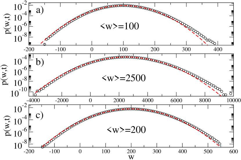
Figure 10: Probability density function of the injected power, $p(w,t)\equiv tP({\cal W}(t)=wt,t)$ with $t$ equal to $1$ mean free time. In all three cases the value of the restitution coefficient is $\alpha=0.9$. Other parameters are a) $N=100$, $\Gamma=0.5$; b) N=100, $\Gamma=12.5$; c) $N=200$, $\Gamma=0.5$. The dashed line represents a Gaussian with same first two cumulants. These distributions have been obtained with $\sim 1.5\times 10^{9}$ independent values of ${\cal W}(t)$.

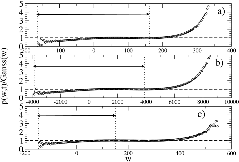
Figure 11: Ratio of $P({\cal W},t)$ and a Gaussian with the same first two moments, for the same parameters as in figure 11: a) corresponds to $N=100$, $\Gamma=0.5$, b) to $N=100$, $\Gamma=12.5$ and c) to $N=200$, $\Gamma=0.5$. The range between the vertical dotted lines is the useful one for the check of the Gallavotti-Cohen relation. It can be noted that the strongest deviations from the Gaussian behavior appear outside of this range.

The comparison with a Gaussian with same mean value and same variance shows that the pdf $P({\cal W},t)$ is not exactly a Gaussian. In particular there are deviations from the Gaussian form in the right (positive) tail. This is well seen in figure 11. It must be noted that the important deviations in the right tail arise at values of ${\cal W}(t)$ larger than the minimum ${\cal W}(t)$ available in the left tail, i.e. they have no influence in the following plot of figure 13 regarding the Gallavotti-Cohen symmetry.

In figure 13 the Gallavotti-Cohen relation $\pi_{t}(w)-\pi_{t}(-w)=\beta_{eff}w$ is questioned for the same choice of the parameters. The relation, at this level of resolution and for this value of the time $t$ ($1$ mean free time), is well satisfied. Moreover table 2 shows that the value of $\beta_{eff}$ is well approximated by $\beta=1/T_{g}$, as expected if the truncation of $\mu(\lambda)$ at the second order were valid, see eq. (79). In figure 13 the same relation is checked for different values of $t$, slightly larger (i.e. up to $t$ equal to $3$ mean free times). No relevant deviations are observed as $t$ is increased. Moreover this figure is important to understand the dramatic consequences that a larger $t$ has on the “visibility” of the Gallavotti-Cohen symmetry: as $t$ is increased, events with negative integrated power injection become rarer and rarer. This eventually leads to the vanishing of the left branch of $P({\cal W},t)$.

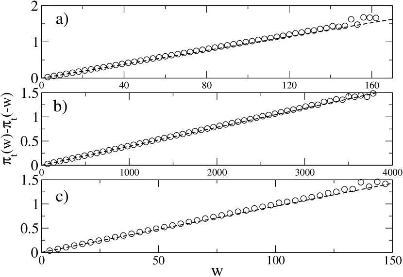
Figure 12: Plot of $\pi_{t}(w)-\pi_{t}(-w)$ vs $w$, for the same choice of the parameters as in figure 11. The values of the slope $\beta_{eff}$ of the fitting dashed lines are in table 2

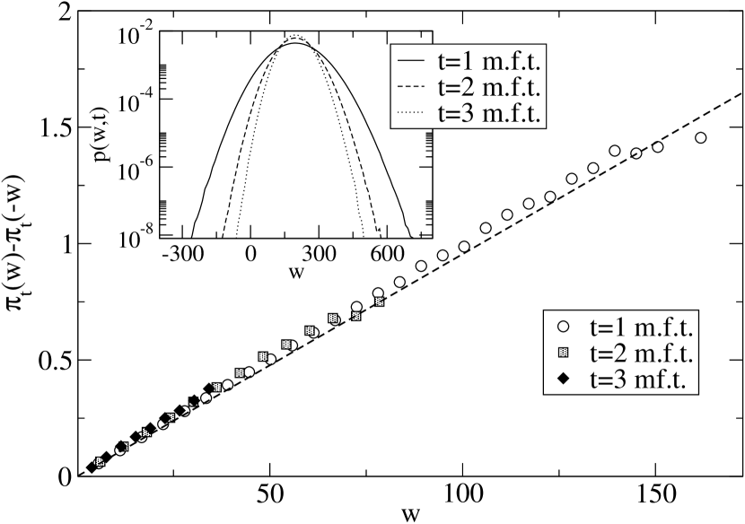
Figure 13: Plot of $\pi_{t}(w)-\pi_{t}(-w)$ versus $w$, for the system with $N=100$ and $\Gamma=0.5$ for different values of $t$. We recall that in this case $\langle w\rangle=100$. The dashed line has slope $\beta=1/T_{g}$. In the inset the corresponding $p(w,t)$ are shown.

N	$\Gamma$	$\beta_{eff}$	$1/T_{g}$
100	0.5	0.0100	0.00955
100	12.5	0.000402	0.000382
200	0.5	0.00995	0.00952

Table 2: Factor of proportionality in the “Gallavotti-Cohen” relation compared with $\beta$.

The main conclusion is that no appreciable departure from the $\lambda^{2}$ truncation is observed at this level of resolution. Much larger statistics are required to probe the very high energy tails of $p(w,t)$. Further numerical insights make evident that the small times used to check the GC Relation ($t$ smaller or equal than $3$ mean free times) are far from the time where the asymptotic large deviation scaling starts working. In figure 15 we show indeed the numerical measure of the third cumulant of ${\cal W}(t)$ rescaled by the first cumulant, varying the integration time $t$. The time of saturation is of the order of $\sim 50$ mean free times. The saturation value is in very good agreement with the value predicted by our theory, eq. (90). Note that this value is not at all trivial, since the third cumulant for a Gaussian distribution is zero. At that time the measurable $\pi_{t}(w)$ is shown in figure 15, rescaled by $\langle w\rangle$. The accessible range of values from a numerical simulation is dramatically poor and we think it is already remarkable to have obtained a good measure of the third cumulant with such a resolution.

The reason for a verification at small times of the GC formula is the following: near $w=0$ the pdf of $w$ is almost a Gaussian. In the Gaussian case we immediately get $\pi_{t}(w)-\pi_{t}(-w)=\beta_{eff}w$ with $\beta_{eff}=2\langle{\cal W}(t)\rangle/\langle{\cal W}(t)^{2}\rangle_{c}$. The first two cumulants at small times are easily obtained considering an uncorrelated sequence of energy injection, obtaining $\langle{\cal W}(t)\rangle/t=N\Gamma d$ and $\langle{\cal W}(t)^{2}\rangle_{c}/t=\langle(\sum_{i}\mathbf{F}_{i}^{th}\cdot\mathbf{v}_{i})^{2}\rangle_{c}=2N\Gamma dT_{g}$. Then the value $\beta_{eff}=1/T_{g}$ is unavoidable. In this case the GCFR observed is nothing else than the Green-Kubo (or Einstein) relation, which is known to be valid for driven granular gases: $\langle{\cal W}(t)^{2}\rangle/t=2T_{g}\langle{\cal W}(t)\rangle/t$ PBL (02); PBV (07). Small deviations from a Gaussian appear, in first approximation, as small deviations from the slope $1/T_{g}$, but the straight line behavior is robust since the first non-linear term of $\pi_{t}(w)-\pi_{t}(-w)$ is not $w^{2}$ but $w^{3}$ AFMP (01).

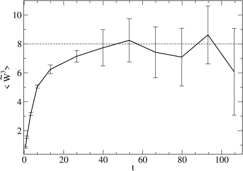
Figure 14: Third cumulant ${\tilde{\cal W}}={\cal W}/(\langle{\cal W}\rangle T_{g}^{2})$ for several times of integration. The time is in units of the mean collision time. Note that the time when a stationary value of the rescaled cumulant is reached is much larger than the characteristic time of the system (the collision time).

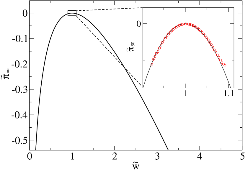
Figure 15: Numerical measurement of ${\tilde{\pi}}_{t}$ for a time of 50 collisions per particle (when a stationary value for the rescaled cumulant is reached).

Numerical simulations of the Inelastic Maxwell Model have been performed with a Direct Simulation Monte Carlo analogous to the one used in the Hard Spheres model. The Maxwell gas is a kinetic model due to Maxwell, who observed that a pair potential proportional to $r^{-2(d-1)}$, $r$ being the distance between two interacting particles, gives rise to a great simplification of the collision integral Max (67). In fact this kind of interaction makes the collision frequency velocity independent. It must be noted that when the inelasticity of the particles is considered, this model looses its straight physical interpretation, but it nevertheless keeps its own interest. The collision integral is analytically simpler than the hard particles model and preserves the essential physical ingredients in order to have qualitatively the same phenomenology. In the recent development of granular gases this kinetic model has been extensively investigated BMP (02); BNK (02, 03); EB (02); BCG (00). Thanks to the simplifications present in this model, we are able to improve the number of collected data by more than a factor of ten. The distributions of the injected power $p(w,t)$ are shown in figure 17 for some choices of the restitution coefficient $\alpha$. The driving amplitude $\Gamma$ has been changed in order to keep constant the stationary granular temperature $T_{g}$. In figure 17 we have displayed the deviations from the Gaussian of $P({\cal W},t)$. The non-Gaussianity of $P({\cal W},t)$ is highly pronounced, but again it is striking only in the positive branch of the pdf. We have tried, with success, a fit with a fourth order polynomial, which is consistent with the usual truncation of the Sonine expansion to the second Sonine polynomial.

Finally, in figure 18, we have attempted a check of the Gallavotti-Cohen fluctuation relation. The relation seems to be systematically violated. This appears in two points: 1) the right-left ratio of the large deviation function is not a straight line; 2) the best fitting line has a slope which is larger than $1/T_{g}$. The “curvature”(and the deviation from the $1/T_{g}$ line) increases with decreasing values of $\alpha$, indicating that the inelasticity is the cause of the deviation from the Gallavotti-Cohen relation. It should be noted that to achieve this result we have collected more than $4\times 10^{10}$ independent values of ${\cal W}(t)$, so that the statistics of the negative large deviations could be clearly displayed.

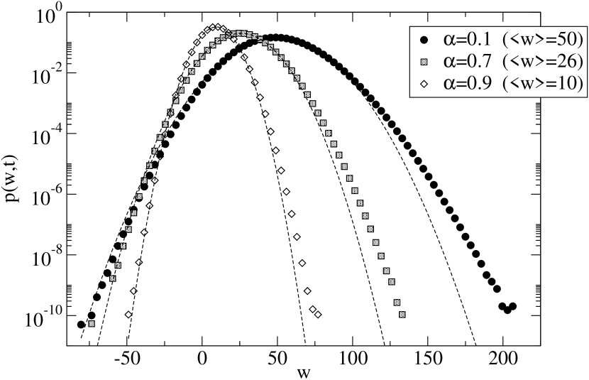
Figure 16: $p(w,t)\equiv tP(wt,t)$ for different values of $\alpha$ (at fixed constant temperature $T_{g}$) in the Driven Inelastic Maxwell Model measured at a time $t$ equal to $1$ mean free time. The dashed lines are Gaussian distributions with the same mean and same variance. These distributions have been obtained with $\sim 4\times 10^{10}$ independent values of ${\cal W}(t)$.

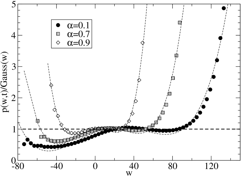
Figure 17: $p(w,t)$ (at $t$ equal to $1$ mean free time) divided by a Gaussian with same average and same variance for different values of $\alpha$ (at fixed constant temperature $T_{g}$) in the Driven Inelastic Maxwell Model. The light dashed lines represent a fit with a polynomial of fourth order.

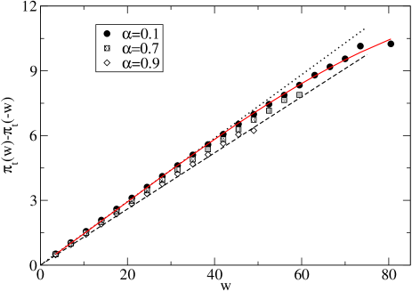
Figure 18: (Color online). Finite time check of Gallavotti-Cohen relation for the injected power (with $t$ equal to $1$ mean free time), i.e. $\pi_{t}(w)-\pi_{t}(-w)$ vs. $w$, in a numerical simulation of the Driven Inelastic Maxwell Model with $N=50$, and different values of $\alpha$ (the driving amplitude $\Gamma$ has been rescaled in order to fix the granular temperature $T_{g}$). The dashed curve is a straight line with slope $\beta=1/T_{g}$. The dotted curve is a straight line obtained fitting the $\alpha=0.1$ data points until $w=45$, useful as a guide for the eye. The thin (red) solid curve is a fit with a cubic ($0.28w+5.6\cdot 10^{-4}w^{2}-1.1\cdot 10^{-5}w^{3}$).

5.2 The boundary driven gas of inelastic hard disks

In a recent experiment on vibrated granular gases FM (04) it has been argued that the statistics of the power injected on a subsystem by the rest of the gas fulfills the Fluctuation Relation (FR) by Gallavotti and Cohen. The experiment was performed by putting in a two-dimensional vertical box $N$ disks of glass and submitting the container to a strong vertical vibration. We have reproduced the experiment by means of a Molecular Dynamics (MD) simulations of inelastic hard disks, observing perfect agreement with the experimental results and obtaining a deeper insight into the system. The main difference of this model with respect to the previous “homogeneously driven” model is that the external energy source is located at the two horizontal (top and bottom) walls. This boundary driving mechanism leads to the development of spatial inhomogeneities and the appearance of internal currents.

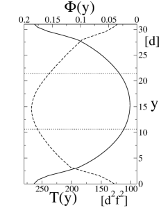
Figure 19: Left: Snapshot of the system considered for MD simulations, with the inner region marked by the solid rectangle. Right: Corresponding vertical profiles of density ($\Phi(y)$, dashed line) and temperature ($T(y)$, solid line). The dotted lines mark the bottom and top boundaries of the inner region. Here $N=270$ and $\alpha=0.9$. The mean free path is $\sim 5.7d$.

The event driven MD simulations have been performed for a system of $N$ inelastic hard disks with restitution coefficient $\alpha$, diameter $\sigma$ and mass $m=1$. The vertical $2D$ box of width $L_{x}=48\sigma$ and height $L_{y}=32\sigma$ is shaken by a sinusoidal vibration with frequency $f$ (period $\tau_{box}=1/f$) and amplitude $2.6\sigma$. Collisions with the elastic walls inject energy and allow the system to reach a stationary state. We have checked that possible inelastic collisions with the walls hardly affect the results. Gravity – set to $g=-1.7\sigma f^{2}$ in order to be consistent with the experiment– has a negligible influence on the measured quantities. We have varied the restitution coefficient from $0.8$ up to $0.99$ (glass beads yield on average $\alpha\approx 0.9$) and the total area coverage from $0.138$ (i.e. $N=270$) up to $0.32$ ($N=620$). In figure 19-left a snapshot of the system is shown. During the simulations the main physical observables are statistically stationary. The local area coverage field $\Phi(x,y)$ and the granular temperature field $T(x,y)$ (defined in $2D$ as the local average kinetic energy per particle) are almost uniform in the horizontal direction, apart from small layers near the side walls. In figure 19-right the profiles $\Phi(y)=(1/L_{x})\int dx\Phi(x,y)$ and $T(y)=(1/L_{x})\int dxT(x,y)$ are shown to be symmetric with respect to the bottom and the top of the box. Following the experimental procedure, we have focused our attention on a “window” in the center of the box, fixed in the laboratory frame, of width $2L_{x}/5$ and height $L_{y}/3$, marked in figure 19-left. Apart from the negligible change of potential energy due to gravity, the total kinetic energy of the particles inside the window, changes during a time $\tau$ because of two contributions: $\Delta K_{\tau}=Q_{\tau}-I_{\tau}$ where $Q_{\tau}$ is the kinetic energy transported by particles through the boundary of the window (summed when going-in and subtracted when going-out) and $I_{\tau}$ is the kinetic energy dissipated in inelastic collisions during time $\tau$. For several values of $\tau$ we have measured, as in the experiments, $Q_{\tau}$ which is related to the kinetic contribution to the heat flux (we checked that inclusion of the collisional contribution, even if non small HMZ (04), does not change the picture). With $N=270$ and $\alpha=0.9$ the characteristic times are the mean free time $\tau_{col}\approx 0.47\tau_{box}$, the diffusion time across the window $\tau_{diff}=0.82\tau_{box}$ and the mean time between two subsequent crossings of particles (from outside to inside) $\tau_{cross}\approx 0.039\tau_{box}$.

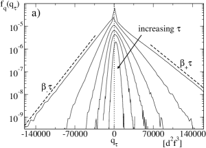
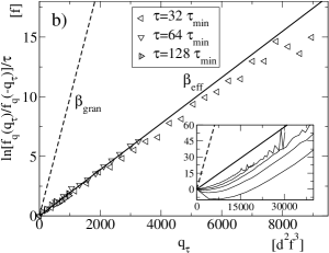
Figure 20: a) pdfs of injected power $f_{q}(q_{\tau})$ from MD simulations for different values of $\tau=(1,2,4,8,16,32)\times\tau_{min}$ with $\tau_{min}=0.015\tau_{box}$. Here $N=270$ and $\alpha=0.9$. The distributions are shifted vertically for clarity. The dashed lines put in evidence the exponential tails of the pdf at $\tau=\tau_{min}$. b) plot of $(1/\tau)\log[f_{q}(q_{\tau})/f_{q}(-q_{\tau})]$ vs. $q_{\tau}$ from MD simulations (same parameters as above) at large values of $\tau$. The solid curve is a linear fit (with slope $\beta_{eff}$) of the data at $\tau=128\tau_{min}$. The dashed line has a slope $\beta_{gran}=1/T_{gran}$. In the inset the same graph is shown for small values of $\tau=(1,2,4,8)\times\tau_{min}$ (from bottom to top).

We define the injected power as $q_{\tau}=Q_{\tau}/\tau$ and two relevant probability density functions (pdfs): $f_{Q}(Q_{\tau})$ and $f_{q}(q_{\tau})$. figure 20a) shows $f_{q}(q_{\tau})$ for different values of $\tau$. A direct comparison with Fig. 3 of Ref. FM (04) suggests a fair agreement between simulations of inelastic hard disks and the experiment. The pdfs are strongly non-Gaussian and asymmetric, becoming narrower as $\tau$ is increased. At small $\tau$ a strong peak in $q_{\tau}=0$ is visible. More interestingly, $f_{q}(q_{\tau})$ at small values of $\tau$ has two different exponential tails, i.e. $f_{q}(q_{\tau})\sim\exp(\mp\beta_{\pm}\tau q_{\tau})$ when $q_{\tau}\to\pm\infty$ with $\beta_{-}>\beta_{+}$. The peak and the exponential tails at small $\tau$ are observed also in the experiment (see Fig. 3 of FM (04)) and in similar simulations AFMP (01). In figure 20b) we display $\log[f_{q}(q_{\tau})/f_{q}(-q_{\tau})]/\tau$ vs. $q_{\tau}$, which is equivalent to the graph of $\pi_{\tau}(q_{\tau})-\pi_{\tau}(-q_{\tau})$ vs. $q_{\tau}$ where $\pi_{\tau}(q_{\tau})=\log[f_{Q}(\tau q_{\tau})]/\tau$. From figure 20 it appears that at large values of $\tau$, $\pi_{\tau}(q_{\tau})-\pi_{\tau}(-q_{\tau})$ is linear with a $\tau$-independent slope $\beta_{eff}\neq 1$. We have measured $\beta_{eff}$ with various choices of the restitution coefficient $\alpha$ and of the covered area fraction finding similar results. Ref. FM (04) reports $\beta_{eff}T_{gran}\sim 0.25$ where $T_{gran}$ is the mean granular temperature in the observation window. Similar values are measured in our MD simulations. At area fraction $13.8\%$ and $\alpha=0.9$ we have $\beta_{eff}T_{gran}\approx 0.23$. At fixed $\alpha$ and increasing area fraction, $\beta_{eff}T_{gran}$ slightly increases, as in the experiment. As $\alpha\to 1$ the slope $\beta_{eff}$ decreases. At $\alpha=1$ (without gravity and external driving) the distribution of $Q_{\tau}$ is symmetrical and $\beta_{eff}=0$, indicating that $1/\beta_{eff}$ is not a physically relevant temperature concept. Interestingly, it appears that $\beta_{eff}$ is a non hydrodynamic quantity: different systems may show the same density and temperature profiles, with very different values of $\beta_{eff}$.

We now adopt a coarse-grained description of the experiment which is able to entirely capture the observed phenomenology. The measured flow of energy is given by

$$Q_{\tau}=\frac{1}{2}\left(\sum_{i=1}^{n_{+}}v_{i+}^{2}-\sum_{i=1}^{n_{-}}v_{i-}^{2}\right),$$ (97)

where $n_{-}$ ($n_{+}$) is the number of particles leaving (entering) the window during the time $\tau$, and $v_{i-}^{2}$ ($v_{i+}^{2}$) are the squared moduli of their velocities. In order to analyze the statistics of $Q_{\tau}$ we take $n_{-}$ and $n_{+}$ as Poisson-distributed random variables with average $\omega\tau$, where $\omega$ corresponds to the inverse of the crossing time $\tau_{cross}$. In doing so we neglect correlations among particles entering or leaving successively the central region. A key point, supported by direct observation in the numerical experiment, lies in the assumption that the velocities ${\bf v}_{i+}$ and ${\bf v}_{i-}$ come from populations with different temperatures $T_{+}$ and $T_{-}$ respectively. Indeed, compared with the population entering the central region, those particles that leave it have suffered on average more inelastic collisions, so that $T_{-}<T_{+}$. Finally we assume Gaussian velocity pdfs. Within such a framework, the distribution $f_{Q}(Q_{\tau})$ of $Q_{\tau}$ can be studied analytically. Here it is enough to recall that $\frac{1}{2}\sum_{i=1}^{n}v_{i}^{2}$, in $D$ dimensions, if each component of ${\bf v}_{i}$ is independently Gaussian-distributed with zero mean and variance $T$, is a stochastic variable $x$ with a distribution $\chi_{n,T}(x)=f_{1/T,Dn/2}(x)$, where $f_{\alpha,\nu}(x)$ is the Gamma distribution, and whose generating function reads $\tilde{\chi}_{n,T}(z)=\left(1-Tz\right)^{-Dn/2}$ Fel (71). It is then straightforward to obtain the generating function of $Q_{\tau}$ in the form $\tilde{f}_{Q}(z)=\exp[\tau\mu(z)]$ with

$$\mu(z)=\omega\left(-2+(1-T_{+}z)^{-D/2}+(1+T_{-}z)^{-D/2}\right).$$ (98)

We observe that $\tilde{f}_{Q}(z)$ has two poles in $z=\pm 1/T_{\pm}$ and two branch cuts on the real axis for $z>1/T_{+}$ and $z<-1/T_{-}$. From $\mu(z)$ we immediately obtain the cumulants of $f_{Q}(Q_{\tau})$ through the formula $\langle Q^{n}\rangle_{c}=\tau\frac{d^{n}}{dz^{n}}\mu(0)$.

For $\tau\to\infty$ the large deviation theory states that $f_{Q}(Q_{\tau})\sim\exp(\tau\pi_{\infty}(Q_{\tau}/\tau))$ and $\pi_{\infty}(q)$ can be obtained from $\mu(z)$ through a Legendre transform, i.e. $\pi_{\infty}(q)=\smash{\underset{z}{max}}(\mu(z)-qz)$. The study of the singularities of $\mu(z)$ reveals the behavior of the large deviation function $\pi_{\infty}(q)$ for $q\to\pm\infty$. It can be seen that

$$\pi_{\infty}(q)\sim-\frac{q}{T_{+}}\;\;(q\to\infty),\;\;\;\pi_{\infty}(q)\sim\frac{q}{T_{-}}\;\;(q\to-\infty).$$ (99)

We emphasize however that it is almost impossible to appreciate these tails in simulations and in experiments, since the statistics for large values of $q$ and $\tau$ is very poor.

A Gallavotti-Cohen-type relation GC (95); LS (99); Kur (98), e.g. $\pi_{\infty}(q)-\pi_{\infty}(-q)=\beta q$ for any $q$ and an arbitrary value of $\beta$ would imply $\mu(z)=\mu(\beta-z)$. One can see that such a $\beta$ does not exist, i.e. the fluctuations of $Q_{\tau}$ do not satisfy a Gallavotti-Cohen-like relation. The observed linearity of the graph $\log[f_{q}(q_{\tau})/f_{q}(-q_{\tau})]/\tau=\pi(q_{\tau})-\pi(-q_{\tau})$ vs. $q_{\tau}$ can be explained by the same observation pointed out in the previous subsection: at large values of $\tau$ it is extremely difficult, in simulations as well as in experiments, to reach large values of $q$, while for small $q$, $\pi(q)-\pi(-q)\approx 2\pi^{\prime}(0)q+o(q^{3})$, i.e. a straight line with a slope $\beta_{eff}=2\pi^{\prime}(0)$ is likely to be observed. It has been already shown Far (02) that in dissipative systems deviations from the FR can be hidden by insufficient statistics at high values of $q$. The knowledge of $\mu(z)$ is useful to predict this slope. At large $\tau$, $\pi^{\prime}(0)\approx\Pi^{\prime}(0)=-z^{*}(0)$ where $z^{*}(q)$ is the value of $z$ for which $\mu(z)-qz$ is extremal. This gives

$$\beta_{eff}=\frac{T_{+}^{\delta}-T_{-}^{\delta}}{T_{+}^{\delta+1}+T_{-}^{\delta+1}}\quad\hbox{with}\quad\delta=\frac{2}{2+D}.$$ (100)

When $T_{+}=T_{-}$ (i.e. if $\alpha=1$) $\beta_{eff}=0$. We emphasize that $\beta_{eff}$ does not depend upon $\omega$. We have compared with success these predictions with the numerical and experimental results, measuring the temperatures $T_{+}$ and $T_{-}$ in the simulation.

What happens for small values of $\tau$? We note that $\tilde{f}_{Q}(z)$ has the form $\exp(\tau\mu(z))$ for any value of $\tau$ and not only for large $\tau$. Therefore at small $\tau$ one can expand the exponential, obtaining $\tilde{f}_{Q}(z)\sim 1+\omega\tau\left(-2+(1-T_{+}z)^{-D/2}+\right.$ $\left.(1+T_{-}z)^{-D/2}\right)$. This immediately leads to an analytical expression for $f_{Q}(Q_{\tau})=\text{const}\times\delta(Q_{\tau})+\chi_{1,T_{+}}(Q_{\tau})+\chi_{1,T_{-}}(-Q_{\tau})$, which fairly accounts for the strong peak which is observed in the experiment and in the simulations, and predicts exponential tails for $f_{Q}(Q_{\tau})$: $\chi_{1,T}(x)\propto x^{D/2-1}\exp(-x/T)$ so that $\beta_{+}=1/T_{+}$ and $\beta_{-}=1/T_{-}$. This suggests an experimental test of this theoretical approach: the measure at small values of $\tau$ of the slopes of the exponential tails of $f_{Q}(Q_{\tau})$ should coincide with a direct measure of $T_{+}$ and $T_{-}$. However, we point out that the values of $\beta_{+}$ and $\beta_{-}$ obtained by fitting the tails in the hard disks simulation, using values as small as $\tau=0.00015\tau_{box}$ yield estimates of $T_{+}$ and $T_{-}$ which are larger (by a factor $\sim 1.6$) than those found by a direct measure. This disagreement brings the limits of such a simple two-temperature picture to the fore. In the simulation and in the original experiment the measured injected energy is indeed the sum of several different contributions, namely $Q_{\tau}\approx Q_{\tau}^{xx}+Q_{\tau}^{xy}+Q_{\tau}^{yx}+Q_{\tau}^{yy}$ where $Q_{\tau}^{ij}$ is the kinetic energy transported by the $i$ component of the velocity by particles crossing the boundary through a wall perpendicular to direction $j$. Two main differences with the simplified interpretation given above arise: a) there are two couples of temperatures, i.e. $T_{+}^{x},T_{-}^{x}$ as well as $T_{+}^{y},T_{-}^{y}$ BC (98); ML (98); BK (03); b) the diagonal contributions $Q_{\tau}^{jj}$ are sums of squares of velocities whose distribution is not a Gaussian but is $\sim v\exp(-v^{2}/T)$, since the probability of crossing is biased by the velocity itself. The calculation of $f_{Q}(Q_{\tau})$ is still feasible, with qualitatively similar results.

6 The dynamics of a tracer particle as a non-equilibrium Markov process

In the search for a quantity that is, more rigorously, related to the “entropy production” in a granular gas, we consider in this section the projection of the dynamics of the gas onto that of a tracer particle, which is easier since it is equivalent to a jump Markov process. We are interested in the dynamics of a tracer granular particle in a homogeneous and dilute gas of grains which is driven by an unspecified energy source. The requirements are that the gas is dilute, spatially homogeneous and time translational invariant. The gas is characterized by its velocity probability density function $P(\mathbf{v})$ which, for the sake of simplicity, will be considered of the form $P(\mathbf{v})=\frac{1}{(2\pi T)^{d/2}}\exp{\left(-\frac{v^{2}}{2T}\right)}(1+a_{2}S_{2}^{d}(v^{2}/2T))$, (where $S_{2}^{d}$ is the $d$-dimensional second Sonine polynomial already defined in 2.2). The gas is therefore parametrized by its temperature $T$ and its second Sonine coefficient $a_{2}$ which measures its non-Gaussianity.

The linear Boltzmann equation for the tracer, in generic dimension $d$, reads:

$$\frac{\textrm{d}P_{*}(\mathbf{v},t)}{\textrm{d}t}=\frac{1}{\ell}\int\textrm{d}\mathbf{v}_{1}\int\textrm{d}\mathbf{v}_{2}\int^{\prime}\textrm{d}\hat{\boldsymbol{\omega}}|(\mathbf{v}_{1}-\mathbf{v}_{2})\cdot\hat{\boldsymbol{\omega}}|P_{*}(\mathbf{v}_{1})P(\mathbf{v}_{2})\times\\ \times\left\{\delta\left(\mathbf{v}-\mathbf{v}_{1}+\frac{1+\alpha}{2}[(\mathbf{v}_{1}-\mathbf{v}_{2})\cdot\hat{\boldsymbol{\omega}}]\hat{\boldsymbol{\omega}}\right)-\delta(\mathbf{v}-\mathbf{v}_{1})\right\}$$ (101)

where $P_{*}(v)$ is the velocity pdf of the test particle and the primed integral again indicates that the integration is performed on all angles that satisfy $(\mathbf{v}_{1}-\mathbf{v}_{2})\cdot\hat{\boldsymbol{\omega}}>0$. The mean free path $\ell$ appears in front of the collision integrals. In the following (when not stated differently) we will put $\ell=1$, which can be always obtained by a rescaling of time.

We rewrite the above equation (101) as a Master equation for a Markov jump process PVTvW (06):

$$\frac{\textrm{d}P_{*}(\mathbf{v},t)}{\textrm{d}t}=\int\textrm{d}\mathbf{v}_{1}P_{*}(\mathbf{v}_{1})K(\mathbf{v}_{1},\mathbf{v})-\int\textrm{d}\mathbf{v}_{1}P_{*}(\mathbf{v})K(\mathbf{v},\mathbf{v}_{1}).$$ (102)

The transition rate $K(\mathbf{v},\mathbf{v}^{\prime})$ of jumping from $\mathbf{v}$ to $\mathbf{v}^{\prime}$ is given by the following formula:

$$K({\bf v},{\bf v}^{\prime})=\left(\frac{2}{1+\alpha}\right)^{2}\frac{1}{\ell}|\Delta{\bf v}|^{2-d}\int\textrm{d}{\bf v}_{2\tau}P[\mathbf{v}_{2}(\mathbf{v},\mathbf{v}^{\prime},{\bf v}_{2\tau})],$$ (103)

where $\Delta{\bf v}={\bf v}^{\prime}-{\bf v}$ denotes the change of velocity of the test particle after a collision. The vectorial function ${\bf v}_{2}$ is defined as

$$\mathbf{v}_{2}(\mathbf{v},\mathbf{v}^{\prime},{\bf v}_{2\tau})=v_{2\sigma}(\mathbf{v},\mathbf{v}^{\prime})\hat{\boldsymbol{\sigma}}(\mathbf{v},\mathbf{v}^{\prime})+{\bf v}_{2\tau},$$ (104)

where $\hat{\boldsymbol{\sigma}}(\mathbf{v},\mathbf{v}^{\prime})$ is the unitary vector parallel to $\Delta{\bf v}$, while ${\bf v}_{2\tau}$ is entirely contained in the $(d-1)$-dimensional space perpendicular to $\Delta{\bf v}$ (i.e. ${\bf v}_{2\tau}\cdot\Delta{\bf v}=0$). This implies that the integral in expression (103) is $(d-1)$-dimensional. Finally, to fully determine the transition rate (103), the expression of $v_{2\sigma}$ is needed:

$$v_{2\sigma}({\bf v},{\bf v}^{\prime})=\frac{2}{1+\alpha}|\Delta{\bf v}|+{\bf v}\cdot\hat{\boldsymbol{\sigma}}\,\,\,.$$ (105)

6.1 Detailed balance

Here, we obtain a simple expression for the ratio between $K(\mathbf{v},\mathbf{v}^{\prime})$ and $K(\mathbf{v}^{\prime},\mathbf{v})$. When exchanging $\mathbf{v}$ with $\mathbf{v}^{\prime}$ the unitary vector $\hat{\boldsymbol{\sigma}}$ changes sign. Furthermore one has that $v_{2\sigma}({\bf v},{\bf v}^{\prime})\neq v_{2\sigma}({\bf v}^{\prime},{\bf v})$. From all these considerations and from equation (103) one obtains immediately:

$$\frac{K(\mathbf{v},\mathbf{v}^{\prime})}{K(\mathbf{v}^{\prime},\mathbf{v})}=\frac{\int\textrm{d}{\bf v}_{2\tau}P[\mathbf{v}_{2}({\bf v},{\bf v}^{\prime})]}{\int\textrm{d}{\bf v}_{2\tau}P[\mathbf{v}_{2}({\bf v}^{\prime},{\bf v})]}\equiv\frac{P[v_{2\sigma}({\bf v},{\bf v}^{\prime})]}{P[v_{2\sigma}({\bf v}^{\prime},{\bf v})]}\,\,\,.$$ (106)

We note that this ratio depends only on the choice of the pdf of the gas, $P$, and not on the other parameters (such as $\alpha$). However in realistic situations (experiments or Molecular Dynamics simulations) $P$ is not a free parameter but is determined by the choice of the setup (e.g. external driving, material details, geometry of the container, etc.).

Introducing the short-hand notation $v_{2\sigma}=v_{2\sigma}({\bf v},{\bf v}^{\prime})$, $v_{2\sigma}^{\prime}=v_{2\sigma}({\bf v}^{\prime},{\bf v})$ and $v_{\sigma}^{(\prime)}={\bf v}^{(\prime)}\cdot\hat{\boldsymbol{\sigma}}$, we also note that

$$(v_{2\sigma}^{\prime})^{2}=v_{2\sigma}^{2}+(v_{\sigma}+v_{\sigma}^{\prime})^{2}-2v_{2\sigma}(v_{\sigma}+v_{\sigma}^{\prime})\,\,,$$ (107)

from which it follows that

$$\Delta_{2}=(v_{2\sigma})^{2}-(v_{2\sigma}^{\prime})^{2}=-\Delta-2\frac{1-\alpha}{1+\alpha}\Delta=-\frac{3-\alpha}{1+\alpha}\Delta\,\,,$$ (108)

where $\Delta=v_{\sigma}^{2}-(v_{\sigma}^{\prime})^{2}\equiv|v|^{2}-|v^{\prime}|^{2}$, i.e. the kinetic energy lost by the test-particle during one collision. When $\alpha=1$ then $\Delta_{2}=-\Delta$ (energy conservation). From the above considerations it follows that

• in the Gaussian case, it is found

  $$\log\frac{K(\mathbf{v},\mathbf{v}^{\prime})}{K(\mathbf{v}^{\prime},\mathbf{v})}=\frac{\Delta}{2T}+2\frac{1-\alpha}{1+\alpha}\frac{\Delta}{2T}=\frac{3-\alpha}{1+\alpha}\frac{\Delta}{2T}$$ (109)

• in the First Sonine Correction case, it is found

  $$\log\frac{K(\mathbf{v},\mathbf{v}^{\prime})}{K(\mathbf{v}^{\prime},\mathbf{v})}=\frac{3-\alpha}{1+\alpha}\frac{\Delta}{2T}+\log\frac{\left\{1+a_{2}S_{2}^{d=1}\left[\frac{\left(\frac{2}{1+\alpha}(v_{\sigma}^{\prime}-v_{\sigma})+v_{\sigma}\right)^{2}}{2T}\right]\right\}}{\left\{1+a_{2}S_{2}^{d=1}\left[\frac{\left(\frac{2}{1+\alpha}(v_{\sigma}-v_{\sigma}^{\prime})+v_{\sigma}^{\prime}\right)^{2}}{2T}\right]\right\}}$$ (110)

In the case where $P(v)$ is a Gaussian with temperature $T$, it is immediate to observe that

$$P_{*}(\mathbf{v})K(\mathbf{v},\mathbf{v}^{\prime})=P_{*}(\mathbf{v}^{\prime})K(\mathbf{v}^{\prime},\mathbf{v})$$ (111)

if $P_{*}$ is equal to a Gaussian with temperature $T^{\prime}=\frac{\alpha+1}{3-\alpha}T\leq T$. This means that there is a Gaussian stationary solution of equation (102) (in the Gaussian-bulk case), which satisfies detailed balance. The fact that such a Gaussian with a different temperature $T^{\prime}$ is an exact stationary solution was known from MP (99). It thus turns out that detailed balance is satisfied, even out of thermal equilibrium. Of course this is an artifact of such a model: it is highly unrealistic that a granular gas yields a Gaussian velocity pdf. As soon as the gas velocity pdf $P(v)$ ceases to be Gaussian, detailed balance is violated, i.e. the stationary process performed by the tracer particle is no more in equilibrium within the thermostatting gas. We will see in section 6.2 how to characterize this departure from equilibrium.

6.2 Action functionals

From the previous section we have learnt that the dynamics of the velocity of a tracer particle immersed in a granular gas is equivalent to a Markov process with well defined transition rates. This means that the velocity of the tracer particle stays in a state $\mathbf{v}$ for a random time $t\geq 0$ distributed with the law $r(\mathbf{v})e^{-r(\mathbf{v})t}\textrm{d}t$ and then makes a transition to a new value $\mathbf{v}^{\prime}$ with a probability $r(\mathbf{v})^{-1}K(\mathbf{v},\mathbf{v}^{\prime})$, with $r(\mathbf{v})=\int\textrm{d}\mathbf{v}^{\prime}K(\mathbf{v},\mathbf{v}^{\prime})$. At this point it is interesting to ask about some characterization of the non-equilibrium dynamics, i.e. of the violation of detailed balance, which we know to happen whenever the surrounding granular gas has a non-Gaussian distribution of velocity.

To this extent, we define two different action functionals, following LS (99):

$$W(t) =\sum_{i=1}^{n(t)}\log\frac{K(\mathbf{v}_{i}\to\mathbf{v}_{i}^{\prime})}{K(\mathbf{v}_{i}^{\prime}\to\mathbf{v}_{i})}$$ (112a)

$$\overline{W}(t) =\log\frac{P_{*}(\mathbf{v}_{1})}{P_{*}(\mathbf{v}_{n(t)}^{\prime})}+\sum_{i=1}^{n(t)}\log\frac{K(\mathbf{v}_{i}\to\mathbf{v}_{i}^{\prime})}{K(\mathbf{v}_{i}^{\prime}\to\mathbf{v}_{i})}$$ (112b)

$$\equiv\log\frac{\mathcal{P}(\mathbf{v}_{1}\to\mathbf{v}_{2}\to...\to\mathbf{v}_{n(t)})}{\mathcal{P}(\mathbf{v}_{n(t)}\to\mathbf{v}_{n(t)-1}\to...\to\mathbf{v}_{1})}$$ (112c)

where $i$ is the index of collision suffered by the tagged particle, $\mathbf{v}_{i}$ is the velocity of the particle before the $i$-th collision, $\mathbf{v}_{i}^{\prime}$ is its post-collisional velocity, $n(t)$ is the total number of collisions in the trajectory from time $0$ up to time $t$, and $K$ is the transition rate of the jump due to the collision. Finally, we have used the notation $\mathcal{P}(\mathbf{v}_{1}\to\mathbf{v}_{2}\to...\to\mathbf{v}_{n})$ to identify the probability of observing the trajectory $\mathbf{v}_{1}\to\mathbf{v}_{2}\to...\to\mathbf{v}_{n}$. The quantities $W(t)$ and $\overline{W}(t)$ are different for each different trajectory (i.e. sequence of jumps) of the tagged particle. Note that the first term $\log\frac{P_{*}(\mathbf{v}_{1})}{P_{*}(\mathbf{v}_{n(t)}^{\prime})}$ in the definition of $\overline{W}(t)$, eq. (112c), is non-extensive in time. The two above functionals have the following properties:

• $W(t)\equiv 0$ if there is exact symmetry, i.e. if $K(\mathbf{v}_{i}\to\mathbf{v}_{i+1})=K(\mathbf{v}_{i+1}\to\mathbf{v}_{i})$ (e.g. in the microcanonical ensemble); $\overline{W}(t)\equiv 0$ if there is detailed balance (e.g. any equilibrium ensemble);

• we expect that, for large enough $t$, for almost all the trajectories $\lim_{s\to\infty}W(s)/s=\lim_{s\to\infty}\overline{W}(s)/s=\langle W(t)/t\rangle=\langle\overline{W}(t)/t\rangle$; here (since the system under investigation is ergodic and stationary) the meaning of $\langle\rangle$ is intuitively an average over many independent segments of a single very long trajectory;

• for large enough $t$: 1) at equilibrium $\langle W(t)\rangle=\langle\overline{W}(t)\rangle=0$; 2) out of equilibrium (i.e. if detailed balance is not satisfied) those two averages are positive; we use those equivalent averages, at large $t$, to characterize the distance from equilibrium of the stationary system;

• if $S(t)=-\int\textrm{d}vP_{*}(v,t)\log P_{*}(v,t)$ is the entropy associated to the pdf of the velocity of the tagged particle $P_{*}(v,t)$ at time $t$ (e.g. $-H$ where $H$ is the Boltzmann-H function), then

  $$\frac{\textrm{d}}{\textrm{d}t}S(t)=R(t)-A(t)$$ (113)

  where $R(t)$ is always non-negative, $A(t)$ is linear with respect to $P_{*}$ and, finally, $\langle W(t)\rangle\equiv\int_{0}^{t}\textrm{d}t^{\prime}A(t^{\prime})$. This leads to consider $W(t)$ equivalent to the contribution of a single trajectory to the total entropy flux. In a stationary state $A(t)=R(t)$ and therefore the flux is equivalent to the production; this property has been recognized in LS (99).

• $FR_{W}$ (Lebowitz-Spohn-Gallavotti-Cohen fluctuation relation): $\pi(w)-\pi(-w)=w$ where $\pi(w)=\lim_{t\to\infty}\frac{1}{t}\log{f_{W}^{t}(tw)}$ and $f_{W}^{t}(x)$ is the probability density function of finding $W(t)=x$ at time $t$; at equilibrium the $FR_{W}$ has no content; note that in principle $\pi^{\prime}(w,t)=\frac{1}{t}\log{f_{W}^{t}(tw)}\neq\pi(w)$ at any finite time; a generic derivation of this property has been obtained in LS (99), while a rigorous proof with more restrictive hypothesis is in Mae (99); the discussion for the case of a Langevin equation is in Kur (98).

• $FR_{\overline{W}}$ (Evans-Searles fluctuation relation): $\overline{\pi}(w,t)-\overline{\pi}(-w,t)=w$ where $\overline{\pi}(w,t)=\frac{1}{t}\log{f_{\overline{W}}^{t}(tw)}$ and $f_{\overline{W}}^{t}(x)$ is the probability density function of finding $\overline{W}(t)=x$ at time $t$; at equilibrium the $FR_{\overline{W}}$ has no content; this relation is derived in LS (99); the analogy between this relation and the Evans-Searles fluctuation relation ES (94, 02) has been put forward in PVTvW (06)

A detailed numerical study PVTvW (06) of the fluctuations of $W(t)$ and $\overline{W}(t)$ in this model has shown on the one hand that, out of equilibrium (i.e. when the surrounding gas is non-Gaussian), the $FR_{\overline{W}}$ is always satisfied. On the other hand the $FR_{W}$ is always violated, even if it was expected on the basis of the arguments given in LS (99). The difference between the two functionals defined in (112) is a term which is non-extensive in time, but which has fluctuations whose distribution has exponential tails and therefore, in principle, can contribute to the large deviation function of $W(t)$ PRV (06); Vis (06). Such a failure of a large time Fluctuation Relation, which is much more pronounced in the near-to-equilibrium cases, is similar to that observed in other systems ESR (05); Far (02); vZC (03); BGGZ (05)

7 Conclusions

The study of the fluctuations of global physical quantities in a granular gas is at its very beginning. In the lack of a general rigorous theory in the framework of non equilibrium statistical mechanics, experiments and numerical simulations are the main source of results, together with few exact analytical calculations. In this review of recent results VPB⁺ (05); PVB⁺ (05); VPB⁺06a ; PVTvW (06); VPB⁺06b we have indicated some routes that have been followed, focusing on two global quantities (total energy and energy injection rate) that are of interest in nowadays physics of non-equilibrium systems BHP (98); BdSMRM (05); AFMP (01); AFFM (04); Far (02, 04). On one hand we have shown that total energy fluctuations have a pdf that strongly depends on the model considered. We have also pointed out that definitive inferences about the presence of correlations, starting from the observation of “anomalous” pdfs of total energy, must be drawn with caution, since the lack of spatial or temporal translational invariance may play a major role. On the other hand we have presented a method to calculate the large deviation function of injected power in a granular gas: this method strongly suggests the disappearance of a negative branch in such large deviation function. This result is a direct consequence of the time-irreversibility of inelastic collisions: injected power fluctuations are dominated at large times by the energy dissipated in collisions, which is always positive. Finally we have sketched a recipe to obtain a quantity related to time-reversal asymmetry (i.e. violation of detailed balance) whose large deviations can be both positive and negative. This quantity has the advantage of being measurable in experiments, but the disadvantage of not having an obvious “macroscopic” counterpart. It contains in fact information on the non-Gaussianity of the velocity pdf of the gas. This consideration is in our opinion the main open issue in this study.

References

- AFFM [04] S. Aumaître, J. Farago, S. Fauve, and S. McNamara. Energy and poweer fluctuations in vibrated granular gases. Eur. Phys. J. B, 42:255, 2004.
- AFMP [01] S. Aumaître, S. Fauve, S. McNamara, and P. Poggi. Power injected in dissipative systems and the fluctuation theorem. Eur. Phys. J. B, 19:449–460, 2001.
- BC [98] J. J. Brey and D. Cubero. Steady state of a fluidized granular medium between two walls at thesame temperature. Phys. Rev. E, 57(2):2019–2029, 1998.
- BC [01] J. J. Brey and D. Cubero. Hydrodynamic transport coefficients of granular gases. In T. Pöschel and S. Luding, editors, Granular Gases, pages 59–79, Berlin, 2001. Springer.
- BCG [00] A. V. Bobylev, J. A. Carrillo, and I. M. Gamba. On some properties of kinetic and hydrodynamic equations for inelastic interactions. J. Stat. Phys., 98:743, 2000.
- BDKS [98] J. J. Brey, J. W. Dufty, C. S. Kim, and A. Santos. Hydrodynamics for granular flow at low density. Phys. Rev. E, 58(4):4638, 1998.
- BdSMRM [04] J.J. Brey, M.I.G. de Soria, P. Maynar, and M.J. Ruiz-Montero. Energy fluctuations in the homogeneous cooling state of granular gases. Phys. Rev. E, 70(011302), 2004.
- BdSMRM [05] J.J. Brey, M.I.G. de Soria, P. Maynar, and M.J. Ruiz-Montero. Scaling and universality of critical fluctuations in granular gases. Phys. Rev. Lett., 94:098001, 2005.
- Ber [05] E. Bertin. Global fluctuations and gumbel statistics. cond-mat/0506166, to appear on Phys. Rev. Lett., 2005.
- BGGZ [05] F. Bonetto, G. Gallavotti, A. Giuliani, and F. Zamponi. Chaotic hypothesis, fluctuation theorem and singularities. cond-mat/0507672, 2005.
- BHP [98] S. T. Bramwell, P. C. W. Holdsworth, and J.-F. Pinton. Universality of rare fluctuations in turbulence and critical phenomena. Nature, 396:552–554, 1998.
- Bir [94] G. A. Bird. Molecular Gas Dynamics and the Direct Simulation of Gas Flows. Clarendon, Oxford, 1994.
- BK [03] D. L. Blair and A. Kudrolli. Collision statistics of driven granular materials. Phys. Rev. E, 67:041301, 2003.
- BMP [02] A. Baldassarri, U. Marini Bettolo Marconi, and A. Puglisi. Influence of correlations on the velocity statistics of scalar granular gases. Europhys. Lett., 58:14–20, 2002. cond-mat/0111066.
- BNK [02] E. Ben-Naim and P. L. Krapivsky. Nontrivial velocity distributions in inelastic gases. J. Phys. A: Math. Gen., 35:L147–L152, 2002. cond-mat/0111044.
- BNK [03] E. Ben-Naim and P.L. Krapivsky. The inelastic maxwell model. In Lecture Notes in Physics, volume 624, page 65, Berlin, 2003. Springer. cond-mat/0301238.
- BRMM [00] J. Javier Brey, M. J. Ruiz-Montero, and F. Moreno. Boundary conditions and normal state for a vibrated granular fluid. Phys. Rev. E, 62:5339–5346, 2000.
- BT [02] A. Barrat and E. Trizac. Molecular dynamics simulations of vibrated granular gases. Phys. Rev. E, 66(5):051303, 2002. cond-mat/0207267.
- BTE [05] A. Barrat, E. Trizac, and M. H. Ernst. Granular gases: dynamics and collective effects. J. Phys. Condens. Matter, 17:S2429, 2005.
- CC [60] S. Chapman and T. G. Cowling. The mathematical theory of nonuniform gases. Cambridge University Press, London, 1960.
- CDPT [03] F. Coppex, M. Droz, J. Piasecki, and E. Trizac. On the first sonine correction for granular gases. Physica A, 329:114, 2003.
- CPM [07] G. Costantini, A. Puglisi, and U. Marini Bettolo Marconi. Velocity fluctuations in a one dimensional inelastic Maxwell model. J. Stat. Mech., page P08031, 2007.
- dGM [69] S. R. de Groot and P. Mazur. Non-equilibrium thermodynamics. North-Holland, Amsterdam, 1969.
- EB [02] M. H. Ernst and R. Brito. High-energy tails for inelastic maxwell models. Europhys. Lett., 58:182, 2002.
- EC [81] M. H. Ernst and E. G. D. Cohen. Nonequilibrium fluctuations in -space. J. Stat. Phys, 25(1):153, 1981.
- ECM [93] D. J. Evans, E. G. D. Cohen, and G. P. Morriss. Probability of second law violations in shearing steady states. Phys. Rev. Lett., 71:2401, 1993.
- ES [94] D. J. Evans and D. J. Searles. Equilibrium microstates which generate second law violating steady states. Phys. Rev. E, 50:1645, 1994.
- ES [02] D. J. Evans and D. J. Searles. The fluctuation theorem. Adv. Phys., 51:1529, 2002.
- ESR [05] D. J. Evans, D. J. Searles, and L. Rondoni. Application of the gallavotti-cohen fluctuation relation to thermostated steady states near equilibrium. Phys. Rev. E, 71:056120, 2005.
- Far [02] J. Farago. Injected power fluctuations in langevin equation. J. Stat. Phys., 107:781, 2002.
- Far [04] J. Farago. Power fluctuations in stochastic models of dissipative systems. Physica A, 331:69–89, 2004.
- Fel [71] W. Feller. Probability Theory and its Applications. John Wiley & Sons, New York, 1971.
- FM [04] K. Feitosa and N. Menon. Fluidized granular medium as an instance of the fluctuation theorem. Phys. Rev. Lett, 92:164301, 2004.
- GC [95] G. Gallavotti and E. G. D. Cohen. Dynamical ensembles in nonequilibrium statistical mechanics. Phys. Rev. Lett., 74:2694, 1995.
- GZBN [97] E. L. Grossman, T. Zhou, and E. Ben-Naim. Towards granular hydrodynamics in two-dimensions. Phys. Rev. E, 55:4200, 1997.
- HBB [00] C. Henrique, G. Batrouni, and D. Bideau. Diffusion as mixing mechanism in granular materials. Phys. Rev. E, 63:011304, 2000. cond-mat/0003354.
- HMZ [04] O. Herbst, P. M. Müller, and A. Zippelius. Local heat flux and energy loss in a 2d vibrated granular gas. cond-mat/0412334, 2004.
- Kum [98] V. Kumaran. Temperature of a granular material “fluidized” by external vibrations. Phys. Rev. E, 57(5):5660–5664, 1998.
- Kur [98] J. Kurchan. Fluctuation theorem for stochastic dynamics. J. Phys. A., 31:3719, 1998.
- LS [99] J. L. Lebowitz and H. Spohn. A gallavotti-cohen-type symmetry in the large deviation functional for stochastic dynamics. J. Stat. Phys., 95:333, 1999.
- Mae [99] C. Maes. The fluctuation theorem as a gibbs property. J. Stat. Phys., 95:367, 1999.
- Max [67] J. C. Maxwell. On the dynamical theory of gases. Phil. Trans., 157:49, 1867.
- MB [97] S. McNamara and J.-L. Barrat. The energy flux into a fluidized granular medium at a vibrating wall. Phys. Rev. E, 55:7767, 1997.
- ML [98] S. McNamara and S. Luding. Energy flows in vibrated granular media. Phys. Rev. E, 58:813–822, 1998.
- MP [99] P. A. Martin and J. Piasecki. Thermalization of a particle by dissipative collisions. Europhys. Lett., 46(5):613, 1999.
- MS [00] José Maria Montanero and Andrés Santos. Computer simulation of uniformly heated granular fluids. Granular Matter, 2(2):53–64, 2000. cond-mat/0002323.
- MSS [01] S. J. Moon, M. D. Shattuck, and J. B. Swift. Velocity distribution and correlations in homogeneously heated granular media. Phys. Rev. E, 64:031303, 2001. cond-mat/0105322.
- PBL [02] A. Puglisi, A. Baldassarri, and V. Loreto. Fluctuation-dissipation relations in driven granular gases. Phys. Rev. E, 66:061305, 2002. cond-mat/0206155.
- PBV [07] A. Puglisi, A. Baldassarri, and A. Vulpiani. Violation of the Einstein relation in granular fluids: the role of correlations. J. Stat. Mech., page P08016, 2007.
- PLM+ [98] A. Puglisi, V. Loreto, U. M. B. Marconi, A. Petri, and A. Vulpiani. Clustering and non-gaussian behavior in granular matter. Phys. Rev. Lett., 81:3848, 1998.
- PO [98] G. Peng and T. Ohta. Steady state properties of a driven granular medium. Phys. Rev. E, 58:4737–46, 1998. cond-mat/9710119.
- PRV [06] A. Puglisi, L. Rondoni, and A. Vulpiani. Relevance of initial and final conditions for the fluctuation relation in Markov processes. J. Stat. Mech., page P08010, 2006.
- PTvNE [02] I. Pagonabarraga, E. Trizac, T. P. C. van Noije, and M. H. Ernst. Randomly driven granular fluids: Collisional statistics and short scale structure. Phys. Rev. E, 65(1):011303, 2002.
- PVB+ [05] A. Puglisi, P. Visco, A. Barrat, E. Trizac, and F. van Wijland. Fluctuations of internal energy flow in a vibrated granular gas. Phys. Rev. Lett., 95:110202, 2005.
- PVTvW [06] A. Puglisi, P. Visco, E. Trizac, and F. van Wijland. Dynamics of a tracer granular particle as a non-equilibrium markov process. Phys. Rev. E, 73:021301, 2006.
- Vis [06] P. Visco. Work fluctuations for a Brownian particle between two thermostats. J. Stat. Mech., page P06006, 2006.
- vNE [98] T. P. C. van Noije and M. H. Ernst. Velocity distributions in homogeneously cooling and heated granular fluids. Granular Matter, 1(2):57–64, 1998.
- vNETP [99] T. P. C. van Noije, M. H. Ernst, E. Trizac, and I. Pagonabarraga. Randomly driven granular fluids: Large scale structure. Phys. Rev. E, 59:4326–4341, 1999.
- VPB+ [05] P. Visco, A. Puglisi, A. Barrat, E. Trizac, and F. van Wijland. Injected power and entropy flow in a heated granular gas. Europhys. Lett., 72:55–61, 2005.
- [60] P. Visco, A. Puglisi, A. Barrat, E. Trizac, and F. van Wijland. Fluctuations of power injection in randomly driven granular gases. J. Stat. Phys., 125:529–564, 2006.
- [61] P. Visco, A. Puglisi, A. Barrat, F. van Wijland, and E. Trizac. Energy fluctuations in vibrated and driven granular gases. Eur. Phys. J. B, 51:37–387, 2006.
- vZC [03] R. van Zon and E. G. D. Cohen. Extension of the fluctuation theorem. Phys. Rev. Lett., 91:110601, 2003.
- WM [96] D. R. M. Williams and F. C. MacKintosh. Driven granular media in one dimension: correlations and equations of state. Phys. Rev. E, 54(1):R9–R12, 1996.