Toward understanding rich superclusters

Abstract

We present a morphological study of the two richest superclusters from the 2dF Galaxy Redshift Survey (SCL126, the Sloan Great Wall, and SCL9, the Sculptor supercluster). We use Minkowski functionals, shapefinders, and galaxy group information to study the substructure of these superclusters as formed by different populations of galaxies. We compare the properties of grouped and isolated galaxies in the core region and in the outskirts of superclusters.

The fourth Minkowski functional $V_{3}$ and the morphological signature $K_{1}$- $K_{2}$ show a crossover from low-density morphology (outskirts of supercluster) to high-density morphology (core of supercluster) at mass fraction $m_{f}\approx 0.7$. The galaxy content and the morphology of the galaxy populations in supercluster cores and outskirts is different. The core regions contain a larger fraction of early type, red galaxies, and richer groups than the outskirts of superclusters. In the core and outskirt regions the fine structure of the two prominent superclusters as delineated by galaxies from different populations also differs. The values of the fourth Minkowski functional $V_{3}$ show that in the supercluster SCL126 the population of early type, red galaxies is more clumpy than the population of late type, blue galaxies, especially in the outskirts of the supercluster. In the contrary, in the supercluster SCL9, the clumpiness of the spatial distribution of galaxies of different type and color is quite similar in the outskirts of the supercluster, while in the core region the clumpiness of the late type, blue galaxy population is larger than the clumpiness of the early type, red galaxy population.

Our results suggest that both local (group/cluster) and global (supercluster) environments are important in forming galaxy morphologies and colors (and determining the star formation activity).

The differences between the superclusters indicate that these superclusters have different evolutional histories.

1. Introduction

Huge superclusters which may contain several tens of rich (Abell) clusters are the largest coherent systems in the Universe with characteristic dimensions of up to 100 $h^{-1}$ Mpc. As they are very large, and dynamical evolution takes place at a slower rate for larger scales, superclusters have retained memory of the initial conditions of their formation, and of the early evolution of structure (Kofman, Einasto & Linde, 1987).

While we might be able to explain the structure and properties of most (average) superclusters, explaining rich superclusters is still a challenge. To start with, even their existence is not well explained by the main contemporary structure modeling tool, numerical simulations. There is a number of rich superclusters in our close cosmological neighbourhood – we shall list them in a moment – but the comparison of the luminosity functions of observed and simulated (Millennium) superclusters shows that the fraction of really rich superclusters in simulations is much lower than in observed smaples (Einasto et al., 2006). The extreme cases of observed objects usually provide the most stringent tests for theories; this motivates the need for a detailed understanding of the richest superclusters.

The richest relatively close superclusters are the Shapley Supercluster (Proust et al., 2006, and references therein) and the Horologium–Reticulum Supercluster (Rose et al., 2002; Fleenor et al., 2005; Einasto et al., 2003a). The two superclusters studied in this paper, the Sloan Great Wall and the Sculptor supercluster, belong also to this category of very rich superclusters.

The formation of rich superclusters had to begin earlier than smaller structures; they are sites of early star and galaxy formation (e.g. Mobasher et al., 2005), and the first places where systems of galaxies form (e.g. Venemans et al., 2004; Ouchi et al., 2005). Thus future deep surveys like the ALHAMBRA Deep survey (Moles et al., 2005) are likely to detect (core) regions of rich superclusters at very high redshifts. The supercluster environment affects the properties of groups and clusters located there (Einasto et al., 2003a; Plionis, 2004). Rich superclusters contain high density cores which are absent in poor superclusters (Einasto et al., 2007a, hereafter Paper III). The fraction of X-ray clusters in rich superclusters is larger than in poor superclusters (Einasto et al., 2001, hereafter E01), and the core regions of the richest superclusters may contain merging X-ray clusters (Rose et al., 2002; Bardelli et al., 2000). The richest superclusters are more filamentary, less compact and more asymmetrical than poor superclusters (Einasto et al., 2007b, hereafter Paper II). Moreover, as we noted above, the fraction of very rich superclusters in observed catalogues is larger than models predict (Einasto et al., 2006).

In the present paper we continue the study of superclusters selected on the basis of the 2dF Galaxy Redshift Survey. Our paper is devoted to a detailed study of the two richest superclusters in the 2dF Galaxy Redshift Survey. We chose them from the catalogue of superclusters of the 2dFGRS by Einasto et al. (2007c, hereafter Paper I). These are: the supercluster SCL126 in the Northern sky, and the supercluster SCL9 (the Sculptor supercluster) in the Southern sky (see Fig. 1).

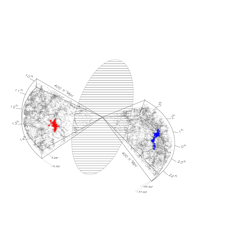
Figure 1.— The nearest, almost complete part of the 2dF GRS survey (up to 400 $h^{-1}$ Mpc). The two richest superclusters in this survey are shown. The disk showing the orientation of the galactic plane helps to allocate the 2dF survey in space; SCL 126 is located towards the Galactic North pole (left, red color), SCL 9 is at the right side of the figure (blue color).

The supercluster SCL126 is the most prominent supercluster defined by Abell clusters in the Northern 2dFGRS (SCL126 in the catalog of superclusters by E01, N152 in Paper I) in the direction of the Virgo constellation. This supercluster has also been called the Sloan Great Wall (Hoyle et al., 2002; Vogeley et al., 2004; Gott et al., 2005; Nichol et al., 2006). The presence of this supercluster affects the measurements of the correlation function (Croton et al., 2004), and of the genus and Minkowski functionals of the SDSS and 2dF redshift surveys (Park et al., 2005; Saar et al., 2007). The “meatball” shift in the measurements of the topology in the SDSS data is partly due to this supercluster (Gott et al., 2008).

The Sculptor supercluster, the most prominent supercluster in the Southern strip of the 2dFGRS, is among the three richest superclusters in E01; it contains 25 Abell clusters, six of these are also X-ray clusters. Zappacosta et al. (2005) found evidence about the presence of warm-hot diffuse gas there, which is associated with the inter-cluster galaxy distribution in this supercluster.

In a recent paper (Einasto et al., 2007d, hereafter RI) we studied the morphology of rich superclusters (their shape and internal structure), using Minkowski functionals and shapefinders. Our calculations in RI showed that the morphology of the richest superclusters from the 2dFGRS is different from each other: the supercluster SCL126 resembles a very rich filament (wall) with a high density core region, while the supercluster SCL9 can be described as a collection of spiders (a multi-spider), consisting of a large number of cores connected by relatively thin filaments.

The main aim of the present paper is to understand whether the differences in the overall morphology of these two rich superclusters under study are also reflected by their fine structure as determined by the distribution of galaxies of different luminosity, color and spectral type in core region and in outskirts of superclusters.

The first study to show that in a supercluster early and late type galaxies trace the structure of the supercluster in a different manner was performed by Giovanelli, Haynes & Chincarini (1986) who demonstrated that in the Perseus supercluster, elliptical galaxies are mainly located along the central body of the supercluster, while spiral galaxies are distributed in the outer regions of the supercluster. The presence of a large-scale segregation of galaxies of different type in nearby superclusters was shown also by Einasto & Einasto (1987). In Paper III we showed that rich superclusters have a larger fraction of red, non-star-forming galaxies than poor superclusters. Recently, galaxy populations have been studied in core regions of some very rich superclusters (Haines et al. (2006) – in the Shapley supercluster, Porter & Raychaudhury (2005) – in the Pisces-Cetus supercluster). These studies showed that rich clusters in the core regions of superclusters contain a large fraction of passive galaxies, while actively star forming galaxies are located between the clusters.

Thus studies of rich superclusters which contain a large variety of environments and possibly a variety of evolutionary phases give us a possibility to study the properties of cosmic structures and the properties of galaxies therein in a consistent way, helping us to understand the role of environment in galaxy evolution.

One method to quantify the structure of superclusters is to use the Minkowski functionals. This type of study has been called morphometry by Hikage et al. (2003). Minkowski functionals, genus and shapefinders, defined on the basis of Minkowski functionals have been used earlier to study the 3D topology of the large scale structure from 2dF and SDSS surveys (Saar et al., 2007; Hikage et al., 2003; Park et al., 2005; Gott et al., 2008; James, Lewis & Colless, 2007) and to characterize the morphology of superclusters (Sahni et al., 1998; Sheth et al., 2003; Shandarin et al., 2004; Basilakos et al., 2001; Kolokotronis, Basilakos & Plionis, 2002; Basilakos, 2003; Basilakos et al., 2006) from observations and simulations. These studies concern only the “outer” shapes of superclusters and do not treat their substructure. We expanded this approach in Paper RI by using the Minkowski functionals and shapefinders to analyze the full density distribution in superclusters, at all density levels.

The fourth Minkowski functional $V_{3}$ (the Euler characteristic) gives us the number of isolated clumps (or voids) in the region (Saar et al., 2007), meaning that we can use it to study the clumpiness of the galaxy distribution inside superclusters – the fine structure of superclusters. We calculate the fourth Minkowski functional $V_{3}$ for galaxies of different populations in superclusters for a range of threshold densities, starting with the lowest density used to determine superclusters, up to the peak density in the supercluster core. This analysis shows how the fourth Minkowski functional can be used in studies of the fine structure of superclusters as delineated by different galaxy populations. This study is of an exploratory nature since this is the first time when this method are used for studies of the fine structure of galaxy populations of individual superclusters. Employing Minkowski functionals, we can see in detail how the morphology of superclusters is traced by galaxies of different type.

In our analysis we use also the shapefinders calculated on the basis of the Minkowski functionals. In addition, we compare the galaxy content of groups of different richness in core regions and in outskirts of superclusters.

The paper is composed as follows. In Section 2 we describe the galaxy data, the supercluster catalogue and the data on the richest superclusters. In Sect. 3 we compare the overall galaxy content of the superclusters. In Sect. 4 we describe the use of the fourth Minkowski functional (the Euler characteristic) to study the fine structure of the superclusters as delineated by different galaxy populations. In Sect. 5 we study the galaxy content in the core regions and in the outskirts of the superclusters, and compare galaxy populations in groups of various richness. In the last sections (6 and 7) we discuss our results and give the conclusions. In the Appendix we give a definition of the Minkowski functionals and shapefinders, and describe different kernels used to calculate the density fields of superclusters.

2. Data

2.1. Rich supercluster data

We used the 2dFGRS final release (Colless et al., 2001, 2003), and the catalogue of superclusters of galaxies from the 2dF survey (Paper I), applying a redshift limit $z\leq 0.2$. When calculating (comoving) distances we used a flat cosmological model with the standard parameters, the matter density $\Omega_{m}=0.3$, and the dark energy density $\Omega_{\Lambda}=0.7$ (both in units of the critical cosmological density). Galaxies were included in the 2dF GRS, if their corrected apparent magnitude $b_{j}$ lied in the interval from $b_{1}=13.5$ to $b_{2}=19.45$. We used weighted luminosities to calculate the luminosity density field on a grid of the cell size of 1 $h^{-1}$ Mpc  smoothed with an Epanechnikov kernel of the radius 8 $h^{-1}$ Mpc; this density field was used to find superclusters of galaxies. We defined superclusters as connected non-percolating systems with densities above a certain threshold density; the actual threshold density used was 4.6 in units of the mean luminosity density. A detailed description of the supercluster finding algorithm can be found in Paper I.

In our analysis we also used the data about groups of galaxies from the 2dFGRS (Tago et al., 2006, hereafter T06). Groups in this catalogue were determined using the Friend-of-Friend (FoF) algorithm in which galaxies are linked together into a system if they have at least one neighbor at a distance less than the linking length. For details about the group finding algorithm and the analysis of the selection effects see T06. The catalogues of groups and isolated galaxies can be found at http://www.aai.ee/$\sim$maret/2dfgr.html, the catalogues of observed and model superclusters – at http://www.aai.ee/$\sim$maret/2dfscl.html. We present additional information about the morphology of the richest superclusters at http://www.aai.ee/$\sim$maret/richscl.html and http://www.aai.ee/$\sim$maret/rich2.html.

For the present analysis we select the richest superclusters from the catalogue of the 2dF superclusters. The data on these superclusters are given in Table LABEL:tab:1. In this Table we give the central coordinates, redshifts and distances of the superclusters, the numbers of galaxies, groups and Abell and X-ray clusters in the superclusters, the mean values of the luminosity density within superclusters and their total luminosities (from Paper II). In our morphological analysis we use volume-limited samples of galaxies from these superclusters. The luminosity limits for each supercluster sample are also given in Table LABEL:tab:1. We plot the sky distribution of galaxies, and Abell and X-ray clusters in Fig. 2; the location of these superclusters in space can be seen in Fig. 1.

Table 1Data on rich superclusters

ID	R.A.	Dec	Dist	$z$	$N_{gal}$	$M_{lim}$	$N_{vol}$	$N_{cl}$	$N_{gr}$	$N_{ACO}$	$N_{X}$	$\delta_{m}$	$L_{tot}$
	deg	deg	$h^{-1}$ Mpc
SCL126 (N152)	194.71	-1.74	251.2	0.085	3591	-19.25	1308	18	40,2	9	4	7.7	0.378E+14
SCL9 (N34)	9.85	-28.94	326.3	0.113	3175	-19.50	1176	24	26,9	12 (25)	2(6)	8.1	0.497E+14

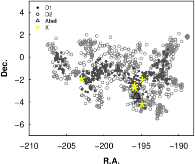
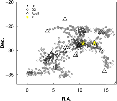
Figure 2.— The sky distribution of galaxies, and Abell and X-ray clusters in the superclusters SCL126 (left) and SCL9 (right). Filled gray circles: galaxies from the core region ($D1$, see sect. 5), empty gray circles: galaxies from the outskirt region ($D2$), triangles: Abell clusters, yellow stars: X-ray clusters.

The most prominent Abell supercluster in the Northern 2dF survey is the supercluster SCL126 that lies in the direction towards the Virgo constellation at a redshift $z=0.085$ (Paper I). This supercluster contains 7 Abell clusters: A1620, A1650, A1651, A1658, A1663, A1692, A1750. Of these clusters, A1650, A1651, A1663, and A1750 are X-ray clusters. The supercluster SCL126 is almost completely covered by the 2dF survey volume; only a small part of it lies outside the survey Einasto et al. (2003a). All Abell and X-ray clusters from this superclusters (9 and 6, correspondingly) are located in the region of the survey.

The richest supercluster in the Southern Sky is the Sculptor supercluster at a redshift $z=0.113$ (Paper I). This supercluster contains also several X-ray clusters, and the largest number of Abell clusters in our supercluster sample, 25. However, only 12 of them are located within the region covered by the 2dF supercluster S34. These are: A88, A122, A2751, A2759, A2778, A2780, A2794, A2798, A2801, and A2844, and two X- ray clusters, A2811 and A2829.

If we assume that the mean mass-to-light ratio is about 400 (in solar units), then we can estimate the masses of the richest superclusters of our sample, using the estimates of the total luminosity of the superclusters (Table LABEL:tab:1): $M_{SCL9}=2\times 10^{16}h^{-1}M_{\sun}$, $M_{SCL126}=1.5\times 10^{16}h^{-1}M_{\sun}$. These estimates are lower limits only, since the 2dF survey does not fully cover these superclusters. These masses are of the same order as the masses of other known very rich superclusters. For example, Proust et al. (2006) estimate that the total mass of the Shapley supercluster is at least $M_{tot}=5\times 10^{16}h^{-1}M_{\sun}$. Fleenor et al. (2005) give the same estimate for the total mass of the Horologium–Reticulum supercluster. Porter & Raychaudhury (2005) estimated that the total mass of the Pisces-Cetus supercluster is at least $M_{tot}=1.5\times 10^{16}h^{-1}M_{\sun}$. Thus our two superclusters have total masses similar to other rich superclusters.

2.2. Populations of galaxies used in the present analysis

We characterize galaxies by their luminosity, the spectral parameter $\eta$ and by the color index $col$ (Madgwick et al., 2002) and (Madgwick et al., 2003a; De Propris et al., 2003; Cole et al., 2005) as follows.

We divided galaxies into the populations of bright (B )and faint (F) galaxies, using an absolute magnitude limit $M_{bj}=-20.0$ (here and in the following, we give absolute magnitudes for $h=1,\quad H=100$ km/sec/Mpc; for any other value of $h$, the absolute magnitude $M=M_{h=1}+5\log h$). We chose this limit close to the characteristic luminosity $M^{*}$ of the Schechter luminosity function. The value of $M^{\star}$ is different for different galaxy populations Madgwick et al. (2003a); De Propris et al. (2003); Croton et al. (2005), having values from $-19.0$ to $-20.9$. We used an absolute magnitude limit $M_{bj}=-20.0$ as a compromise between the different values.

The absolute magnitude limits for the faintest galaxies in our superclusters (volume limited samples, $M_{lim}$) are given in Table LABEL:tab:1. Actually, our faint galaxy population is brighter than the faint galaxies analysed in several other superclusters, e.g. in the Shapley supercluster, (Mercurio et al., 2006; Haines et al., 2006), in the supercluster A2199 (a part of the Hercules supercluster SCL160 in E01 list) in Haines et al. (2006), and in the supercluster A901/902 (Gray et al., 2004).

We used the spectral parameter $\eta$ to divide galaxies into the populations of early (E) and late (S) type. We used for this purpose the spectral parameter limit $\eta=-1.4$: $\eta\leq-1.4$ for early type galaxies, and $\eta>-1.4$ for late type galaxies, and excluded galaxies with uncertain determination of $\eta$. More detailed morphological types were defined as follows: Type 1 (Kennicutt, 1992): $\eta<-1.4$; Type 2: $-1.4\leq\eta<1.1$; and Type 3: $1.1\leq\eta$.

Moreover, the spectral parameter $\eta$ is correlated with the equivalent width of the $H_{\alpha}$ emission line, thus being an indicator of the star formation rate in galaxies. Madgwick et al. (2003b) calls galaxies with $\eta>-1.4$ (late type galaxies) as ”generally star-forming”. Thus the spectral parameter gives us information on the types and star formation activity of galaxies.

Table 2 The superclusters SCL126 and SCL9: the number of galaxies in different galaxy populations, for the whole supercluster (volume limited samples), and for the core region ($D1$) and for the outskirts of the superclusters (D2)

(1)	(2)	(3)	(4)		(5)	(6)	(7)	(8)
	SCL126					SCL9
Region	All	$M_{bj}\leq-19.50$	$D1$	$D2$		All	$D1$	$D2$
Ngal	1308	932	488	820		1176	342	834
N$gr_{10}$	405	308	227	181		247	137	108
N$gr_{2}$	576	410	172	410		576	137	442
N$ig$	327	214	89	229		353	68	284
$E$	809	603	340	469		772	236	536
$S$	490	322	145	345		393	102	291
$r$	937	685	377	560		835	251	584
$b$	371	247	111	260		341	91	250
$B$	400	400	144	256		556	168	388
$F$	908	532	344	564		620	174	446

We used the rest-frame color index, $col=(B-R)_{0}$, to divide galaxies into the populations of red galaxies (r), $col\geq 1.07$, and blue galaxies (b), $col<1.07$ (Cole et al., 2005; Wild et al., 2005). Wild et al. (2005) suggest that red galaxies are mostly passive, and blue galaxies – actively star forming. However, since there exist also red galaxies showing signs of star formation (Wolf, Gray & Meisenheimer, 2005; Haines, Gargiulo & Merluzzi, 2008) we name our populations as red and blue.

In the next section we will analyse the relationship between the spectral parameters and color indexes of galaxies in our superclusters in more detail.

In our analysis we use following ratios: $E/S$ – the ratio of the numbers of early and late type galaxies, $r/b$ – the ratio of the numbers of red and blue galaxies, and $B/F$ – the ratio of the numbers of bright ($M_{bj}\leq-20.0$) and faint ($M_{bj}>-20.0$) galaxies.

3. Galaxy content of rich superclusters

First we study an overall galaxy content of the rich superclusters (see Table LABEL:tab:s1269d1d2ngal) . We plot the differential luminosity functions, and the distributions of the spectral parameter $\eta$ and the color index $col$ for galaxies from superclusters SCL126 and SCL9 in Fig. 3. For comparison we plot also the distribution of the spectral parameter $\eta$ and the color index $col$ for field galaxies, chosen from the same redshift interval as our two superclusters, and having the same absolute magnitude limit ($M_{bj}=-19.50$, see below). There are 1975 galaxies in the Northern field sample, $N(field)$, and 2927 in the Southern field sample, $S(field)$. The number of galaxies in field samples is rather small due to absolute magnitude limit used here, since, in general, galaxies in the field are fainter than in superclusters (Paper III). The comparison with field galaxies shows whether the possible differences between the distributions of spectral parameters and colors may be due to redshift differences between the two superclusters.

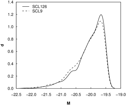
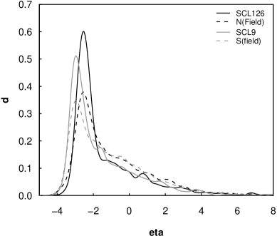
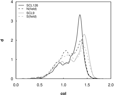
Figure 3.— The distribution of the absolute magnitude (left panel), the spectral parameter $\eta$ (middle panel) and the color index $col$ (right panel) of galaxies in the supercluster SCL126 (solid line), and in SCL9 (dashed line), both for the absolute magnitude limit $M_{bj}\leq-19.50$).

All the distributions (probability densities) shown in this paper have been obtained using the R environment (Ihaka & Gentleman, 1996), http://www.r-project.org (the ’stats’ package). This package does not provide the customary error limits; we discuss these limits in the appendix and show that they are small (about 4–5%).

In Table LABEL:tab:r2overall we give the ratios of the numbers of galaxies of different type in the superclusters; for SCL126 for two magnitude limits, the original (Table  LABEL:tab:1), and the SCL9 magnitude limit $M_{bj}=-19.50$, in order to compare these ratios with those calculated for the supercluster SCL9.

The Kolmogorov-Smirnov test, Fig. 3, and Table LABEL:tab:r2overall show differences in the overall galaxy content of the two richest 2dFGRS superclusters.

The Kolmogorov-Smirnov test shows that the probability that the distributions of luminosities of the two superclusters are drawn from the same parent sample is 0.135, having marginal statistical significance. The most important difference between the luminosities of the galaxies of two superclustes is that the brightest galaxies in SCL126 are brighter than those in SCL9. In Sect. 5 we show that there are also other differences in the distribution of the brightest galaxies in the two superclusters under study.

Table 3The galaxy content of the superclusters SCL126 and SCL9.

Sample	SCL126		SCL9
(1)	(2)	(3)	(4)
$M_{bj^{lim}}$	-19.25	-19.50	-19.50
Ngal	1308	932	1176
F$gr_{10}$	0.31	0.33	0.21
F$gr_{2}$	0.44	0.44	0.49
F$ig$	0.25	0.23	0.30
$E/S$	1.65	1.87	1.96
$r/b$	2.53	2.77	2.45
$B/F$	0.44	0.75	0.90

Next, Table LABEL:tab:r2overall shows that the ratio of the numbers of red and blue galaxies ($r/b$) is slightly larger in the supercluster SCL126, but the peak value of the color index of galaxies in this supercluster is smaller than in SCL9. The distributions of the spectral parameter $\eta$ and the color index $col$ both show large differences in the early type (red) galaxy content of the richest superclusters – in the supercluster SCL9, galaxies have larger color index values and smaller spectral parameter values than in supercluster SCL126.

According to the Kolmogorov-Smirnov test, the difference between the distributions of the spectral parameter $\eta$ and the color index $col$ of the two superclusters is highly significant. However, the comparison with the field galaxies of the same distance interval and absolute magnitude limit as the galaxies from superclusters, shows that the main reason for the differences of spectral parameters and colors is the difference in their distances (Fig. 3). This effect is difficult to quantify exactly, as the color distributions for supercluster and field galaxies differ in detail, but are close in the average. We illustrate their similarity by comparing in Table LABEL:tab:r2red the quartiles for the distributions of the spectral parameter $\eta$ and the color index $col$, for parameter intervals which correspond to early type and red galaxies ($\eta\leq-1.4$ and $col\geq 1.07$, correspondingly), for the absolute magnitude limit $M_{bj}=-19.50$. These quartiles are very similar for the supercluster and field galaxies.

Table 4The early type and red galaxy content of the superclusters SCL126 and SCL9.

SCL	$N{gal}$	lower quartile	median	upper quartile
(1)	(2)	(3)	(4)	(5)
$\eta<-1.4$
SCL126	603	-2.72	-2.49	-2.19
N(Field)	1053	-2.80	-2.47	-2.05
SCL9	772	-3.08	-2.78	-2.30
S(Field)	1583	-3.08	-2.71	-2.11
$col>1.07$
SCL126	685	1.23	1.32	1.37
N(Field)	1235	1.19	1.30	1.37
SCL9	835	1.27	1.39	1.47
S(Field)	1862	1.21	1.36	1.45

These differences, however, do not affect our calculations of the Minkowski functionals for individual superclusters. So there is no need to correct the colors and spectral parameters for this effect.

Next we present the color-magnitude diagrams for our two superclusters under study (Fig. 4). Interestingly, this figure shows that there is no correlation between the color and magnitude among the red galaxies in our superclusters. In this respect the color-magnitude diagrams for the superclusters SCL126 and SCL9 are different from those for some other superclusters, e.g., for the supercluster A901/902 (Gray et al., 2004) and for the core of the Shapley superclusters (Haines et al., 2006). The reasons for that are probably the use of total magnitudes in our study (see also Cross et al., 2001), in this case the color-magnitude relation is almost flat (Scodeggio, 2001), and the use of the data about relatively bright galaxies only. The studies by (Gray et al., 2004; Haines et al., 2006) include much fainter galaxies than those used in our study; for fainter galaxies the slope of the color-magnitude diagram is larger than for bright galaxies (see also Metcalfe, N., Godwin, J.G. & Peach, J.V.,, 1994) even when using total magnitudes, as mentioned by Scodeggio (2001). Thus Fig. 4 suggests that we can use galaxy colors for classification without further corrections.

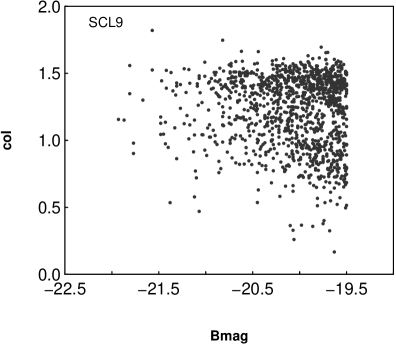
Figure 4.— The color-magnitude diagrams for the superclusters SCL126 (left panel) and SCL9 (right panel).

Finally, we take a closer look to the classification of galaxies by their spectral parameters and colors. For that we plot in Fig. 5 the joint distribution of the spectral parameter $\eta$ and the color index $col$ for the superclusters SCL126 and SCL9, in analogy to Fig. 2 in Wild et al. (2005). We see that most galaxies populate an area at the lower right quadrant, where the galaxies have spectra characteristic to early type galaxies (with no star formation) and have red colors. The upper left quadrant of this Figure is populated by late type, blue galaxies. But there are also galaxies, which have spectra characteristic to late type (”generally star forming”) galaxies, and in the same time have red colors. The number of these galaxies is small – 161 in the supercluster SCL126, and 114 in the supercluster SCL9. There are also galaxies with blue colors and spectra characteristic to early type galaxies (41 in SCL126 and 62 in SCL9). A detailed analysis of the properties of these galaxies is beyond the scope of the present paper, but below we discuss where these galaxies are located in superclusters and whether the differences between the populations of early type and red galaxies (and late type and blue galaxies) influence the calculation of the Minkowski functionals.

Figure 5.— The distribution of the spectral parameter $\eta$ and the color index $col$ of galaxies in the supercluster SCL126 (left panel), and in SCL9 (right panel). The solid lines separate early and late-type galaxies ($\eta=-1.4$), and red and blue galaxies ($col=1.07$).

4. Minkowski Functionals

4.1. Method

The supercluster geometry (morphology) is given by their outer (limiting) isodensity surface, and its enclosed volume. When increasing the density level over the outer threshold overdensity $\delta=4.6$ (sect. 2.1), the isodensity surfaces move into the central parts of the supercluster. The morphology and topology of the isodensity contours is (in the sense of global geometry) completely characterized by the four Minkowski functionals $V_{0}$–$V_{3}$.

For a given surface the four Minkowski functionals (from the first to the fourth) are proportional to: the enclosed volume $V$, the area of the surface $S$, the integrated mean curvature $C$, and the integrated Gaussian curvature (or Euler characteristic) $\chi$. The Euler characteristic describes the topology of the surface; at high densities it gives the number of isolated clumps (balls) in the region, at low densities – the number of cavities (voids) (see, e.g. Saar et al., 2007). This is the functional we shall use in this paper (see Appendix for details).

We calculate also the shapefinders $H_{1}$ (thickness), $H_{2}$ (width), and $H_{3}$ (length), which have dimensions of length, and dimensionless shapefinders $K_{1}$ (planarity) and $K_{2}$ (filamentarity) (see Appendix for definitions). In paper RI we showed that in the $K_{1}$-$K_{2}$ shapefinder plane the morphology of superclusters is described by a curve which is characteristic of multi-branching filaments; we call it a morphological signature.

In order to estimate the Minkowski functionals, we have to ensure that the mean density is constant throughout the volume we study. This is the main reason why we use volume limited samples of supercluster galaxies. This also means that we have to recalculate the (luminosity) density field; the field used to select superclusters was calculated on the basis of the full sample.

To obtain the density field for estimating the Minkowski functionals, we used a kernel estimator with a $B_{3}$ box spline as the smoothing kernel, with the total extent of 16 $h^{-1}$ Mpc (for a detailed description see Saar et al., 2007, and Paper RI). This kernel covers exactly the 16 $h^{-1}$ Mpc extent of the Epanechnikov kernel, used to obtain the original density field, but it is smoother and resolves better density field details (its effective width is about 8 $h^{-1}$ Mpc). The density field for both superclusters is shown in Fig. 6.

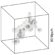
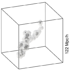
Figure 6.— The luminosity density distribution in the two superclusters. Left panel: SCL126, right panel: SCL9. The isosurfaces show the outer border of a supercluster and the density level for $m_{f}=0.7$. Dots show individual galaxies. Darker regions: core (D1), lighter regions - outskirts (D2).

As the argument labeling the isodensity surfaces, we chose the (excluded) mass fraction $m_{f}$ – the ratio of the mass in regions with density lower than the density at the surface, to the total mass of the supercluster. When this ratio runs from 0 to 1, the iso-surfaces move from the outer limiting boundary into the center of the supercluster, i.e. the fraction $m_{f}=0$ corresponds to the whole supercluster, and $m_{f}=1$ to its highest density peak. This is the convention adopted in all papers devoted to the morphology of the large-scale galaxy distribution.

At small mass fractions the isosurface includes the whole supercluster and the value of the 4th Minkowski functional $V_{3}=1$. As we move to higher mass fractions, the isosurface includes only the higher density parts of superclusters. Individual high density regions in a supercluster, which at low mass fractions are joined together into one system, begin to separate from each other, and the value of the fourth Minkowski functional ($V_{3}$) increases. At a certain density contrast (mass fraction) $V_{3}$ has a maximum, showing the largest number of isolated clumps in a given supercluster. At still higher density contrasts only the high density peaks contribute to the supercluster and the value of $V_{3}$ decreases again.

In Paper RI we showed that according to Minkowski functionals, the supercluster SCL126 resembles a multibranching filament with a high density core at a mass fraction $m_{f}\approx 0.95$. The maximum value of the fourth Minkowski functional, $V_{3}$, in this supercluster is 9. The main body of this filament is seen in Fig. 2 (region $D1$, see below for definition).

The supercluster SCL9 can be described as a multispider rather than a rich filament, i.e. this supercluster consists of a large number of relatively isolated clumps or cores connected by relatively thin filaments, in which the density of galaxies is too low to contribute to the higher density parts of this supercluster. The maximum value of the fourth Minkowski functional, $V_{3}$, in this supercluster is 15, i.e. this supercluster is more clumpy than the supercluster SCL126. The main cores of this supercluster are seen in Fig. 2 as region $D1$.

Now we shall find the Minkowski functional $V_{3}$ and morphological signature $K_{1}$-$K_{2}$ for rich superclusters separately for galaxies from different populations, as marked by their luminosity, the spectral parameter $\eta$ and the color index $col$ (Figs. 7 and  8). To understand better the morphological signature we show the shapefinders $H_{1}$, $H_{2}$ and $H_{3}$ (Fig. 9). To not to overcrowd the paper with Figures we show the shapefinders for the supercluster SCL126 for bright and faint galaxies only.

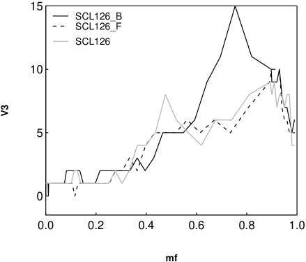
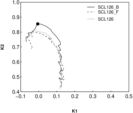
Figure 7.— The supercluster SCL126. Upper panels: the Minkowski functional $V_{3}$ (the Euler characteristic) vs the mass fraction $m_{f}$ for bright (B, $M\leq-20.0$) and faint (F, $M>-20.0$) galaxies (left panel), for early and late type galaxies (middle panel) and for red and blue galaxies (right panel). Lower panels: the morphological signatures $K_{1}$ (planarity) – $K_{2}$ (filamentarity) for the same populations. Triangles show the values of $K_{1},~{}K_{2}$, where the mass fraction $m_{f}=0.0$ (the whole supercluster), and filled circles – the values of $K_{1},~{}K_{2}$, which correspond to the $m_{f}=0.7$. In the left panels we also plot the $V_{3}$ and $K_{1},~{}K_{2}$ curves for the whole supercluster (light grey line).

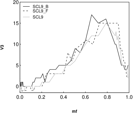
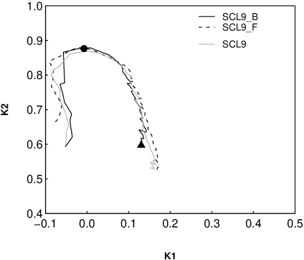
Figure 8.— The supercluster SCL9. Upper panels: the Minkowski functional $V_{3}$ (the Euler characteristic) vs the mass fraction $m_{f}$ for bright (B, $M\leq-20.0$) and faint (F, $M>-20.0$) galaxies (left panel), for early and late type galaxies (middle panel) and for red and blue galaxies (right panel). Lower panels: the morphological signatures $K_{1}$ (planarity) - $K_{2}$ (filamentarity) for the same populations. Symbols as in Fig. 7.

Figure 9.— From left to right: the shapefinders $H_{1}$ (thickness), $H_{2}$ (width), and $H_{3}$ (length) (in $h^{-1}$ Mpc) for the supercluster SCL126, for bright (B, $M\leq-20.0$) and faint (F, $M>-20.0$) galaxies.

4.2. SCL126

Fig. 7 (upper left panel) shows the $V_{3}$ curves for bright and faint galaxies in the supercluster SCL126. At small values of the mass fraction $m_{f}$ the values of $V_{3}$ are small. At a mass fraction $m_{f}\approx 0.4$ the values of $V_{3}$ of both bright and faint galaxies increase rapidly which shows that at this density level the supercluster is splitted into several clumps. For bright galaxies the $V_{3}$ curve has some small plateaus at $m_{f}\approx 0.6$ and $m_{f}\approx 0.7$, this curve reaches maximum value of about 15 at mass fraction $m_{f}\approx 0.9$.

For faint galaxies the value of $V_{3}$ increases at mass fraction $m_{f}\approx 0.4$. In the whole mass fraction interval the values of $V_{3}$ for faint galaxies are smaller than those for bright galaxies, about 5. This indicates that the overall distribution of bright galaxies is clumpy, while the distribution of faint galaxies is more homogeneous. The peaks of $V_{3}$ values at very high mass fractions where the maximum value of $V_{3}$ for faint galaxies is 10, are due to high - density cores in this supercluster. The $V_{3}$ curve for the full supercluster is very similar to that of $V_{3}$ curve for faint galaxies showing faint galaxies trace the structure of the supercluster rather well.

Fig. 7 (lower left panel) shows the shapefinders $K_{1}$ (planarity) and $K_{2}$ (filamentarity) for bright and faint galaxies. They are calculated on the basis of shapefinders $H_{1}$-$H_{3}$ (Fig. 9). Of these, the shapefinder $H_{1}$ is the smallest and characterizes the thickness of superclusters. The shapefinder $H_{2}$ is an analogy of the width of a supercluster, but it contains information about both the area and curvature of an isodensity surface. The shapefinder $H_{3}$ is the largest and describes the length of the superclusters. This is not the real length of the supercluster, but a measure of the integrated curvature of the surface.

Fig. 9 shows that at all mass fractions, the thickness $H_{1}$ and the width $H_{2}$ of the supercluster as determined using data about bright galaxies are smaller than those calculated using data about faint galaxies. Thus, at all density levels the distribution of bright galaxies is more compact than the distribution of faint galaxies (which is also less clumpy). However, the shapefinder $H_{3}$ which is calculated as $H_{3}=C/4\pi$ (the integrated mean curvature C) reflects the clumpiness of a population, and since the distribution of bright galaxies is much more clumpy (according to $V_{3}$), the value of $H_{3}$ for bright galaxies is larger than this value for faint galaxies (Fig. 9, right panel). This makes also the filamentarity $K_{2}$ for bright galaxies to be larger than the filamentarity of faint galaxies. As a result, in the morphological signature (Fig. 7, lower left panel) the values of $K_{2}$ for bright galaxies are larger. The morphological signature of faint galaxies is similar to that of the whole supercluster, this is another indication that faint galaxies trace the structure of the supercluster well.

In this Figure we marked the value of $K_{1}$ and $K_{2}$ at the mass fraction $m_{f}\approx 0.7$. Interestingly, we see that at this mass fraction (density level) the characteristic morphology of supercluster changes, as seen from the change of the morphological signature.

The values of the fourth Minkowski functional, $V_{3}$, for galaxies of different type (Fig. 7, upper middle panel, cassified by the spectral parameter $\eta$) show that the clumpiness of early type galaxies starts to increase at low values of the mass fraction, $m_{f}\approx 0.2-0.3$. At the mass fraction value $0.5$ the value of $V_{3}$ has a small peak followed by a minimum; at the mass fraction $m_{f}\approx 0.7$ the value of $V_{3}$ increases again, and has a peak value about 10 at the mass fraction of about 0.9.

The distribution of late-type galaxies in this supercluster is much less clumpy, as show the values of $V_{3}$. The number of isolated clumps of these galaxies grows only at rather high mass fraction values, $m_{f}>0.6$ ($V_{3}=6$), and has a peak at $m_{f}\approx 0.9$ (here $V_{3}=12$). The largest differences in the clumpiness of the spatial distribution of galaxies of different type are, according to the fourth Minkowski functional, at mass fractions $m_{f}<0.6$, which describe the outer (lower density) region of the supercluster.

Fig. 7 (lower middle panel) shows the morphological signature for galaxies of different type. The value of $K_{2}$ (filamentarity) that contains information both about the spatial extent and clumpiness of the data, is larger for late-type galaxies. In this figure an important feature is that, again, at the mass fraction (density level) $m_{f}\approx 0.7$ the characteristic morphology of supercluster changes.

The curves of the fourth Minkowski functional for red galaxies are rather similar to those of early type galaxies (Fig. 7, upper right panel, the color index $col$). Here we again see an increase of the values of $V_{3}$ at the mass fractions $m_{f}\approx 0.4$ and $m_{f}\approx 0.6$, and a maximum at $m_{f}\approx 0.9$ ($V_{3}=10$).

This panel shows that blue galaxies form a few isolated clumps already at relatively low mass fraction values, but those clumps have low density, and at higher mass fractions some of them do not contribute to the supercluster any more; the value of $V_{3}$ decreases (being smaller than 6) and then increases again at mass fractions $m_{f}\approx 0.6-0.7$. At this mass fraction the clumpiness of the blue galaxy distribution becomes comparable to that of red galaxies. At very high values of the mass fraction, $m_{f}>0.9$, blue galaxy clumps are not seen, and the value of $V_{3}$ decreases rapidly. The value of $V_{3}$ for red galaxies is larger than for blue galaxies at almost all density levels (mass fraction values).

At the mass fraction $m_{f}\approx 0.7$ (Fig. 7, lower right panel) the characteristic morphology of the supercluster, as described by red and blue galaxies, changes.

Thus Fig. 7 shows that the differences in clumpiness between galaxies of different type and color (and star formation rate) in the supercluster SCL126 are the largest, according to the fourth Minkowski functional, at mass fractions $m_{f}<0.7$, which describe the outer (lower density) regions of the supercluster. In outer parts of this supercluster, the distribution of late type and blue galaxies is much less clumpy (more homogeneous) that the distribution of early type, red galaxies.

The fourth Minkowski functional $V_{3}$ for early type galaxies (Fig. 7, middle panel) has a small peak at mass fractions of about $0.4<m_{f}<0.6$ where the value of $V_{3}=10$. This indicates that at this intermediate density level early type galaxies form some isolated clumps which at still higher density level (mass fraction) do not contribute to supercluster any more, and the value of $V_{3}$ decreases again. At the same mass fractions $V_{3}$ for red galaxies (right panel) has a value $V_{3}=7$ with no peak. Therefore, these additional isolated clumps are due to early type blue galaxies. The galaxies that are classified as late type but have red colors are located in intermediate density filaments which connect clumps of early type galaxies to the main body of the supercluster.

4.3. SCL9

Next let us study the values of $V_{3}$ for galaxies of different populations in the supercluster SCL9 (Fig. 8, upper right panel). Here we see that the $V_{3}(m_{f})$ curve is rather different from that for SCL126: at small mass fractions, the values of $V_{3}$ for bright and faint galaxies (left panel) are small, but at a mass fraction value of about 0.4, the values of $V_{3}$ increase. This increase is more rapid for bright galaxies than for faint galaxies. The values of $V_{3}$ for bright galaxies reach a maximum at a mass fraction $m_{f}\approx 0.7$, and the maximum values of $V_{3}$ are larger than in the supercluster SCL126, about 18. For faint galaxies the $V_{3}$ curve reaches the maximum value, 15, at the mass fraction $m_{f}\approx 0.7$. The clumpiness of both the bright and faint galaxy distribution in the supercluster SCL9 is larger than that in the supercluster SCL126. Also in this supercluster the $V_{3}$ curve for the full supercluster is very similar to that of the $V_{3}$ curve for faint galaxies showing that faint galaxies trace the structure of the supercluster well.

In the middle right panel of Fig. 8 ($V_{3}$ for early and late type galaxies, defined by the spectral parameter $\eta$) we see a continuous increase of the number of isolated clumps as delineated by galaxies of different type. Interestingly, up to mass fractions of about $m_{f}=0.7$ the $V_{3}$ curves for galaxies of different type almost coincide ($V_{3}=12)$, which is opposite to what we saw in SCL126. Then the number of clumps in the distribution for late type galaxies increases rapidly and reaches the maximum value, 20, at mass fractions between 0.7 and 0.8. The distribution of late type galaxies in the core region of the supercluster SCL9 is even more clumpy than the distribution of early type galaxies.

The curves for $V_{3}$ for red and blue galaxies (divided using the color index $col$, upper left panel of Fig. 8) are quite similar to those we saw above. Up to the mass fractions $m_{f}\approx 0.7$ (the outer regions of the supercluster) the $V_{3}$ curves for galaxies of different color almost coincide. In the core region of the supercluster the distribution of blue galaxies is very clumpy, the maximum number of clumps is 17, while the maximum number of isolated clumps in the distribution of red galaxies is 12. Larger values of $V_{3}$ for blue galaxies suggest again that in this supercluster, blue galaxies are located in numerous clumps, while the distribution of red galaxies is smoother.

This figure shows that at intermediate mass fractions, $0.4<m_{f}<0.6$, the values of $V_{3}$ for blue galaxies show a small peak not seen in the $V_{3}$ curve for the late type galaxies. This peak is generated by those galaxies that have blue colors, but spectra characteristic to early type galaxies. This is consistent with the overall large clumpiness of blue galaxies in this supercluster.

In Fig. 8 (lower panels) we plot the morphological signature for galaxies of different populations in SCL9. These figures show that also in this supercluster the filamentarity of bright galaxies is larger than the filamentarity of faint galaxies. The morphological signature of faint galaxies is similar to that of the whole supercluster. The filamentarity $K_{2}$ for late type, blue galaxies is larger than that for early type (and red) galaxies due to their larger clumpiness. However, we see in these figures again that at the mass fraction $m_{f}\approx 0.7$ the morphology of the supercluster changes.

4.4. Summary

The differences in the distribution of galaxies from different populations in the superclusters SCL126 and SCL9 are related to different overall morphology of these superclusters. In particular, in the supercluster SCL126 at mass fractions $m_{f}<0.7$ the differences in the fine structure formed by galaxies of different populations are large: here the maximum values of $V_{3}$ are, correspondingly, 8 for red galaxies and 5 for blue galaxies, showing that the distribution of blue, late type galaxies is more homogeneous than the distribution of red, early type galaxies. At mass fractions $m_{f}>0.7$ the clumpiness of the distribution of galaxies of different type and color in the supercluster SCL126 is similar. In the contrary, in the supercluster SCL 9 the clumpiness of galaxy populations of different type and color is quite similar in the outskirts of the supercluster (e.g., the values of $V_{3}$ are the same, 7–8 both for the early and late type galaxies). At mass fractions $m_{f}>0.7$ in this supercluster, the clumpiness of the late type, blue galaxy population is larger (the maximum value of $V_{3}$ is 17) than the clumpiness of the early type, red galaxy population (for those galaxies the maximum value is $V_{3}=12$). Overall, the clumpiness of all galaxy populations in the supercluster SCL126 is smaller than the clumpiness of galaxy populations in SCL9.

This shows that in superclusters under study there exists a region of mass fractions $m_{f}\approx 0.7$, where we can observe in the behaviour of both the fourth Minkowski functionals for galaxies of different type and of the morphological signature a crossover from low- density morphology to high-density morphology. Based on that, we choose the mass fraction $m_{f}=0.7$ to delimit the supercluster cores. In the following analysis we use this density level as separating the high density core regions of superclusters ($D1$) from their outer regions with lower densities (outskirts, $D2$), see Fig. 2.

The density level $m_{f}=0.7$ approximately corresponds to region where the luminosity density contrast $\delta=10$ (Papers I and III). In Paper III we showed that high density cores with $\delta>10.0$ are characteristic to rich superclusters. Typical densities in poor superclusters are lower, $\delta<10.0$, comparable to densities in the outskirts of rich superclusters.

In both superclusters, about 3/4 of late type galaxies with red colors, as well as those galaxies showing blue colors and early type spectra, are located at intermediate densities in the outskirt regions. Fig. 7 and Fig. 8 show that although due to these galaxies the values of the fourth Minkowski functional $V_{3}(m_{f})$ for galaxies of different type and color differ in some details, the overall shapes of $V_{3}(m_{f})$ curves show no systematic differences.

Fig. 2 shows the main body of the supercluster SCL126 as a rich filament (region $D1$; paper RI). The main core of the supercluster at R.A. about 195 deg contains four Abell clusters (three of them are also X- ray sources). This region has a diameter of about 10 $h^{-1}$ Mpc (Einasto et al., 2003a). The X-ray cluster at R.A. about 203 deg is Abell 1750, a merging binary cluster (Donelly et al., 2001; Belsole et al., 2004).

In the supercluster SCL9 the regions of highest density form several separate concentrations of galaxies (a ”multispider”, Fig. 2 and RI). One of them, the main center of SCL9, contains 5 Abell clusters and one X-ray cluster. There are Abell clusters also in outskirts of this supercluster. In this supercluster the total number of Abell clusters is larger than in the supercluster SCL126, but they do not form such a high concentration of Abell and X-ray clusters that is observed in the core region of SCL126.

In the following section we study the distribution of galaxies from various populations in the core region and in outskirts of superclusters, using additionally the information about the group membership for galaxies from different populations.

We mention here that the values of $V_{3}(m_{f})$ reflect the distribution of galaxies at scales determined by the width of our smoothing kernel, B3, and this corresponds to larger scales than the typical scale at which the relation between galaxy type and local density applies, i.e. our results do not reflect directly features in galaxy distribution with characteristic scale less than about 1 - 2 $h^{-1}$ Mpc.

Thus the differences in clumpiness of galaxies of different type at high mass fractions (in supercluster cores) does not contradict to the presence of the luminosity - density relation at small scales. At the same time, the brightest galaxies of both early and late type galaxies are located in high density regions and this is seen also in $V_{3}(m_{f})$ curves at high mass fraction (Hamilton, 1988; Einasto, 1991; Park et al., 2007).

5. Substructure of superclusters in core region and in outskirts. Rich and poor groups

5.1. Core and outskirts

Groups of galaxies are additional tracers of substructure in superclusters. The group richness is a local density indicator, if we compare the properties of galaxies in various local environments (Paper III). We divide groups by their richness as follows: rich ($N_{gal}\geq 10$) groups and clusters (we denote this sample as $Gr_{10}$) and poor groups ($N_{gal}<10$, $Gr_{2}$). In Table LABEL:tab:r2overall we give the fractions of galaxies in these groups for the whole superclusters.

Let us study the galaxy content of groups in the cores and in the outskirts of our superclusters. We plot the differential luminosity functions and the distributions of the spectral parameter $\eta$ and the color index $col$ for galaxies in groups of different richness in Figs. 10–11, for the core regions and outskirts of the superclusters SCL126 and SCL9, respectively. In Table LABEL:tab:s1269d1d2 we present the ratios of the numbers of bright and faint galaxies $B/F$ in superclusters, and the ratios of early and late type galaxies $E/S$, as classified by the spectral parameter $\eta$. We also calculate the ratio of the numbers of red and blue galaxies, $r/b$, classified by the color index $col$. We give here the statistical significance of the differences between the galaxy content in core regions and in outskirts in these two superclusters according to the Kolmogorov-Smirnov test.

Table 5The superclusters SCL126 and SCL9: the galaxy content in the core region D1 and in the outskirts (region D2), in rich and poor groups, and of those galaxies which do not belong to groups.

(1)	(2)	(3)	(4)	(5)	(6)	(7)	(8)	(9)
		SCL126			SCL9
Region	$D1$	$D2$	Kolmogorov-Smirnov		$D1$	$D2$	Kolmogorov-Smirnov
			test results				test results
			$D$	$P$			$D$	$P$
Ngal	488	820			342	834
F$gr_{10}$	0.46	0.22			0.40	0.13
F$gr_{2}$	0.35	0.50			0.40	0.53
F$ig$	0.18	0.28			0.20	0.34
$E/S$
$All$	2.34	1.36	0.13	5.39e-05	2.31	1.84	0.10	0.02
$Gr_{10}$	4.35	2.81	0.13	0.088	4.07	3.20	0.17	0.05
$Gr_{2}$	1.68	1.40	0.08	0.452	2.05	2.07	0.06	0.77
$IG$	1.26	0.78	0.19	0.240	1.16	1.33	0.12	0.38
$r/b$
$All$	3.40	2.15	0.11	0.001	2.76	2.34	0.08	0.07
$Gr_{10}$	7.37	4.01	0.11	0.16	5.00	3.77	0.13	0.29
$Gr_{2}$	2.46	2.36	0.06	0.79	2.34	2.61	0.06	0.84
$IG$	1.62	1.26	0.12	0.28	1.48	1.71	0.11	0.48
$B/F$
$All$	0.42	0.45	0.07	0.165	0.96	0.87	0.04	0.72
$Gr_{10}$	0.47	0.59	0.09	0.34	1.00	0.91	0.10	0.61
$Gr_{2}$	0.44	0.46	0.14	0.01	1.00	0.95	0.05	0.97
$IG$	0.27	0.35	0.09	0.66	0.81	0.75	0.06	0.99

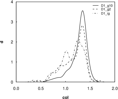
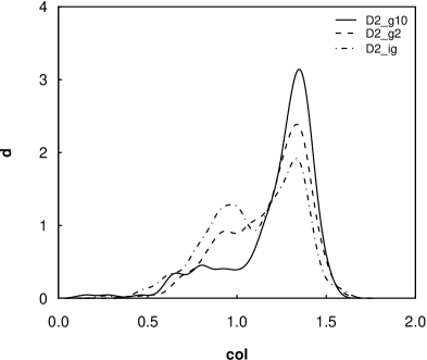
Figure 10.— The distributions of the absolute magnitude (upper panels), the spectral parameter $\eta$ (middle panels) and the color index $col$ (lower panels) of galaxies in groups of various richness in the supercluster SCL126. Left panels: the core (region $D1$), right panels: the outskirts (region $D2$). The populations are: $g10$ – rich groups ($N_{gal}\geq 10$), $g2$ – poor groups ($N_{gal}<10$), and $ig$ – isolated galaxies (those galaxies which do not belong to any group). The Kolmogorov-Smirnov test results for the difference of the distributions are in Table LABEL:tab:s1269d1d2.

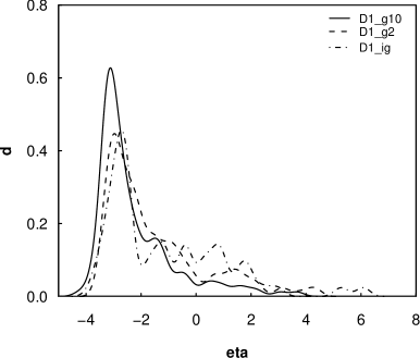
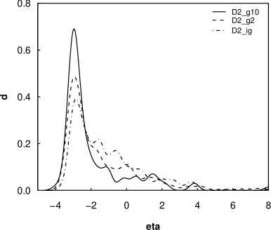
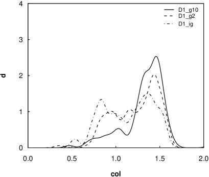
Figure 11.— The distributions of the absolute magnitude (upper panels), the spectral parameter $\eta$ (middle panels) and the color index $col$ (lower panels) of galaxies in groups of various richness in the supercluster SCL9. Left panels: the core (region $D1$), right panels: the outskirts (region $D2$). The populations are: $g10$ – rich groups ($N_{gal}\geq 10$), $g2$ – poor groups ($N_{gal}<10$), and $ig$ – isolated galaxies (those galaxies which do not belong to any group).The Kolmogorov-Smirnov test results for the difference of the distributions are in Table LABEL:tab:s1269d1d2.

5.2. SCL126

Fig. 10 (upper row) shows the luminosities of galaxies in groups of different richness in the supercluster SCL126. This figure shows that the brightest galaxies reside in rich groups ($N_{gal}\geq 10$), both in the core region and in the outskirts of the supercluster. Luminosities of galaxies in poor groups are fainter, and galaxies which do not belong to groups are the faintest, although in the core region of the supercluster there are also some rather bright galaxies among them.

According to the spectral parameter $\eta$ (Fig. 10, middle row), rich groups in the core region of the supercluster SCL126 are populated mainly with early type, quiescent galaxies (type 1 galaxies, $\eta<-1.4$). The fraction of late type galaxies in them is very small. The fraction of late type galaxies increases, as we move to poor groups. In the core region of the supercluster the fraction of late type galaxies is largest among those galaxies which do not belong to groups.

In the outskirts region, $D2$, rich groups are still mainly populated with early type galaxies, but the fraction of late type galaxies in them is larger ($E/S=2.81$) than in rich groups in the core region, where $E/S=4.35$. The fraction of late type galaxies in poor groups is larger; the fraction of these galaxies is the largest among those galaxies which do not belong to any group. In the supercluster outskirts, the fraction of late type galaxies among those galaxies which do not belong to groups, is larger than among this population in the supercluster core.

Table LABEL:tab:s1269d1d2 shows that according to the Kolmogorov-Smirnov test, the differences between the distributions of the spectral parameter $\eta$ for galaxies in the core region and in the outskirts have very high statistical significance. The differences in the galaxy content of groups, and of those galaxies which do not belong to groups from the core region $D1$ and in the outskirts $D2$ are smaller, and their statistical significance is marginal.

The distribution of the color index $col$ for galaxies in the supercluster SCL126 (Fig. 10, lower row) shows that members of rich groups from the core region of the supercluster are mainly red galaxies, $col>1.07$. The fraction of blue galaxies is larger in poor groups, and this fraction is the largest among those galaxies which do not belong to groups. In the outskirts region, even in rich groups there is a larger fraction of galaxies having $col<1.07$, in comparison with the core region. Mostly, blue galaxies can be found among those galaxies which do not belong to groups. The differences between the galaxy content of poor groups from the core region and the outskirts are smaller.

The statistical significances of these differences are given in Table LABEL:tab:s1269d1d2. This table shows that according to the Kolmogorov-Smirnov test, the differences between the distributions of the color index $col$ for galaxies in the core region and in the outskirts have very high statistical significance. Among other populations, the statistical significance of differences is marginal.

In other words, galaxies of different type in the supercluster SCL126 are segregated: red galaxies are preferentially located in rich groups, and blue galaxies in poor groups and among those galaxies not in any group. This is in a good accordance with the results about the fine structure obtained with the fourth Minkowski functional $V_{3}$ where we saw that red galaxies in the supercluster SCL126 are more clumpy, while blue, galaxies formed a less clumpy populations around them.

5.3. SCL9

The distribution of galaxies from different populations in the supercluster SCL9 is shown in Fig. 11 and Table LABEL:tab:s1269d1d2.

We see, in accordance with the data about SCL126, that galaxies in rich groups are, in average, brighter than galaxies in poor groups; galaxies which do not belong to groups are fainter than group galaxies. The largest difference between the distribution of galaxies by luminosity in the superclusters SCL126 and SCL9 is that in the supercluster SCL9 the luminosities of the brightest galaxies in rich and poor groups are of the same order.

In the supercluster SCL9 the fraction of early type, red galaxies is again the largest in rich groups and the smallest among those galaxies which do not belong to groups. However, in this supercluster rich groups contain also a large fraction of late type, blue galaxies, especially in the outskirts of the supercluster. The fraction of blue galaxies in poor groups of the core region is also relatively large. Thus, in contrast to the supercluster SCL126, in the supercluster SCL9 early and late type, and red and blue galaxies reside together in groups of different richness. This is the same structure that was shown by the fourth Minkowski functional - blue galaxies form numerous small clumps.

Table LABEL:tab:s1269d1d2 shows that according to the Kolmogorov-Smirnov test, the differences between the distributions of the spectral parameter $\eta$ for galaxies in the core region and in the outskirts in the supercluster SCL9 are statistically significant. The differences between the distributions of the color index $col$ for galaxies in the core region and in the outskirts have a lower statistical significance. The differences between the distributions of luminosities for galaxies in the core region and in the outskirts have a marginal statistical significance only.

5.4. Summary

The Table LABEL:tab:s1269d1d2 shows that the overall galaxy content of supercluster cores and outskirts is different. In the core regions, the fraction of galaxies located in rich groups is about 0.45, while the fraction of galaxies in rich groups in the outskirt region is about 0.20. The fraction of those galaxies which do not belong to any group in the core region is smaller than in the outskirt region.

The core regions contain about 1.5 times more of early type, red galaxies than the outskirts. The statistical significance of these differences is high. What we see here is an evidence for a large scale morphology-density relation in superclusters – high density cores of superclusters contain relatively more early type, red galaxies than the lower density outer regions.

Interestingly, the galaxy content of groups in the superclusters SCL126 and SCL9 is not similar. In the supercluster SCL126 galaxies of different type are segregated: red galaxies are preferentially located in rich groups, and blue galaxies in poor groups and among those galaxies not in any group. In the supercluster SCL9 early and late type, and red and blue galaxies reside together in groups of different richness.

This is in a good accordance with the results about the fine structure of superclusters delineated by galaxies from different populations obtained using the fourth Minkowski functional $V_{3}$.

In both superclusters, those galaxies classified as late type but having red colors, and blue galaxies with early type spectra are mostly located in poor groups or they do not belong to any group; only about 10% of them are located in rich groups.

Another important difference between these superclusters is that in the supercluster SCL126 the brightest galaxies reside in rich groups while in the supercluster SCL9 the luminosity of the brightest galaxies in rich and poor groups is the same.

In summary, the high-density cores of the superclusters contain relatively more early-type, quiescent, red galaxies than the lower-density regions, where there are more blue, star-forming galaxies. In the core regions the fraction of galaxies in rich groups is larger than this fraction in the outskirts. This shows that both the local (group/cluster) and the global (supercluster) environments are important in influencing types, colors and star formation rates of galaxies.

Earlier studies ((Davis & Geller, 1976; Dressler, 1980; Einasto & Einasto, 1987; Phillipps et al., 1998; Norberg et al., 2001, 2002; Zehavi et al., 2002; Goto et al., 2003; Hogg et al., 2003, 2004; Balogh et al., 2004; De Propris et al., 2003, 2004; Madgwick et al., 2003b; Croton et al., 2005; Blanton et al., 2004, 2006, among others) have shown the difference between the galaxy populations in clusters and in the field. Our results show that this difference exists also between the core regions and the outer regions of rich superclusters (see also Paper III).

6. Discussion

6.1. Selection effects

Both rich superclusters, SCl126 and SCL9, are not fully covered by the survey volume of the 2dFGRS. However, in the case of the supercluster SCL126 only its small, outer part remains outside the survey (see references in sect. 2). All rich clusters in this supercluster are included. Thus, most probably, including the full supercluster may add a relatively small number of mainly blue galaxies to this supercluster; this would not change our results about the galaxy content and fine structure in the supercluster core region and about rich groups in the outskirts of the supercluster.

With the supercluster SCL9, the situation is more complicated. The part which remains outside contains about half of the Abell clusters in this supercluster (sect. 2). Therefore, including them would increase the maximum values of the fourth Minkowski functional, $V_{3}$, since this characteristic counts the number of isolated clumps in an object under study. Thus, the differences between the values of $V_{3}$ for superclusters SCL126 and SCL9 would even increase. Even in the present analysis we saw that the values of $V_{3}$ for blue galaxies for SCL9 are larger than those values for SCL126. Thus, even if in the remaining part of the supercluster blue galaxies were distributed homogeneously such as not to increase the present values of $V_{3}$ (not a very probable case!) the differences between the $V_{3}$ values for galaxies of different type would not disappear.

Similarly, the differences in the galaxy content of groups from the core region and the outskirts would not disappear unless the distribution and clumpiness of galaxies in the (excluded) part of the supercluster SCL9 were completely different from what we see in its 2dFGRS part. Probably we should not expect to see large variations in the galaxy content of different parts of one supercluster. Moreover, in paper III we showed that the scatter in galaxy populations of superclusters is small.

For a more detailed study we plan to analyse a larger number of rich superclusters. For that, we started to generate supercluster catalogues using the SDSS data. In particular, the region of the supercluster SCL126 is covered by both surveys, therefore giving us a good chance to compare the properties of this supercluster, enclosed by both data sets.

6.2. Comparison with other very rich superclusters

The richest relatively nearby supercluster is the Shapley Supercluster (Proust et al., 2006, and references therein) (Bardelli et al., 2000; Quintana et al., 2000). The main core of this supercluster contains at least two Abell clusters and two X-ray groups. Haines et al. (2006) studied the galaxy populations in the core region of this supercluster using data about galaxies with fainter absolute magnitude limit than used in our study, thus we can compare their results with ours qualitatively only. They demonstrated that the colors of galaxies in the core region of the Shapley supercluster depend on their environment, with redder galaxies being located in clusters. They also found a large amount of faint blue galaxies between the clusters. We found the same trends with colors, especially in the core region of the supercluster SCL126. Haines et al. found also that in the core of the Shapley supercluster there where the fraction of blue galaxies is the lowest, the X-ray emission is the strongest. As seen above, we also find that in rich groups, which have X-ray sources, the fraction of blue galaxies is very small (the core region of SCL126).

Porter and Raychaudhury studied recently another rich supercluster partly covered by the 2dF surevy – the Pisces-Cetus supercluster (SCL10 in E01) (Porter & Raychaudhury, 2005, 2007). They used data about Abell clusters, galaxy groups (by Eke et al., 2004) and galaxies in this supercluster. Porter and Raychaudhury used the spectral parameter $\eta$ to determine the star formation rates for galaxies in groups in this supercluster. They concluded that galaxies in rich clusters have lower star formation rates than galaxies in poor groups in agreement with our results. Porter and Raychaudhury also demonstrated that in the filament between the clusters in this supercluster the fraction of star forming galaxies is higher at larger distance from clusters than close to clusters.

Gray et al. (2004) studied the environment of galaxies of different colors in the supercluster A901/902. They divided galaxies into red (quiescent) and blue (star-forming) populations, using $(U-V)$ colors of galaxies brighter than $M_{v}\approx-14$. Gray et al. (2004) obtained strong evidence that the highest density regions in clusters are populated mostly with red, quiescent galaxies, while blue, star-forming galaxies dominate in outer/lower density regions of clusters. Our samples do not contain very faint galaxies; for brighter galaxies, we find qualitatively the same trends in our superclusters.

Wolf, Gray & Meisenheimer (2005) showed that in the supercluster A901/902 there exists a population of dusty red galaxies which show red colors and also signatures of star formation. In this supercluster these galaxies are located at intermediate densities. This agrees well with our finding about galaxies with mixed classification (galaxies with red colors and spectra typical to late type galaxies): these galaxies populate mostly intermediate density regions of superclusters, being members of poor groups or they do not belong to any group.

Hilton et al. (2005) find that the fraction of early spectral type galaxies is significantly higher in clusters with a high X-ray flux. Several of the X-ray clusters studied by Hilton et al. belong to the core region of SCL126 (A1650, A1651, A1663 and A1750), where we also found a high fraction of early type galaxies. One of the clusters under study by Hilton et al. is located in the supercluster SCL 9 (A2811).

Balogh et al. (2004) compared the populations of star-forming and quiescent galaxies in groups from the 2dFGRS and SDSS surveys using the strength of the $H_{\alpha}$ emission line as star formation indicator. The spectral parameter $\eta$ is correlated with the equivalent width of the $H_{\alpha}$ emission line: approximately, early type galaxies correspond to quiescent galaxies and late type galaxies to star-forming galaxies. Balogh et al. (2004) found that the relative numbers of star-forming galaxies in groups with high velocity dispersion is lower than in groups with low velocity dispersion. We found that rich groups contain a smaller fraction of late type galaxies than poor groups, qualitatively in accordance with Balogh et al.

Plionis (2004) showed that the dynamical status of groups and clusters of galaxies depends on their large-scale environment. Here we show that also the richness of a group and its galaxy content depend on the large-scale environment. The first of these effects was described as an environmental enhancement of group richness in Einasto et al. (2003b) and Einasto et al. (2005b).

Thus, our present data reveals the dependency of the properties of galaxies in superclusters on both the local density, in groups, (as shown also by the 2DF team, e.q. (Balogh et al., 2004) and references therein) and on the global density (see also Paper III) in the supercluster environment. Moreover, we showed that the fine stucture of superclusters as determined by galaxies from different populations, differs.

The differences in the distribution of galaxies from different populations in individual superclusters are related to a different overall morphology of these superclusters.

6.3. Morphology of superclusters and their formation and evolution

We showed that there exist several differences between the morphology of galaxy populations of individual rich superclusters, which cannot be explained by selection effects only.

The supercluster SCL126 has a very high density core with several Abell and X- ray clusters in a region with dimensions less than 10 $h^{-1}$ Mpc. Such very high densities of galaxies have been observed so far only in very few superclusters. Among them are the Shapley supercluster (Bardelli et al., 2000), the Aquarius supercluster (Caretta et al., 2002), and the Corona Borealis supercluster (Small, 1998). A very small number of such a high density cores of superclusters is consistent with the results of N-body simulations which show that such high density regions (the cores of superclusters that may have started the collapse very early) are rare (Gramann & Suhhonenko, 2002). The fraction of early type, red galaxies in the core region of the supercluster SCL126 is very high (higher than in SCL9), both in groups and among those galaxies which do not belong to groups.

This, together with the presence of a high density core and overall more homogeneous structure than in the supercluster SCL9 may be an indication that the supercluster SCL126 has formed earlier (is more evolved dynamically by the present epoch) than the supercluster SCL9.

However, in another part of the core region of the supercluster SCL126 the X-ray cluster A1750 shows signs of merging, both according to X-ray and optical data (Donelly et al., 2001; Belsole et al., 2004).

Donelly et al. (2001) studied this cluster using observational data from ROSAT and ASCA, and also the velocities of galaxies in this cluster. Their analysis suggests that we observe an ongoing merger in this binary cluster.

Additional evidence about complex merger events in this cluster was provided by Belsole et al. (2004), who used XMM-Newton data to study in detail the surface brightness, temperature and entropy distribution in this cluster. Their data indicate that two components of this binary cluster have just started to interact. In addition, their data suggest that there occured another merging event in one of the clusters, perhaps in the past 1-2 Gy. They relate these merging events also to the large scale environment of this cluster (it is a member of a very rich supercluster, SCL126). In summary, these studies suggest that the region around the rich cluster A1750 in the supercluster SCL126 may be dynamically younger than the main core region.

This all shows that the formation and evolution history of superclusters is a complex subject. We can try to model it, but the best way is to follow their real evolution in time, looking for superclusters in deep surveys. An especially promising project is the ALHAMBRA Deep survey by Moles et al. (2005) that will provide us with data about (possible) galaxy systems at very high redshifts which can be searched for and analysed using morphological methods. Comparing superclusters at different redshifts will clarify many questions about their evolution.

In order to have a larger sample of local supercluster templates, we plan to continue our studies of rich superclusters. We mentioned above that we plan to use for that data from the Sloan Digital Sky Survey to extend the sample of relatively nearby superclusters.

In Paper RI we showed that the richest superclusters in the Millenium simulation do not describe the large morphological variety of the observed superclusters. Moreover, Minkowski Functionals show that the fine structure as delineated by bright and faint galaxies in Millenium Simulations do not follow the fine structure delineated by galaxies of different luminosities in observed superclusters. This suggest that the model does not yet explain all the features of observed superclusters.

Earlier studies of the Minkowski functional of the whole SDSS survey region (Gott et al., 2008, and references therein) also conclude that N-body simulations with very large volume and more power at large scales are needed to model structures like the supercluster SCL126 more accurately than present simulations. Similar conclusions were reached by Einasto et al. (2006). Also the galaxy formation and its environmental dependence is not yet well understood. Our present results indicate that the properties of galaxies and their evolution history have been affected by both local and global densities in superclusters. The details of these processes have to be modelled in future simulations.

7. Conclusions

We have presented a morphological study of the two richest superclusters from the 2dF Galaxy Redshift Survey. We studied the internal structure and galaxy populations of these superclusters. Our main conclusions are the following.

• The values of the fourth Minkowski functional $V_{3}$, which contain information about both the local and global morphology, show the fine structure of superclusters as determined by galaxies from different populations. The fourth Minkowski functional $V_{3}$ and the morphological signature $K_{1}$-$K_{2}$ show a crossover from low-density morphology (outskirts of supercluster) to high- density morphology (core of supercluster) at a mass fraction $m_{f}\approx 0.7$.

• In the supercluster SCL126, the functional $V_{3}$ shows that the number of clumps in the distribution of red galaxies is larger than the number of clumps determined by blue galaxies, especially in the outer regions of the supercluster, where the maximum values of $V_{3}$ are, correspondingly, 8 for red galaxies and 5 for blue galaxies. Thus in the outskirts of the supercluster, blue galaxies form a more homogeneous population than red galaxies. In the core region, the clumpiness of galaxy populations is of the same order.

• In the supercluster SCL9, the values of $V_{3}$ are large for both early type and red galaxies, and late type and blue galaxies. In the outskirts of the supercluster the differences between the clumpiness of galaxy populations are small (the values of $V_{3}$ are the same, 7–8 for both early and late type galaxies), while in the core region of this supercluster the clumpiness of the late type, blue galaxy population is larger (the maximum value of $V_{3}$ is 17) than the clumpiness of the early type, red galaxy population, where the maximum $V_{3}=12$.

• Our superclusters contain galaxies with mixed classifications: these galaxies show spectra typical to late type galaxies and red colors, or they are early type galaxies with blue colors. These galaxies are mostly located at intermediate densities in the outskirts of our superclusters, being members of poor groups or do not belonging to any group. Due to these galaxies, at intermediate mass fractions the curves of the fourth Minkowski functional $V_{3}$ for early type galaxies and for red galaxies, as well as for late type galaxies and blue galaxies, differ in some details.

• Groups in high-density cores of superclusters are richer than in lower-density (outer) regions of superclusters. In high-density cores, groups contain relatively more early-type, red galaxies than the groups in lower-density regions in superclusters, where there are more late type, blue galaxies. Therefore, both the richness of a group and its galaxy content depend on the large scale environment where it resides.

• In cores of superclusters, the fractions of early type, red galaxies is larger than these fractions in outskirts. In the supercluster SCL126 the morphological segregation of red and blue galaxies is stronger than in the supercluster SCL9. In SCL126, the most luminous galaxies in rich groups have larger luminosities than most luminous galaxies in poor groups, while in SCL9 the luminosity of the brightest galaxies in rich and poor groups is comparable.

• The differences in overall morphology, fine structure and galaxy content of the supercluster suggest that there are differences in their evolutional history which affect their present-day properties.

Our study shows the importance of the role of superclusters as a high density environment that affects the evolution and the present-day properties of their member galaxies and the groups/clusters of galaxies that constitute the supercluster.

The forthcoming Planck satellite observations will determine the anisotropy of the cosmic background radiation with unprecedented accuracy and angular resolution. As a by-product, Planck measurements will provide an all-sky survey of massive clusters via the Sunyaev-Zeldovich (SZ) effect. For the Planck project, detailed information of supercluster properties is important, helping to correlate the SZ-signals with the imprints of local superclusters. As a continuation of the present work, we are preparing supercluster catalogues for the Planck community.

Appendix A Estimating probability densities

As said in the main text, all the distributions (probability densities) shown in this paper have been obtained using the R environment (Ihaka & Gentleman, 1996), http://www.r-project.org (the ’stats’ package). We do not show the customary error limits in our figures; we explain here why.

Fig. 12 shows the differential luminosity function histogram with Poisson error limits. This Figure shows, first, that Poisson errors are small, and, secondly, that these errors are not very useful since they are defined mainly by the bin widths – the histograms for the different bin widths clearly do not coincide within the formal error limits, and, therefore, they cannot represent the true density distribution. As known for long in statistics (see, e.g., a good pedagogical presentation by Wand and Jones, 1995), the most important part in probability density estimation is the right choice of the bin (kernel) width, and the ’density’ command in the ’stats’ package does that, minimizing the MISE (mean integral standard error) of the estimate. Also, it is long known that kernel estimates

$$f(x)=\frac{1}{N}\sum_{i}^{N}K(x-x_{i};h),$$

where the data are $\{x_{i}\},\,i\in[1,N]$, and $K(x;h)$ are suitable kernels of a width $h$, are preferred to binning. Both these estimates depend on the bin (kernel) widths that can be found by optimizing the MISE; but histograms depend, additionally, on the placing of the bins. Also, the minimum MISE in case of binning is larger than for kernel estimates.

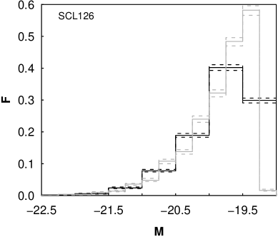
Figure 12.— The differential luminosity function histograms $F=dN/dM$, where $M$ is the absolute magnitude of a galaxy, for galaxies in the supercluster SCL126; here the solid line shows the luminosity function and the dashed lines indicate the Poisson errors. Black lines show the histogram for the 0.5 magnitude bins, gray lines – for the 0.25 magnitude bins.

The MISE is defined as

MISE $$= E\int\left(\hat{f}(x)-f(x)\right)^{2}dx$$ (A1)

$$= \int\mbox{Var}\left(\hat{f}(x)\right)\,dx+\int\left[\mbox{Bias}\left(\hat{f}(x)\right)\right]^{2}dx.$$ (A2)

The two terms in the last equality depend in a different way on the kernel width (bandwidth). When we increase this width, the variance decreases, but the bias increases – this is what happens when we take wider bins for Fig. 12. The ’stats’ package chooses the optimal bandwidth as that which minimizes the MISE. We could also try to minimise the local mean standard error MSE($x$), but this asks for adaptive density estimation (using bandwiths that depend on $x$), and the procedure is much more complex.

For a kernel estimate, when binning is replaced by convolution with a suitable kernel, the minimum MISE is of the order of $n^{-4/5}$, where $n$ is the size of the sample, and the optimal kernel width is of the order of $\hat{\sigma}n^{-1/5}$, where $\hat{\sigma}$ is the estimate of the rms deviation of the data (see, e.g. Silverman, 1986). The expression ’of the order to’ can be mostly read as ’equal to’, as the proportionality coefficients are usually close to unity. This kernel width means that there are about $n\cdot n^{-1/5}=n^{4/5}$ points per kernel – we get our accustomed Poissonian error, but only for the optimal kernel width. However, this is only a rough estimate, as the local error, the mean standard error MSE$(x)$ depends on the true density, being larger in the regions where this density has minima or maxima, and is difficult to estimate. Thus the ’stats’ package does not provide the MSE, and we do not show error bars in our figures.

You can compare histograms and kernel densities in Fig 13. Here we generated a random sample of 1000 values for a weighted sum of two normal distributions, calculated its histogram, and applied the R procedure to obtain the optimized kernel density. The optimal kernel width is 0.36, three times smaller than the bin width; however, the kernel density follows well the smooth true density, and recovers the details much better than the histogram does.

Figure 13.— Comparison of the histogram and kernel density estimates. The true density is shown by a thin line, and the kernel estimate obtained by the R ’stats’ package for a sample of the size 1000 – by a thick line. For comparison, we show a histogram (obtained also by ’R’). It is clearly seen that the histogram is inferior to the kernel estimate.

As the total number of galaxies in our superclusters is large, the differences between the estimated and true densities are small. These differences can be easily estimated. Let us take SCL9 as an example (SCL126 has more galaxies, and the errors are slightly smaller). The total number of galaxies in SCL9 is 1176, so the MISE for the distributions involving the whole supercluster is $\approx 0.0035$, and about 0.006 for separate populations (the corresponding rms errors are 0.06 and 0.08). The local errors (MSE) are, in average, a few times smaller (by the ratio of the total range of a random variable to $\hat{\sigma}$). Our use of a constant width kernel does not allow us to better estimate the local errors, but we can always strictly compare densities, using the full data – the integral distributions (e.g., the Kolmogorov-Smirnov test).

Appendix B Spatial densities

When studying the morphology of superclusters of galaxies, a necessary step is to convert the spatial positions of galaxies into spatial densities. The standard approach is to use kernel densities (see, e.g. Silverman, 1986):

$$\varrho(\mathbf{x})=\sum_{i}K(\mathbf{x-x}_{i};h)m_{i},$$

where the sum is over all galaxies, $\mathbf{x}_{i}$ are the coordinates of the $i$-th galaxy, and $m_{i}$ is its mass (or luminosity, if we are estimating luminosity densities; for number densities we set $m_{i}\equiv 1$). The function $K(\mathbf{x};h)$ is the kernel of the width $h$, and a suitable choice of the kernel determines the quality of the density estimate. If the kernel widths depend either on the coordinate $\mathbf{x}$ or on the position of the $i$-th galaxy, the densities are adaptive.

Kernels have to be normalized and symmetrical:

$$\int K(\mathbf{x};h)dV=1,\qquad\int\mathbf{x}K(\mathbf{x};h)dV=0.$$

For the usual case, when densities are calculated for a spatial grid, good kernels are generated by box splines $B_{J}$ (usually used in $N$-body mass assignment). Box splines have compact support (they are local), and they are interpolating on a grid:

$$\sum_{i}B_{J}(x-i)=1,$$

for any $x$, and a small number of indices that give non-zero values for $B_{J}(x)$. In this paper we restrict us to the popular $B_{3}$ splines:

$$B_{3}(x)=\frac{1}{12}\left[|x-2|^{3}-4|x-1|^{3}+6|x|^{3}-4|x+1|^{3}+|x+2|^{3}\right]$$

(this function is different from zero only in the interval $x\in[-2,2]$). We define the (one-dimensional) $B_{3}$ box spline kernel of width $h=N$ as

$$K_{B}^{(1)}(x;N)=B_{3}(x/N)/N.$$

This kernel preserves the interpolation property (mass conservation) for all kernel widths that are integer multiples of the grid step, $h=N$. The 3-D $K_{B}^{(3)}$ box spline kernel we use is given by the direct product of three one-dimensional kernels:

$$K_{B}(\mathbf{x};N)\equiv K_{B}^{(3)}(\mathbf{x};N)=K_{B}^{(1)})(x;N)K_{B}^{(1)}(y;N)K_{B}^{(1)}(z;N),$$

where $\mathbf{x}\equiv\{x,y,z\}$. Although it is a direct product, it is isotropic to a good degree (to a few per cent in the outer regions).

As seen before, the best (optimal) kernel width is usually determined by minimizing the MISE; in our case this is about 6–8$h$ Mpc^-1. We have defined (see RI) superclusters as density enhancements of a common scale of 8$h$ Mpc^-1, so we will use this value.

Appendix C Minkowski functionals and shapefinders

Consider an excursion set $F_{\phi_{0}}$ of a field $\phi(\mathbf{x})$ (the set of all points where density is larger than a given limit, $\phi(\mathbf{x}\geq\phi_{0}$)). Then, the first Minkowski functional (the volume functional) is the volume of this region (the excursion set):

$$V_{0}(\phi_{0})=\int_{F_{\phi_{0}}}d^{3}x\;.$$ (C1)

The second MF is proportional to the surface area of the boundary $\delta F_{\phi}$ of the excursion set:

$$V_{1}(\phi_{0})=\frac{1}{6}\int_{\delta F_{\phi_{0}}}dS(\mathbf{x})\;,$$ (C2)

(but not the area itself, notice the constant). The third MF is proportional to the integrated mean curvature of the boundary:

$$V_{2}(\phi_{0})=\frac{1}{6\pi}\int_{\delta F_{\phi_{0}}}\left(\frac{1}{R_{1}(\mathbf{x})}+\frac{1}{R_{2}(\mathbf{x})}\right)dS(\mathbf{x})\;,$$ (C3)

where $R_{1}(\mathbf{x})$ and $R_{2}(\mathbf{x})$ are the principal radii of curvature of the boundary. The fourth Minkowski functional is proportional to the integrated Gaussian curvature (the Euler characteristic) of the boundary:

$$V_{3}(\phi_{0})=\frac{1}{4\pi}\int_{\delta F_{\phi_{0}}}\frac{1}{R_{1}(\mathbf{x})R_{2}(\mathbf{x})}dS(\mathbf{x})\;.$$ (C4)

At high (low) densities this functional gives us the number of isolated clumps (voids) in the sample (Martínez et al., 2005; Saar et al., 2007).

As the argument labeling the isodensity surfaces, we chose the (excluded) mass fraction $m_{f}$ – the ratio of the mass in regions with density lower than the density at the surface, to the total mass of the supercluster. When this ratio runs from 0 to 1, the iso-surfaces move from the outer limiting boundary into the center of the supercluster, i.e. the fraction $m_{f}=0$ corresponds to the whole supercluster, and $m_{f}=1$ to its highest density peak.

We use directly only the fourth Minkowski functional in this paper; the other functionals are used to calculate the shapefinders (Sahni et al., 1998; Shandarin et al., 2004). The shapefinders are defined as a set of combinations of Minkowski functionals: $H_{1}=3V/S$ (thickness), $H_{2}=S/C$ (width), and $H_{3}=C/4\pi$ (length). The shapefinders have dimensions of length and are normalized to give $H_{i}=R$ for a sphere of radius $R$. For a convex surface, the shapefinders $H_{i}$ follow the inequalities $H_{1}\leq H_{2}\leq H_{3}$. Oblate ellipsoids (pancakes) are characterized by $H_{1}<<H_{2}\approx H_{3}$, while prolate ellipsoids (filaments) are described by $H_{1}\approx H_{2}<<H_{3}$.

Sahni et al. (1998) also defined two dimensionless shapefinders $K_{1}$ (planarity) and $K_{2}$ (filamentarity): $K_{1}=(H_{2}-H_{1})/(H_{2}+H_{1})$ and $K_{2}=(H_{3}-H_{2})/(H_{3}+H_{2})$.

In the $(K_{1},K_{2})$-plane filaments are located near the $K_{2}$-axis, pancakes near the $K_{1}$-axis, and ribbons along the diagonal, connecting the spheres at the origin with the ideal ribbon at $(1,1)$.

C.1. Algorithms

Different algorithms are used to calculate the Minkowski functionals; here we use a simple grid-based algorithm, based on integral geometry (Crofton’s intersection formula), proposed by Schmalzing and Buchert (Schmalzing et al. (1997)).

To start with, we find the density thresholds for given filling fractions $f$ by sorting the grid densities. This is a common step for all grid-based algorithms. Vertexes with higher densities than the threshold form the excursion set. This set is characterized by its basic sets of different dimensions – points (vertexes), edges formed by two neighbouring points, squares (faces) formed by four edges, and cubes formed by six faces. The algorithm counts the numbers of elements of all basic sets, and finds the values of the Minkowski functionals as

$$V_{0} = a^{3}N_{3}\;,$$

$$V_{1} = a^{2}\left(\frac{2}{9}N_{2}-\frac{2}{3}N_{3}\right)\;,$$

$$V_{2} = a\left(\frac{2}{9}N_{1}-\frac{4}{9}N_{2}+\frac{2}{3}N_{3}\right)\;,$$

$$V_{3} = N_{0}-N_{1}+N_{2}-N_{3}\;,$$ (C5)

where $a$ is the grid step, $N_{0}$ is the number of vertexes, $N_{1}$ is the number of edges, $N_{2}$ is the number of squares (faces), and $N_{3}$ is the number of basic cubes in the excursion set.

Appendix D Clumpiness: morphological templates

In Paper RI we generated a series of empirical models which served us as morphological templates to understand the behaviour of shapefinders. These models showed that the morphological signature of rich superclusters corresponds to a multibranched filament; the simplest model for that was a long filament with short filaments across it. In RI we did not study the fine structure of superclusters as expressed by their clumpiness. In these models the locations of points which mimic positions of galaxies were generated randomly. Thus our empirical models in that paper do not recover completely the inner structure of superclusters.

For this appendix, we generated a series of empirical models to understand better the substructure of superclusters. These models will also help us to determine how well our methods distinguish different types of substructure.

In these models, the overall distribution of points (which mimic individual galaxies) resembles a thin filament with a size $10\times 20\times 100$ (in grid units), as in RI. We place inside this filament a series of clusters, located randomly. Their richness, number and size varies so that the total number of objects is always 1000 or 500 (approximately the number of galaxies in superclusters under study, and in individual galaxy populations). We used the richness values 5, 10 and 20; the number of clusters is, correspondingly, 100, 50 and 25. The size of clusters was 1, 5, and 10 in grid units. Small clusters mimic real groups and clusters, large clusters – overdensity regions. Clusters are located randomly and may overlap, forming additional overdensity regions, as, for example, in cores of superclusters, where also galaxy populations are mixed.

We plot the Euler characteristics and morphological signatures for these models in Figs. 14.

The models used in this figure are as follows. In the first set the number of clusters is 25, each cluster has 20 galaxies in it. The sizes of clusters are 1 and 5. In the third model in this set, these clusters are combined together. In the latter model clusters have the same centre coordinates. Thus the model CL125525 (the combined models CL125 and CL525) mimics the distribution where groups are surrounded by lower density galaxies (e.g., ellipticals by spirals).

In the second set the number of clusters is 50, with 10 member galaxies, and in the combined model, cluster centres again coincide (the models CL150, CL550, and CL150550). In the third set (CL125150 and CL525150) we added to the models with 25 clusters (sizes 1 and 5) the model CL150, to have a smaller number of rich groups and a large number of poor groups, but in this case the centres of groups do not coincide. These models mimic the situation where different populations of galaxies are located in clumps of different richness and size, but in separate systems (partly, since clumps may overlap randomly). We plot here also the curves for a simple filament for comparison.

We do not show in this figure models with 100 small clusters and those with cluster size 10; in all these models the values of $V_{3}$ were smaller than in real superclusters. In the case of large clusters the value of $K_{2}$ becomes too large.

Fig. 14 shows that, first, the morphological signature is recovered correctly by our empirical models. Second, the $V_{3}(m_{f})$ curves for different models are different, showing that they discriminate well different substructure.

Figure 14.— The Euler characteristic (upper row) and the morphological signature $K_{1}$-$K_{2}$ (lower row) for the empirical models. Left panels: $N_{cl}=25$, $N_{gal}=20$ and the size of the clusters is 1 and 5 (in grid units), and the combined model where the centres of clusters coincide. Solid line - model CL125, dashed line - model CL525, and dot-dashed line - model CL125525. Middle panels: $N_{cl}=50$, $N_{gal}=10$ and the size of clusters is 1 and 5 (in grid units), and the combined model where the centres of clusters coincide. Solid line - model CL150, dashed line - model CL550, and dot-dashed line - model CL150550. Right panels: the combined models where the centres do not coincide. ’Fil’ denotes a simple filament with randomly distributed points. Solid line - model CL125150, dashed line - model CL525150, and dot-dashed line - model ’Fil’.

These models show that the supercluster SCL126 is better modelled by a small number of richer/bigger clumps, and the supercluster SCL9 – by a large number of smaller clumps. Clusters overlap, thus the maximum values of $V_{3}$ are smaller than the original numbers of clusters in the models. The case when any population of galaxies is located randomly within the supercluster volume does not correspond to the real distribution of galaxies. Of course, our very simple models in which clusters of one galaxy population are surrounded by low density ”clouds” of galaxies from another population do not recover well the details of clumpiness of different galaxy populations of observed superclusters. In real superclusters, populations of galaxies are more strongly mixed.

References

- Balogh et al. (2004) Balogh, M., Eke, V., Miller, C., et al. 2004, MNRAS, 348, 1355
- Bardelli et al. (2000) Bardelli, S., Zucca, E., Zamorani, G., Moscardini, L., Scaramella, R., 2000, MNRAS, 312, 540
- Basilakos (2003) Basilakos, S. 2003, MNRAS, 344, 602
- Basilakos et al. (2006) Basilakos, S., Plionis, M., Yepes, G., Gottlöber, S., Turchaninov, V. 2006, MNRAS, 365, 539
- Basilakos et al. (2001) Basilakos, S., Plionis, M., Rowan-Robinson, M. 2001, MNRAS, 323, 47
- Belsole et al. (2004) Belsole, E., Pratt, G.W., Sauvageot, J.-L-., Bourdin, H. 2004, A&A, 415, 821
- Blanton et al. (2004) Blanton, M.R., Eisenstein, D., Hogg, D.W., et al. 2004, ApJ, 629, 143
- Blanton et al. (2006) Blanton, M.R., Eisenstein, D., Hogg, D.W., et al. 2006, ApJ, 645, 977
- Caretta et al. (2002) Caretta, C.A., Maia, A.G., Kawasaki, W., & Willmer, C.N.A. 2002, AJ, 123, 1200
- Cole et al. (2005) Cole, S., Percival, W.J., Peacock, J.A., et al. 2005, MNRAS,362, 505
- Colless et al. (2001) Colless, M.M., Dalton, G.B., Maddox, S.J., et al. 2001, MNRAS, 328, 1039
- Colless et al. (2003) Colless, M.M., Peterson, B.A., Jackson, C.A., et al. 2003, (astro-ph/0306581)
- Cross et al. (2001) Cross, N.J.G., Driver, S.P., Couch, W., et al. 2001, MNRAS, 324, 825
- Croton et al. (2005) Croton, D.J., Farrar, G.R., Norberg, P., et al. 2005, MNRAS, 356, 1155
- Croton et al. (2004) Croton, D.J., Gaztañaga, E., Baugh, C.M., et al. 2004, MNRAS, 352, 1232
- Davis & Geller (1976) Davis, M., & Geller, M.J. 1976, ApJ, 208, 13
- De Propris et al. (2003) De Propris, R., et al. (2dF GRS Team) 2003, MNRAS, 342, 725
- De Propris et al. (2004) De Propris, R., et al. (2dF GRS Team) 2004, MNRAS, 351, 125
- Donelly et al. (2001) Donelly, R. H., Forman, W., Jones, C., et al. 2001, ApJ, 562, 254
- Dressler (1980) Dressler, A., 1980, ApJ 236, 351
- Einasto et al. (2006) Einasto, J., Einasto, M., Saar, E. et al. 2006 A&A, 459, L1
- Einasto et al. (2007b) Einasto, J., Einasto, M., Saar, E. et al. 2007b, A&A, 462, 397 (Paper II)
- Einasto et al. (2007c) Einasto, J., Einasto, M., Tago, E. et al. 2007a, A&A, 462, 811 (Paper I)
- Einasto et al. (2005b) Einasto, J., Tago E., Einasto, M., et al. 2005b, A&A, 439, 45
- Einasto (1991) Einasto, M. 1991, MNRAS, 252, 261
- Einasto & Einasto (1987) Einasto, M., & Einasto, J., 1987, MNRAS, 226, 543 (E87)
- Einasto et al. (2003b) Einasto, M., Einasto, J., Müller, V., Heinämäki, P., Tucker, D.L. 2003b, AA 401, 851
- Einasto et al. (2007a) Einasto, M., Einasto, J., Tago, E. et al. 2007c, A&A, 464, 815 (Paper III)
- Einasto et al. (2001) Einasto, M., Einasto, J., Tago, E., Müller, V. & Andernach, H., 2001, AJ, 122, 2222 (E01)
- Einasto et al. (2003a) Einasto, M., Jaaniste, J., Einasto, J., et al. 2003, A&A, 405, 821
- Einasto et al. (2007d) Einasto, M., Saar, E., Liivamägi, L. J. et al., 2007a, A&A, 476, 697 (RI)
- Einasto et al. (2005a) Einasto, M., Suhhonenko, I., Heinämäki, P., Einasto, J., Saar, E. 2005, A&A, 436, 17
- Eke et al. (2004) Eke, V. R., Baugh, C. M., Cole, S., et al. 2004, MNRAS, 348, 866
- Fleenor et al. (2005) Fleenor, M.C., Rose, J.A., Christiansen, W.A. et al. 2005, AJ, 130, 957
- Giovanelli, Haynes & Chincarini (1986) Giovanelli, R., Haynes, M.P., Chincarini, G. L., 1986, ApJ, 300, 77
- Goto et al. (2003) Goto, T, Okamura, S., Sekiguchi, M., et al. 2003, PASJ, 55, 757
- Gott et al. (2008) Gott, J.R., Hambrick, D.C., Vogeley, M.S. et al. 2008, ApJ, 675, 16
- Gott et al. (2005) Gott, J.R., Juric, M., Schleger, D. et al. 2005, ApJ, 624, 463
- Gramann & Suhhonenko (2002) Gramann, M. & Suhhonenko, I. 2002, MNRAS, 337, 1417
- Gray et al. (2004) Gray, M.E., Wolf, C., Meisenheimer, K. et al. 2004, MNRAS,347, L73
- Haines et al. (2006) Haines, C.P., Barbera, C.P., Mercurio, A., et al. 2006, ApJ, 647, L21
- Haines et al. (2006) Haines, C.P., Merluzzi, P., Mercurio, A., et al. 2006, MNRAS, 371, 55
- Haines, Gargiulo & Merluzzi (2008) Haines, C.P., Gargiulo, A., Merluzzi, P., 2008, MN, in press [astro/ph 0707.2361v1]
- Hamilton (1988) Hamilton, A.J.S. 1988, ApJL, 331, L59
- Hikage et al. (2003) Hikage, C., Schmalzing, J., Buchert, T., et al. 2003, PASJ55, 911
- Hilton et al. (2005) Hilton, M., Collins, C., De Propris, R. et al., MNRAS 363, 661
- Hogg et al. (2004) Hogg, D.W., Blanton, M.R., Brinchmann, J., et al. 2004, ApJ, 601, L29
- Hogg et al. (2003) Hogg, D.W., Blanton, M.R., Eisenstein, D.J. et al. 2003, ApJ, 585, L5
- Hoyle et al. (2002) Hoyle, F., et al. 2002, ApJ, 580, 663
- Ihaka & Gentleman (1996) Ihaka, R., & Gentleman, R., 1996, J. of Computational and Graphical Statistics, 5, 299
- Jaaniste et al. (1998) Jaaniste, J., Tago, E., Einasto, M. et al. 1998, A&A, 336, 35
- James, Lewis & Colless (2007) James, J.B., Lewis, G.F. & Colless, M. 2007, MNRAS, 375, 128
- Kennicutt (1992) Kennicutt, R.C., J. 1992, ApJS, 79, 255
- Kofman, Einasto & Linde (1987) Kofman, L.A., Einasto, J., & Linde, A.D. 1987, Nature, 326, 48
- Kolokotronis, Basilakos & Plionis (2002) Kolokotronis, V., Basilakos, S. & Plionis, M. 2002, MNRAS, 331, 1020
- Madgwick et al. (2002) Madgwick, D.S., et al. (the 2dFGRS Team), 2002, MNRAS, 333, 133
- Madgwick et al. (2003b) Madgwick, D.S., Hawkins, E., Lahav, O., et al., 2003b, MNRAS, 344, 847
- Madgwick et al. (2003a) Madgwick, D.S., Somerville, R., Lahav, O., Ellis, R., 2003a, MNRAS, 343, 871
- Martínez et al. (2005) Martínez, V.J., Starck, J.-L., Saar, E., et al., 2005, ApJ, 634, 744
- Mercurio et al. (2006) Mercurio, A., Merluzzi, P., Haines, C.P., et al. 2006, MNRAS, 368, 109
- Metcalfe, N., Godwin, J.G. & Peach, J.V., (1994) Metcalfe, N., Godwin, J.G. & Peach, J.V., 1994, MNRAS, 267, 431
- Mobasher et al. (2005) Mobasher, B., Dickinson, M., Ferguson, H.C., et al. 2005, ApJ, 635, 832
- Moles et al. (2005) Moles, M., Benítez, N., Aguerri, J. A. L., et al., astro-ph/0504545
- Nichol et al. (2006) Nichol, R.C., Sheth, R.K., Suto, Y., et al. 2006, MNRAS, 368, 150
- Norberg et al. (2001) Norberg, P., Baugh, C.M., Hawkins, E., et al. 2001, MNRAS, 328, 64
- Norberg et al. (2002) Norberg, P., Baugh, C.M., Hawkins, E., et al. 2002, MNRAS, 332, 827
- Ouchi et al. (2005) Ouchi, M., Shimasaku, K., Akiyama, M., et al. 2005, ApJ Lett, 620, 1
- Park et al. (2005) Park, C., Choi, Y.-Y., Vogeley, M.S., et al. 2005, ApJ, 633, 11
- Park et al. (2007) Park, C., Choi, Y.-Y., Vogeley, M.S., et al. 2007, ApJ, 658, 898
- Phillipps et al. (1998) Phillipps, S., Driver, S.P., Couch, W.J., Smith, R.M. 1998, ApJL, 498, L119
- Plionis (2004) Plionis, M, 2004, In ”Outskirts of galaxy clusters: intense life in the suburbs”. Proceedings IAU Colloquium No. 195, 2004, ed. A. Diaferio
- Porter & Raychaudhury (2005) Porter, S.C. & Raychaudhury, S. 2005, MNRAS, 364, 1387
- Porter & Raychaudhury (2007) Porter, S.C. & Raychaudhury, S. 2007, MNRAS, 375, 1409
- Proust et al. (2006) Proust, D., Quintana, H., Carrasco, E.R. et al. 2006, A&A, 447, 133
- Quintana et al. (2000) Quintana, H., Carrasco, E.R., Reisenegger, A., 2000, AJ, 120, 511
- Rose et al. (2002) Rose, J.A., Gaba, A.E., Christiansen, W.A., et al., 2002, AJ, 123, 1216
- Saar et al. (2007) Saar, E., Martínez, V.J., Starck, J.-L., Donoho, D.L., 2007, MNRAS, 374, 1030
- Sahni et al. (1998) Sahni V., Sathyaprakash B. S., Shandarin S. 1998, ApJ, 495, L5
- Schmalzing et al. (1997) Schmalzing , J., & Buchert, T., 1997, ApJ, 482, L1
- Scodeggio (2001) Scodeggio, M., 2001, AN, 121, 2413
- Shandarin et al. (2004) Shandarin, S.F., Sheth, J.V. and Sahni, V. 2004, MNRAS, 353, 162
- Sheth et al. (2003) Sheth, J.V., Sahni, V., Shandarin, S.F., and Sathyaprakash, B. 2003, MNRAS, 343, 22
- Silverman (1986) Silverman, B.W. Density Estimation for Statistics and Data Analysis, Chapman & Hall / CRC Press, Boca Raton, 1986
- Small (1998) Small, T.A., Ma, C.-P., Sargent, W.L.W., and Hamilton, D., 1998, ApJ, 492, 45
- Tago et al. (2006) Tago, E., Einasto, J., Saar, E. et al. 2006, AN, 327, 365 (T06)
- Venemans et al. (2004) Venemans, B.P, Röttgering, H.J., Overzier, R.A., et al. 2004, A&A, 424, L17
- Vogeley et al. (2004) Vogeley, M.S., Hoyle, F., Rojas, R.R. et al. 2004, In ”Outskirts of galaxy clusters: intense life in the suburbs”. Proceedings IAU Colloquium No. 195, 2004, ed. A. Diaferio
- Wand and Jones (1995) Wand, M. P., and Jones, M. C. Kernel Smoothing, Chapman & Hall, London, 1995
- Wild et al. (2005) Wild, V., Peacock, J.A., Lahav, O., et al. (the 2dFGRS Team) 2005, MNRAS, 356, 247