The Einstein-Podolsky-Rosen paradox: from concepts to applications

Abstract

This Colloquium examines the field of the EPR Gedankenexperiment, from the original paper of Einstein, Podolsky and Rosen, through to modern theoretical proposals of how to realize both the continuous-variable and discrete versions of the EPR paradox. We analyze the relationship with entanglement and Bell’s theorem, and summarize the progress to date towards experimental confirmation of the EPR paradox, with a detailed treatment of the continuous-variable paradox in laser-based experiments. Practical techniques covered include continuous-wave parametric amplifier and optical fibre quantum soliton experiments. We discuss current proposals for extending EPR experiments to massive-particle systems, including spin-squeezing, atomic position entanglement, and quadrature entanglement in ultra-cold atoms. Finally, we examine applications of this technology to quantum key distribution, quantum teleportation and entanglement-swapping.

Contents

1. I Introduction
2. II The continuous variable EPR paradox
   1. II.1 The 1935 argument: EPR’s “elements of reality”
   2. II.2 Schrödinger’s response: entanglement and separability
3. III Discrete spin variables and Bell’s theorem
   1. III.1 The EPR-Bohm paradox: early EPR experiments
   2. III.2 Bell’s theorem
   3. III.3 Experimental tests of Bell’s theorem
4. IV EPR argument for real particles and fields
   1. IV.1 Inferred Heisenberg inequality: continuous variable case
   2. IV.2 Criteria for the discrete EPR paradox
   3. IV.3 A practical linear-estimate criterion for EPR
   4. IV.4 Experimental criteria for demonstrating the paradox
5. V Theoretical model for a continuous variable EPR Experiment
   1. V.1 Two-mode squeezed states
   2. V.2 Measurement techniques
   3. V.3 Effects of loss and imperfect detectors
6. VI EPR, entanglement and Bell criteria
   1. VI.1 “Steering”
   2. VI.2 Symmetric EPR paradox
   3. VI.3 EPR as a special type of entanglement
   4. VI.4 EPR and Bell’s nonlocality
7. VII Continuous-wave EPR experiments
   1. VII.1 Parametric oscillator experiments
   2. VII.2 Experimental Results
8. VIII Pulsed EPR experiments
   1. VIII.1 Optical fiber experiment
   2. VIII.2 Parametric amplifier experiment
9. IX Spin EPR and atoms
   1. IX.1 Transfer of optical entanglement to atomic ensembles
   2. IX.2 Conditional atom ensemble entanglement
10. X Application of EPR entanglement
    1. X.1 Entanglement-based quantum key-distribution
    2. X.2 Quantum Teleportation and Entanglement Swapping
11. XI Outlook

I Introduction

In 1935, Einstein, Podolsky and Rosen (EPR) originated the famous “EPR paradox” (Einstein et al. (1935)). This argument concerns two spatially separated particles which have both perfectly correlated positions and momenta, as is predicted possible by quantum mechanics. The EPR paper spurred investigations into the nonlocality of quantum mechanics, leading to a direct challenge of the philosophies taken for granted by most physicists. Furthermore, the EPR paradox brought into sharp focus the concept of entanglement, now considered to be the underpinning of quantum technology.

Despite its huge significance, relatively little has been done to directly realize the original EPR Gedankenexperiment. Most published discussion has centred around the testing of theorems by Bell (1964), whose work was derived from that of EPR, but proposed more stringent tests dealing with a different set of measurements. The purpose of this Colloquium is to give a different perspective. We go back to EPR’s original paper, and analyze the current theoretical and experimental status, and implications, of the EPR paradox itself: as an independent body of work.

A paradox is: “a seemingly absurd or self-contradictory statement or proposition that may in fact be true”. The EPR conclusion was based on the assumption of local realism, and thus the EPR argument pinpoints a contradiction between local realism and the completeness of quantum mechanics. This was therefore termed a “paradox” by Schrödinger (1935b), Bohm (1951), Bell (1964) and Bohm and Aharonov (1957). EPR took the prevailing view of their era that local realism must be valid. They argued from this premise that quantum mechanics must be incomplete. With the insight later provided by Bell (1964), the EPR argument is best viewed as the first demonstration of problems arising from the premise of local realism.

The intention of EPR was to motivate the search for a theory “better” than quantum mechanics. However, EPR never questioned the correctness of quantum mechanics, only its completeness. They showed that if a set of assumptions, which we now call local realism, is upheld, then quantum mechanics must be incomplete. Owing to the subsequent work of Bell, we now know what EPR didn’t know: local realism, the “realistic philosophy of most working scientists” (Clauser and Shimony (1978)), is itself in question. Thus, an experimental realization of the EPR proposal provides a way to demonstrate a type of entanglement inextricably connected with quantum nonlocality.

In the sense that the local realistic theory envisaged by them cannot exist, EPR were “wrong”. What EPR did reveal in their paper, however, was an inconsistency between local realism and the completeness of quantum mechanics. Hence, we must abandon at least one of these premises. This was clever, insightful and correct. The EPR paper therefore provides a way to distinguish quantum mechanics as a complete theory from classical reality, in a quantitative sense.

The conclusions of the EPR argument can only be drawn if certain correlations between the positions and momenta of the particles can be confirmed experimentally. The work of EPR, like that of Bell, requires experimental demonstration, since it could be supposed that the quantum states in question are not physically accessible, or that quantum mechanics itself is wrong. It is not feasible to prepare the perfect correlations of the original EPR proposal. Instead, we show that the violation of an inferred Heisenberg Uncertainty Principle – an “EPR inequality” – is eminently practical. These EPR inequalities provide a way to test the incompatibility of local realism, as generalized to a non-deterministic situation, with the completeness of quantum mechanics. Violating an EPR inequality is a demonstration of the EPR paradox.

In a nutshell, we will conclude that EPR experiments provide an important complement to those of Bell. While the conclusions of Bell’s theorem are stronger, the EPR approach is applicable to a greater variety of physical systems. Most Bell tests have been confined to single photon counting measurements with discrete outcomes, whereas recent EPR experiments have involved continuous variable outcomes and high detection efficiencies. This leads to possibilities for tests of quantum nonlocality in new regimes involving massive particles and macroscopic systems. Significantly, new applications in the field of quantum information are feasible.

In this Colloquium, we outline the theory of EPR’s seminal paper, and also provide an overview of more recent theoretical and experimental achievements. We discuss the development of the EPR inequalities, and how they can be applied to quantify the EPR paradox for both spin and amplitude measurements. A limiting factor for the early spin EPR experiments of Wu and Shaknov (1950), Freedman and Clauser (1972), Aspect et al. (1981) and others was the low detection efficiencies, which meant probabilities were surmised using a postselected ensemble of counts. In contrast, the more recent EPR experiments report an amplitude correlation measured over the whole ensemble, to produce unconditionally, on demand, states that give the entanglement of the EPR paradox; although causal separation was not yet achieved. We explain in some detail the methodology and development of these experiments, first performed by Ou et al. (1992).

An experimental realization of the EPR proposal will always imply entanglement, and we analyze the relationship between entanglement, the EPR paradox and Bell’s theorem. In looking to the future, we review recent experiments and proposals involving massive particles, ranging from room-temperature spin-squeezing experiments to proposals for the EPR-entanglement of quadratures of ultra-cold Bose-Einstein condensates. A number of possible applications of these novel EPR experiments have already been proposed, for example in the areas of quantum cryptography and quantum teleportation. Finally, we discuss these, with emphasis on those applications that use the form of entanglement closely associated with the EPR paradox.

II The continuous variable EPR paradox

Einstein et al. (1935) focused attention on the mysteries of the quantum entangled state by considering the case of two spatially separated quantum particles that have both maximally correlated momenta and maximally anti-correlated positions. In their paper entitled “Can Quantum-Mechanical Description of Physical Reality Be Considered Complete?”, they pointed out an apparent inconsistency between such states and the premise of local realism, arguing that this inconsistency could only be resolved through a completion of quantum mechanics. Presumably EPR had in mind to supplement quantum theory with a hidden variable theory, consistent with the “elements of reality” defined in their paper.

After Bohm (1952) demonstrated that a (non-local) hidden-variable theory was feasible, subsequent work by Bell (1964) proved the impossibility of completing quantum mechanics with local hidden variable theories. This resolves the paradox by pointing to a failure of local realism itself – at least at the microscopic level. The EPR argument nevertheless remains significant.

It reveals the necessity of either rejecting local realism or completing quantum mechanics (or both).

II.1 The 1935 argument: EPR’s “elements of reality”

The EPR argument is based on the premises that are now generally referred to as local realism (quotes are from the original paper):

• “If, without disturbing a system, we can predict with certainty the value of a physical quantity”, then “there exists an element of physical reality corresponding to this physical quantity”. The “element of reality” represents the predetermined value for the physical quantity.

• The locality assumption postulates no action-at-a-distance, so that measurements at a location $B$ cannot immediately “disturb” the system at a spatially separated location $A$ .

EPR treated the case of a non-factorizable pure state $|\psi\rangle$ which describes the results for measurements performed on two spatially separated systems at $A$ and $B$ (Fig. 1). “Non-factorizable” means “entangled”, that is, we cannot express $|\psi\rangle$ as a simple product $|\psi\rangle=|\psi\rangle_{A}|\psi\rangle_{B}$, where $|\psi\rangle_{A}$ and $|\psi\rangle_{B}$ are quantum states for the results of measurements at $A$ and $B$, respectively.

In the first part of their paper, EPR point out in a general way the puzzling aspects of such entangled states. The key issue is that one can expand $|\psi\rangle$ in terms of more than one basis, that correspond to different experimental settings, which we parametrize by $\phi$. Consider the state

$$\left|\psi\right\rangle=\int dx\left|\psi_{x}\right\rangle_{\phi,A}\left|u_{x}\right\rangle_{\phi,B}\,.$$ (1)

Here the eigenvalue $x$ could be continuous or discrete. The parameter setting $\phi$ at the detector $B$ is used to define a particular orthogonal measurement basis $\left|u_{x}\right\rangle_{\phi,B}$. On measurement at $B$, this projects out a wave-function $\left|\psi_{x}\right\rangle_{\phi,A}$ at $A$, the process called “reduction of the wave packet”. The puzzling issue is that different choices of measurements $\phi$ at $B$ will cause reduction of the wave packet at A in more than one possible way. EPR state that, “as a consequence of two different measurements” at $B$, the “second system may be left in states with two different wavefunctions”. Yet, “no real change can take place in the second system in consequence of anything that may be done to the first system”.

Despite the apparently acausal nature of state collapse (Herbert (1982)), the linearity or ‘nocloning’ property of quantum mechanics rules out superluminal communication (Dieks (1982); Wootters and Zurek (1982)). This clearly supports EPR’s original insight. Schrödinger (1935b, 1936) studied this case as well, referring to this apparent influence by $B$ on the remote system $A$ as “steering”.

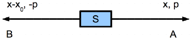
Figure 1: (Color online) The original EPR gedanken-experiment. Two particles move from a source $S$ into spatially separated regions $A$ and $B$, and yet continue to have maximally correlated positions and anti-correlated momenta. This means one may make an instant prediction, with $100$% accuracy, of either the position or momentum of particle $A$, by performing a measurement at $B$. EPR concluded the results of both measurements at $A$ pre-exist, in the form of “elements of reality”, and outlined the premises, local realism, rigorously associated with this reasoning.

The problem was crystallized by EPR with a specific example, shown in Fig. 1. EPR considered two spatially separated subsystems, at $A$ and $B$, each with two observables $\hat{x}$ and $\hat{p}$ where $\hat{x}$ and $\hat{p}$ are non-commuting quantum operators, with commutator $\left[\hat{x},\hat{p}\right]=\hat{x}\hat{p}-\hat{p}\hat{x}=2C\neq 0$. The results of the measurements $\hat{x}$ and $\hat{p}$ are denoted $x$ and $p$ respectively, and this convention we follow throughout the paper. We note that EPR assumed a continuous variable spectrum, but this is not crucial to the concepts they raised. In our treatment we will scale the observables so that $C=i$, for simplicity, which gives rise to the Heisenberg uncertainty relation

$$\Delta x\Delta p\geq 1\,\,.$$ (2)

where $\Delta x$ and $\Delta p$ are the standard deviations in the results $x$ and $p$, respectively.

EPR considered the quantum wavefunction $\psi$ defined in a position representation

$$\psi\left(x,x^{B}\right)=\int e^{\left(ip/\hbar\right)\left(x-x^{B}-x_{0}\right)}dp\,,$$ (3)

where $x_{0}$ is a constant implying space-like separation. Here the pairs $x$ and $p$ refer to the results for position and momentum measurements at $A$, while $x^{B}$ and $p^{B}$ denote the position and momentum measurements at $B$. We leave off the superscript for system $A$, to emphasize the inherent asymmetry that exists in the EPR argument, where one system $A$ is steered by the other, $B$.

According to quantum mechanics, one can “predict with certainty” that a measurement $\hat{x}$ will give result $x^{B}+x_{0}$, if a measurement $\hat{x^{B}}$, with result $x^{B}$, was already performed at $B$. One may also “predict with certainty” the result of measurement $\hat{p}$, for a different choice of measurement at $B$. If the momentum at $B$ is measured to be $p$, then the result for $\hat{p}$ is $-p$. These predictions are made “without disturbing the second system” at $A$, based on the assumption, implicit in the original EPR paper, of “locality”. The locality assumption can be strengthened if the measurement events at $A$ and $B$ are causally separated (such that no signal can travel from one event to the other, unless faster than the speed of light).

The remainder of the EPR argument may be summarized as follows (Clauser and Shimony (1978)). Assuming local realism, one deduces that both the measurement outcomes, for $x$ and $p$ at $A$, are predetermined. The perfect correlation of $x$ with $x^{B}+x_{0}$ implies the existence of an “element of reality” for the measurement $\hat{x}$. Similarly, the correlation of $p$ with $-p^{B}$ implies an “element of reality” for $\hat{p}$. Although not mentioned by EPR, it will prove useful to mathematically represent the “elements of reality” for $\hat{x}$ and $\hat{p}$ by the respective variables $\mu_{x}^{A}$ and $\mu_{p}^{A}$ , whose “possible values are the predicted results of the measurement” (Mermin (1990)).

To continue the argument, local realism implies the existence of two elements of reality, $\mu_{x}^{A}$ and $\mu_{p}^{A}$, that simultaneously predetermine, with absolute definiteness, the results for measurement $x$ or $p$ at $A$. These “elements of reality” for the localized subsystem $A$ are not themselves consistent with quantum mechanics. Simultaneous determinacy for both the position and momentum is not possible for any quantum state. Hence, assuming the validity of local realism, one concludes quantum mechanics to be incomplete. Bohr’s early reply (Bohr (1935)) to EPR was essentially an intuitive defense of quantum mechanics and a questioning of the relevance of local realism.

II.2 Schrödinger’s response: entanglement and separability

It was soon realized that the paradox was intimately related to the structure of the wavefunction in quantum mechanics, and the opposite ideas of entanglement and separability. Schrödinger (1935) pointed out that the EPR two-particle wavefunction in Eq. (3) was verschränkten - which he later translated as entangled (Schrödinger (1935b)) - i.e., not of the separable form $\psi_{A}\psi_{B}$. Both he and Furry (1936) considered as a possible resolution of the paradox that this “entanglement” degrades as the particles separate spatially, so that EPR correlations would not be physically realizable. Experiments considered in this Colloquium show this resolution to be untenable microscopically, but the proposal led to later theories which only modify quantum mechanics macroscopically (Ghirardi et al. (1986); Bell (1988); Bassi and Ghirardi (2003)).

Quantum inseparability (entanglement) for a general mixed quantum state is defined as the failure of

$$\widehat{\rho}=\int d{\lambda}P\left(\lambda\right)\widehat{\rho}_{\lambda}^{A}\otimes\widehat{\rho}_{\lambda}^{B}\,\,,$$ (4)

where $\int d{\lambda}P(\lambda)=1$ and $\widehat{\rho}$ is the density operator. Here $\lambda$ is a discrete or continuous label for component states, and $\widehat{\rho}_{\lambda}^{A,B}$ correspond to density operators that are restricted to the Hilbert spaces $A$,$B$ respectively.

The definition of inseparability extends beyond that of the EPR situation, in that one considers a whole spectrum of measurement choices, parametrized by $\theta$ for those performed on system $A$, and by $\phi$ for those performed on $B$. We introduce the new notation $\hat{x}_{\theta}^{A}$ and $\hat{x}_{\phi}^{B}$ to describe all measurements at $A$ and $B$. Denoting the eigenstates of $\hat{x}_{\theta}^{A}$ by $|x_{\theta}^{A}\rangle$, we define $P_{Q}\left(x_{\theta}^{A}\left|\theta,\lambda\right.\right)=\langle x_{\theta}^{A}|\widehat{\rho}_{\lambda}^{A}|x_{\theta}^{A}\rangle$ and $P_{Q}\left(x_{\phi}^{B}\left|\phi,\lambda\right.\right)=\langle x_{\phi}^{B}|\widehat{\rho}_{\lambda}^{B}|x_{\phi}^{B}\rangle$, which are the localized probabilities for observing results $x_{\theta}^{A}$ and $x_{\phi}^{B}$ respectively. The separability condition (4) then implies that joint probabilities $P(x_{\theta}^{A},x_{\phi}^{B})$ are given as:

$$P\left(x_{\theta}^{A},x_{\phi}^{B}\right)=\int d\lambda P\left(\lambda\right)P_{Q}\left(x_{\theta}^{A}\left|\lambda\right.\right)P_{Q}\left(x_{\phi}^{B}\left|\lambda\right.\right)\,\,.$$ (5)

We note the restriction, that for example $\Delta^{2}(x^{A}|\lambda)\Delta^{2}(p^{A}|\lambda)\geq 1$ where $\Delta^{2}(x^{A}|\lambda)$ and $\Delta^{2}(p^{A}|\lambda)$ are the variances of $P_{Q}\left(x_{\theta}^{A}\left|\theta,\lambda\right.\right)$ for the choices $\theta$ corresponding to position $x$ and momentum $p$, respectively. The original EPR state of Eq. (3) is not separable.

The most precise signatures of entanglement rely on entropic or more general information-theoretic measures. This can be seen in its simplest form when $\widehat{\rho}$ is a pure state, so that $Tr\widehat{\rho}^{2}=1$. Under these conditions, it follows that $\widehat{\rho}$ is entangled if and only if the von Neumann entropy measure of either reduced density matrix $\widehat{\rho}^{A}=Tr_{B}\widehat{\rho}$ or $\widehat{\rho}^{B}=Tr_{A}\widehat{\rho}$ is positive. Here the entropy is defined as:

$$S[\widehat{\rho}]=-Tr\widehat{\rho}\ln\widehat{\rho}$$ (6)

When $\widehat{\rho}$ is a mixed state, one must turn to variational measures like the entanglement of formation to obtain necessary and sufficient measures (Bennett et al. (1996)). The entanglement of formation leads to the popular concurrence measure for two qubits (Wootters (1998)). A necessary but not sufficient measure for entanglement is the partial transpose criterion of Peres (1996).

III Discrete spin variables and Bell’s theorem

III.1 The EPR-Bohm paradox: early EPR experiments

As the continuous-variable EPR proposal was not experimentally realizable at the time, much of the early work relied on an adaptation of the EPR paradox to spin measurements by Bohm (1951), as depicted in Fig. (2).

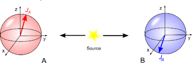
Figure 2: (Color online) The Bohm gedanken EPR experiment. Two spin-$\frac{1}{2}$ particles prepared in a singlet state move from the source into spatially separated regions $A$ and $B$, and give anti-correlated outcomes for $J_{\theta}^{A}$ and $J_{\theta}^{B}$, where $\theta$ is $x$, $y$ or $z$.

This corresponds to the general form given in Eq. (1). Specifically, Bohm considered two spatially-separated spin-$1/2$ particles at $A$ and $B$ produced in an entangled singlet state (often referred to as the “EPR-Bohm state” or the “Bell-state”):

$$\left|\psi\right\rangle=\frac{1}{\sqrt{2}}\left(\left|\frac{1}{2}\right\rangle_{A}\left|-\frac{1}{2}\right\rangle_{B}-\left|-\frac{1}{2}\right\rangle_{A}\left|\frac{1}{2}\right\rangle_{B}\right)$$ (7)

Here $|\pm\frac{1}{2}\rangle_{A}$ are eigenstates of the spin operator $\widehat{J}_{z}^{A}$, and we use $\widehat{J}_{z}^{A}$ , $\widehat{J}_{x}^{A}$ , $\widehat{J}_{y}^{A}$ to define the spin-components measured at location $A$. The spin-eigenstates and measurements at $B$ are defined similarly. By considering different quantization axes, one obtains different but equivalent expansions of $\left|\psi\right\rangle$ in Eq. (1), just as EPR suggested.

Bohm’s reasoning is based on the existence, for Eq. (7), of a maximum anti-correlation between not only $\widehat{J}_{z}^{A}$ and $\widehat{J}_{z}^{B}$, but $\widehat{J}_{y}^{A}$ and $\widehat{J}_{y}^{B}$, and also $\widehat{J}_{x}^{A}$ and $\widehat{J}_{x}^{B}$. An assumption of local realism would lead to the conclusion that the three spin components of particle $A$ were simultaneously predetermined, with absolute definiteness. Since no such quantum description exists, this is the situation of an EPR paradox. A simple explanation of the discrete-variable EPR paradox has been presented by Mermin (1990) in relation to the three-particle Greenberger-Horne-Zeilinger correlation (Greenberger et al. (1989)).

An early attempt to realize EPR-Bohm correlations for discrete (spin) variables came from Bleuler and Bradt (1948), who examined the gamma-radiation emitted from positron annihilation. These are spin-one particles which form an entangled singlet. Here, correlations were measured between the polarizations of emitted photons, but with very inefficient Compton-scattering polarizers and detectors, and no control of causal separation. Several further experiments were performed along similar lines (Wu and Shaknov (1950)), as well as with correlated protons (Lamehi-Rachti and Mittig (1976)). While these are sometimes regarded as demonstrating the EPR paradox (Bohm and Aharonov (1957)), the fact that they involved extremely inefficient detectors, with postselection of coincidence counts, makes this interpretation debatable.

III.2 Bell’s theorem

The EPR paper concludes by referring to theories that might complete quantum mechanics: “..we have left open the question of whether or not such a description exists. We believe, however, that such a theory is possible”. The seminal works of Bell (1964, 1988) and Clauser et al. (1969) (CHSH) clarified this issue, to show that this speculation was wrong. Bell showed that the predictions of local hidden variable theories (LHV) differ from those of quantum mechanics, for the “Bell state”, Eq. (7).

Bell-CHSH considered theories for two spatially-separated subsystems $A$ and $B$. As with separable states, Eq. (4) and Eq. (5), it is assumed there exist parameters $\lambda$ that are shared between the subsystems and which denote localized – though not necessarily quantum – states for each. Measurements can be performed on $A$ and $B$, and the measurement choice is parametrized by $\theta$ and $\phi$, respectively. Thus for example, $\theta$ may be chosen to be either position and momentum, as in the original EPR gedanken experiment, or an analyzer angle as in the Bohm-EPR gedanken experiment. We denote the result of the measurement labelled $\theta$ at $A$ as $x_{\theta}^{A}$, and use similar notation for outcomes at $B$. The assumption of Bell’s locality is that the probability $P\left(x_{\theta}^{A}\left|\lambda\right.\right)$ for $x_{\theta}^{A}$ depends on $\lambda$ and $\theta$, but is independent of $\phi$; and similarly for $P\left(x_{\phi}^{B}\left|\lambda\right.\right)$. The “local hidden variable” assumption of Bell and CHSH then implies the joint probability $P(x_{\theta}^{A},x_{\phi}^{B})$ to be

$$P\left(x_{\theta}^{A},x_{\phi}^{B}\right) = \int_{\lambda}d\lambda P(\lambda)P\left(x_{\theta}^{A}\left|\lambda\right.\right)P\left(x_{\phi}^{B}\left|\lambda\right.\right),$$ (8)

where $P(\lambda)$ is the distribution for the $\lambda$. This assumption, which we call “Bell-CHSH local realism”, differs from Eq. (5) for separability, in that the probabilities $P(x_{\theta}^{A}|\lambda)$ and $P(x_{\phi}^{B}|\lambda)$ do not arise from localised quantum states. From the assumption Eq. (8) of LHV, Bell and CHSH derived constraints, famously referred to as Bell’s inequalities. They showed that quantum mechanics predicts a violation for efficient measurements made on Bohm’s entangled state, Eq. (7).

Bell’s work provided a resolution of the EPR paradox, in the sense that a measured violation would indicate a failure of local realism. While Bell’s assumption of local hidden variables is not formally identical to that of EPR’s local realism, one can be extrapolated from the other (Section VI.A.3). The failure of local hidden variables is then indicative of a failure of local realism.

III.3 Experimental tests of Bell’s theorem

A violation of modified Bell inequalities, that employ auxiliary fair-sampling assumptions (Clauser and Shimony (1978)), has been achieved by Freedman and Clauser (1972), Kasday et al. (1975), Fry and Thompson (1976), Aspect et al. (1981), Shih and Alley (1988), Ou and Mandel (1988) and others. Most of these experiments employ photon pairs created via atomic transitions or using non-linear optical techniques such as optical parametric amplification. These methods provide an exquisite source of highly entangled photons in a Bell-state. Causal separation was achieved by Aspect et al. (1982), with subsequent improvements by Weihs et al. (1998).

However, the low optical and photo-detector efficiencies for counting individual photons ($\sim 5\%$ in the Weihs et al. (1998) experiment) prevent the original Bell inequality from being violated. The original Bell inequality requires a threshold efficiency of $83\%$ ($\eta\sim 0.83)$ per detector (Garg and Mermin (1987); Clauser and Shimony (1978); Fry et al. (1995)), in order to exclude all local hidden variable theories. For lower efficiencies, one can construct local hidden variable theories to explain the observed correlations (Clauser and Horne (1974); Larsson (1999)). Nevertheless, these experiments, elegantly summarized by Zeilinger (1999) and Aspect (2002), exclude the most appealing local realistic theories and thus represent strong evidence in favor of abandoning the local realism premise.

While highly efficient experimental violations of Bell’s inequalities in ion traps (Rowe et al. (2001)) have been reported, these have been limited to situations of poor spatial separation between measurements on subsystems. A conclusive experiment would require both high efficiency and causal separations, as suggested by Kwiat et al. (1994), and Fry et al. (1995). Reported system efficiencies are currently up to $51\%$ (U’Ren et al. (2004)), while typical photo-diode single-photon detection efficiencies are now $60\%$ or more (Polyakov and Migdall (2007)), and further improvements up to $88\%$ with more specialized detectors (Takeuchi et al. (1999)) makes a future loophole-free experiment not impossible.

IV EPR argument for real particles and fields

In this Colloquium, we focus on the realization of the original EPR paradox. To recreate the precise gedanken proposal of EPR, one needs perfect correlations between the positions of two separated particles, and also between their momenta. This is physically impossible, in practice.

In order to demonstrate the existence of EPR correlations for real experiments, one therefore needs to minimally extend the EPR argument, in particular their definition of local realism, to situations where there is less than perfect correlation. We point out that near perfect correlation of the detected photon pairs has been achieved in the seminal “a posteriori” realization of the EPR gedanken experiment by Aspect et al. (1981). However, it is debatable whether this can be regarded as a rigorous EPR experiment, because for the full ensemble, most counts at one detector correspond to no detection at the other.

The stochastic extension of EPR’s local realism is that one can predict with a specified probability distribution repeated outcomes of a measurement, remotely, so the “values” of the elements of reality are in fact those probability distributions. This definition is the meaning of “local realism” in the text below. As considered by Furry (1936) and Reid (1989), this allows the derivation of an inequality whose violation indicates the EPR paradox.

We consider non-commuting observables associated with a subsystem at $A$, in the realistic case where measurements made at $B$ do not allow the prediction of outcomes at $A$ to be made with certainty. Like EPR, we assume causal separation of the observations and the validity of quantum mechanics. Our approach applies to any non-commuting observables, and we focus in turn on the continuous variable and discrete cases.

IV.1 Inferred Heisenberg inequality: continuous variable case

Suppose that, based on a result $x^{B}$ for the measurement at $B$, an estimate $x_{est}\left(x_{B}\right)$ is made of the result $x$ at $A$. We may define the average error $\Delta_{inf}x$ of this inference as the root mean square (RMS) of the deviation of the estimate from the actual value, so that

$$\Delta_{inf}^{2}x=\int dxdx^{B}P\left(x,x_{B}\right)\left(x-x_{est}\left(x_{B}\right)\right)^{2}\,\,.$$ (9)

An inference variance $\Delta_{inf}^{2}p$ is defined similarly.

The best estimate, which minimizes $\Delta_{inf}x$, is given by choosing $x_{est}$ for each $x^{B}$ to be the mean $\langle x|x^{B}\rangle$ of the conditional distribution $P\left(x\left|x^{B}\right.\right)$. This is seen upon noting that for each result $x^{B}$, we can define the RMS error in each estimate as

$$\Delta_{inf}^{2}\left(x\left|x^{B}\right.\right)\,=\int dxP\left(x\left|x^{B}\right.\right)\left(x-x_{est}\left(x^{B}\right)\right)^{2}\,\,.$$ (10)

The average error in each inference is minimized for $x_{est}=\langle x|x^{B}\rangle\,$, when each $\Delta_{inf}^{2}\left(x\left|x^{B}\right.\right)\,$ becomes the variance $\Delta^{2}(x|x^{B})$ of $P\left(x\left|x^{B}\right.\right)$.

We thus define the minimum inference error $\Delta_{inf}x$ for position, averaged over all possible values of $x^{B}$, as

$$V_{A|B}^{x} = \Delta_{inf}^{2}x\Bigl{|}_{min}=\int dx^{B}P\left(x^{B}\right)\Delta^{2}\left(x\left|x^{B}\right.\right)\,\,,$$ (11)

where $P\left(x^{B}\right)$ is the probability for a result $x^{B}$ upon measurement of $\hat{x}^{B}.$ This minimized inference variance is the average of the individual variances for each outcome at $B$. Similarly, we can define a minimum inference variance, $V_{A|B}^{p}$ , for momentum.

We now derive the EPR criterion applicable to this more general situation. We follow the logic of the original argument, as outlined in Section II. Referring back to Fig. (1), we remember that if we assume local realism, there will exist a predetermination of the results for both $x$ and $p$. In this case, however, the predetermination is probabilistic, because we cannot “predict with certainty” the result $x$. We can predict the probability for $x$ however, based on remote measurement at $B$. We recall the “element of reality” is a variable, ascribed to the local system $A$, as part of a theory, to quantify this predetermination. The “element of reality” $\mu_{x}^{A}$ associated with $\hat{x}$ is, in the words of Mermin (1990) that “predictable value” for a measurement at $A$, based on a measurement at $B$, which “ought to exist whether or not we actually carry out the procedure necessary for its prediction, since this in no way disturbs it”. Given the EPR premise and our extension of it, we deduce that “elements of reality” still exist, but the “predictable values” associated with them are now probability distributions.

This requires an extension to the definition of the element of reality. As before, the $\mu_{x}^{A}$ is a variable which takes on certain values, but the values no longer represent a single predicted outcome for result $x$ at $A$, but rather they represent a predicted probability distribution for the results $x$ at $A$. Thus each value for $\mu_{x}^{A}$ defines a probability distribution for $x$. Since the set of predicted distributions are the conditionals $P(x|x^{B})$, one for each value of $x^{B}$, the logical choice is to label the element of reality by the outcomes $x^{B}$, but bearing in mind the set of predetermined results is not the set $\bigl{\{}x^{B}\bigr{\}}$, but is the set of associated conditional distributions $\bigl{\{}P(x|x^{B})\bigr{\}}$. Thus we say if the element of reality $\mu_{x}^{A}$ takes the value $x^{B}$, then the predicted outcome for $x$ is given probabilistically as $P(x|x^{B})$.

Such probability distributions are also implicit in the extensions by Clauser et al. (1969) and Bell (1988) of Bell’s theorem to systems of less-than-ideal correlation. The $P(x_{\theta}^{A}|\lambda)$ used in Eq. (8) is the probability for a result at $A$ given a hidden variable $\lambda$. The “element of reality” and “hidden variable” have similar meanings, except that the element of reality is a special “hidden variable” following from the EPR logic.

To recap the argument, we define $\mu_{x}^{A}$ as a variable whose values, mathematically speaking, are the set of possible outcomes $x^{B}$. We also define $P(x|\mu_{x}^{A})$ as the probability of observing the value $x$ for the measurement $\hat{x}$, in a system $A$ specified by the ‘element of reality’ $\mu_{x}^{A}$. We might also ask, what is the probability that the element of reality has a certain value, namely, what is $P(\mu_{x}^{A})$? Clearly, a particular value for $\mu_{x}^{A}$ occurs with probability $P\left(\mu_{x}^{A}\right)=P(x^{B})$. This is because in the local realism framework, the action of measurement at $B$ (to get outcome $x^{B}$) cannot create the value of the element of reality $\mu_{x}^{A}$, yet it informs us of its value.

An analogous reasoning will imply probabilistic elements of reality for $p$ at $A$, with the result that two elements of reality $\mu_{x}^{A},\mu_{p}^{A}$ are introduced to simultaneously describe results for the localized system $A$. We introduce a joint probability distribution $P(\mu_{x}^{A},\mu_{p}^{A})$ for the values assumed by these elements of reality.

It is straightforward to show from the definition of Eq (11) that if $V_{A|B}^{x}V_{A|B}^{p}<1$, then the pair of elements of reality for $A$ cannot be consistent with a quantum wave-function. This indicates an inconsistency of local realism with the completeness of quantum mechanics. To do this, we quantify the statistical properties of the elements of reality by defining $\Delta^{2}\left(x|\mu_{x}^{A}\right)$ and $\Delta^{2}\left(p|{\mu}_{p}^{A}\right)$ as the variances of the probability distributions $P(x|\mu_{x}^{A})$ and $P(p|\mu_{p}^{A})$. Thus the measurable inference variance is a measure of the average indeterminacy:

$$V_{A|B}^{x} = \int d{\mu_{x}^{A}}P(\mu_{x}^{A})\Delta^{2}\left(x|\mu_{x}^{A}\right)$$

$$= \int d\mu_{x}^{A}d\mu_{p}^{A}P(\mu_{x}^{A},\mu_{p}^{A})\Delta^{2}\left(x|\mu_{x}^{A}\right)$$

(similarly for $V_{A|B}^{p}$ and $\Delta_{inf}^{2}p$). The assumption that the state depicted by a particular pair $\mu_{x}^{A}$, $\mu_{p}^{A}$ has an equivalent quantum description demands that the conditional probabilities satisfy the same relations as the probabilities for a quantum state. For example, if $x$ and $p$ satisfy $\Delta x\Delta p\geq 1$, then $\Delta\left(x|\mu_{x}^{A}\right)\Delta\left(p|{\mu}_{p}^{A}\right)\geq 1$. Simple application of the Cauchy-Schwarz inequality gives

$$\Delta_{inf}x\Delta_{inf}p \geq V_{A|B}^{x}V_{A|B}^{p}$$

$$= \langle\Delta^{2}\left(x|\mu_{x}^{A}\right)\rangle\langle\Delta^{2}\left(p|\mu_{p}^{A}\right)\rangle$$

$$\geq |\langle\Delta\left(x|\mu_{x}^{A}\right)\Delta\left(p|\mu_{p}^{A}\right)\rangle|^{2}\geq 1$$

Thus the observation of $V_{A|B}^{x}V_{A|B}^{p}<1$, or more generally,

$$\Delta_{inf}x\Delta_{inf}p<1$$ (14)

is an EPR criterion, meaning that this would imply an EPR paradox (Reid (1989, 2004)).

One can in principle use any quantum uncertainty constraint (Cavalcanti and Reid (2007)). Take for example, the relation $\Delta^{2}\left(x|\mu_{x}^{A}\right)+\Delta^{2}\left(p|{\mu}_{p}^{A}\right)\geq 2$, which follows from that of Heisenberg. From this we derive $V_{A|B}^{x}+V_{A|B}^{p}\geq 2$, to imply that

$$\Delta_{inf}^{2}x+\Delta_{inf}^{2}p<2$$ (15)

is also an EPR criterion. On the face of it, this is less useful; since if (15) holds, then (14) must also hold.

IV.2 Criteria for the discrete EPR paradox

The discrete variant of the EPR paradox was treated in Section III. Conclusive experimental realization of this paradox needs to account for imperfect sources and detectors, just as in the continuous variable case.

Criteria sufficient to demonstrate Bohm’s EPR paradox can be derived with the inferred uncertainty approach. Using the Heisenberg spin uncertainty relation $\Delta J_{x}^{A}\Delta J_{y}^{A}\geq\left|\left\langle J_{z}^{A}\right\rangle\right|/2$, one obtains (Cavalcanti and Reid (2007)) the following spin-EPR criterion that is useful for the Bell state Eq. (7):

$$\Delta_{inf}J_{x}^{A}\Delta_{inf}J_{y}^{A} < \frac{1}{2}\sum_{{J_{z}^{B}}}P\left(J_{z}^{B}\right)\left|\left\langle J_{z}^{A}\right\rangle_{J_{z}^{B}}\right|\,\,.$$ (16)

Here $\left\langle J_{z}^{A}\right\rangle_{J_{z}^{B}}$ is the mean of the conditional distribution $P\left(J_{z}^{A}|J_{z}^{B}\right)$. Calculations for Eq. (7) including the effect of detection efficiency $\eta$ reveals this EPR criterion to be satisfied for $\eta>0.62$. Further spin-EPR inequalities have recently been derived (Cavalcanti et al. (2007a)), employing quantum uncertainty relations involving sums, rather than the products (Hofmann and Takeuchi (2003)). A constraint on the degree of mixing that can still permit an EPR paradox for the Bell state of Eq. (7) can be deduced from an analysis by Wiseman et al. (2007). These authors report that the Werner (1989) state $\rho_{w}=(1-p_{W})\frac{\mathbb{I}}{4}+p_{W}|\psi\left\rangle\right\langle\psi|$, which is a mixed Bell state, requires $p_{W}>0.5$ to demonstrate “steering”, which we show in Section VI.A is a necessary condition for the EPR paradox.

The concept of spin-EPR has been experimentally tested in the continuum limit with purely optical systems for states where $\left\langle J_{z}^{A}\right\rangle\neq 0$. In this case the EPR criterion, linked closely to a definition of spin squeezing (Kitagawa and Ueda (1993); Sørensen et al. (2001); Korolkova et al. (2002); Bowen et al. (2002a)),

$$\Delta_{inf}J_{x}^{A}\Delta_{inf}J_{y}^{A}<\frac{1}{2}\left|\left\langle J_{z}^{A}\right\rangle\right|$$ (17)

has been derived by Bowen et al. (2002b), and used to demonstrate the EPR paradox, as summarized in Section VII. Here the correlation is described in terms of Stokes operators for the polarization of the fields. The experiments take the limit of large spin values to make a continuum of outcomes, so high efficiency detectors are used.

We can now turn to the question of whether existing spin-half or two-photon experiments were able to conclusively demonstrate an EPR paradox. This depends on the overall efficiency, as in the Bell inequality case. Generating and detecting pairs of photons is generally rather inefficient, although results of up to $51\%$ were reported by U’Ren et al. (2004). This is lower than the $62\%$ threshold given above. We conclude that efficiencies for these types of discrete experiment are still too low, although there have been steady improvements. The required level appears feasible as optical technologies improve.

IV.3 A practical linear-estimate criterion for EPR

It is not always easy to measure conditional distributions. Nevertheless, an inference variance, which is the variance of the conditional distribution, has been so measured for twin beam intensity distributions by Zhang et al. (2003b), who achieved $\Delta_{inf}^{2}$x=0.62.

It is also possible to demonstrate an EPR correlation using criteria based on the measurement of a sufficiently reduced noise in the appropriate sum or difference $x-gx^{B}$ and $p+g^{\prime}p^{B}$ (where here $g$, $g^{\prime}$ are real numbers). This was proposed by Reid (1989) as a practical procedure for measuring EPR correlations.

Suppose that an estimate $x_{est}$ of the result for $\hat{x}$ at $A$, based on a result $x^{B}$ for measurement at $B$, is of the linear form $x_{est}=gx^{B}+d$. The best linear estimate $x_{est}$ is the one that will minimize

$$\Delta_{inf}^{2}x=\left\langle\left\{x-\left(gx^{B}+d\right)\right\}^{2}\right\rangle$$ (18)

The best choices for $g$ and $d$ minimize $\Delta_{inf}^{2}x$ and can be adjusted by experiment, or calculated by linear regression to be $d=\left\langle x-gx^{B}\right\rangle$, $g=\left\langle x,x^{B}\right\rangle/\Delta^{2}x^{B}$ (where we define $\left\langle x,x^{B}\right\rangle=\left\langle xx^{B}\right\rangle-\left\langle x\right\rangle\left\langle x^{B}\right\rangle\,$). There is also an analogous optimum for the value of $g^{\prime}$. This gives a predicted minimum (for linear estimates) of

$$\Delta_{inf}^{2}x\mid_{min,L}=\Delta^{2}\left(x-gx^{B}\right)=\Delta^{2}x-\frac{\langle x,x^{B}\rangle^{2}}{\Delta^{2}x^{B}}$$ (19)

We note that for Gaussian states (Section VI) this best linear estimate for $x$, given $x^{B}$, is equal to the mean of the conditional distribution $P(x|x^{B})$, so that $\Delta_{inf}^{2}x\Bigl{|}_{min,L}=V{}_{A|B}^{x}$ where $V_{A|B}^{x}$ is the variance of the conditional distribution, and this approach thus automatically gives the minimum possible $\Delta_{inf}x$.

The observation of

$$\Delta^{2}\left(x-gx^{B}\right)\Delta^{2}\left(p+g^{\prime}p^{B}\right)<1$$ (20)

is sufficient to imply Eq. (23), which is the condition for the correlation of the original EPR paradox. This was first experimentally achieved by Ou et al. (1992).

We note it is also possible to present an EPR criterion in terms of the sum of the variances. Using (15), on putting $\Delta_{inf}^{2}x=\Delta^{2}\left(x-gx^{B}\right)$ and $\Delta_{inf}^{2}p=\Delta^{2}\left(p+g^{\prime}p^{B}\right)$ we arrive at the linear EPR criterion

$$\Delta^{2}(x-gx^{B})+\Delta^{2}(p+g^{\prime}p^{B})<2.$$ (21)

Strictly speaking, to carry out a true EPR gedanken experiment, one must measure, preferably with causal separation, the separate values for the EPR observables $x$, $x^{B}$, $p$ and $p^{B}$.

IV.4 Experimental criteria for demonstrating the paradox

We now summarize experimental criteria sufficient to realize the EPR paradox. To achieve this, one must have two spatially separated subsystems at $A$ and $B$.

(1): First, to realize the EPR paradox in the spirit intended by EPR it is necessary that measurement events at $A$ and $B$ be causally separated. This point has been extensively discussed in literature on Bell’s inequalities and is needed to justify the locality assumption, given that EPR assumed idealized instantaneous measurements. If $c$ is the speed of light and $t_{A}$ and $t_{B}$ are the times of flight from the source to A and B, then the measurement duration $\Delta t$, time for the measurements at $A$ and $B$ and the separation $L$ between the subsystems must satisfy

$$L>c(t_{A}-t_{B}+\Delta t).$$ (22)

(2): Second, one establishes a prediction protocol, so that for each possible outcome of a measurement at $B$, one can make a prediction about the outcome at $A$. There must be a sufficient correlation between measurements made at $A$ and $B$. The EPR correlation is demonstrated when the product of the average errors in the inferred results $x_{est}$ and $p_{est}$ for $\hat{x}$ and $\hat{p}$ at $A$ falls below a bound determined by the corresponding Heisenberg Uncertainty Principle.

In the continuous variable case where $x$ and $p$ are such that $\Delta x\Delta p\geq 1$ this amounts to

$$\mathcal{E}=\Delta_{inf}x\Delta_{inf}p<1,$$ (23)

where we introduce for use in later sections a symbol $\mathcal{E}$ for the measure of the inference (conditional variance) product $\Delta_{inf}x\Delta_{inf}p$. Similar criteria hold for discrete spin variables.

V Theoretical model for a continuous variable EPR Experiment

V.1 Two-mode squeezed states

As a physically realizable example of the original continuous variable EPR proposal, suppose the two systems $A$ and $B$ are localized modes of the electromagnetic field, with frequencies $\omega_{A,B}$ and boson operators $\widehat{a}$ and $\widehat{b}$ respectively. These can be prepared in an EPR-correlated state using parametric down conversion (Reid and Drummond (1988, 1989); Drummond and Reid (1990)). Using a coherent pump laser at frequency $\omega_{A}+\omega_{B}$, and a nonlinear optical crystal which is phase-matched at these wavelengths, energy is transferred to the modes. As a result, these modes become correlated.

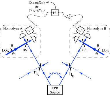
Figure 3: (Color online) Schematic diagram of the measurement of the EPR paradox using field quadrature phase amplitudes. Spatially separated fields $A$ and $B$ radiate outwards from the EPR source, usually Eq. (24). The field quadrature amplitudes are symbolised $Y$ and $X$. The fields combine with an intense local oscillator $LO$ field, at beam splitters $BS$. The outputs of each BS are detected by photodiodes and their difference current is proportional to the amplitude $Y$ or $X$, depending on the phase shift $\theta$. A gain $g$ is introduced to read out the final conditional variances, Eq. (30). Here $\eta_{A}$ and $\eta_{B}$ are the non-ideal efficiencies that model losses, defined in Section V.

The parametric coupling can be described conceptually by the interaction Hamiltonian $H_{I}=i\hbar\kappa(\widehat{a}^{\dagger}\widehat{b}^{\dagger}-\widehat{a}\widehat{b})$, which acts for a finite time $t$ corresponding to the transit time through the nonlinear crystal. For vacuum initial states $|0,0\rangle$ this interaction generates two-mode squeezed light (Caves and Schumaker (1985)), which corresponds to a quantum state in the Schrödinger picture of:

$$\left|\psi\right\rangle = \sum_{{n=0}}^{\infty}c_{n}\left|n\right\rangle_{A}\left|n\right\rangle_{B}$$ (24)

where $c_{n}=\tanh^{n}r/\cosh\,r$ , $r=\kappa t$, and $|n\rangle$ are number states. The parameter $r$ is called the squeezing parameter. The expansion in terms of number states is an example of a Schmidt decomposition, where the pure state is written with a choice of basis that emphasizes the correlation that exists, in this case between the photon numbers of modes $a$ and $b$. The Schmidt decomposition, which is not unique, is a useful tool for identifying the pairs of EPR observables (Ekert and Knight (1995); Huang and Eberly (1993); Law et al. (2000)).

In our case, the EPR observables are the quadrature phase amplitudes, as follows:

$$\hat{x} = \hat{x}^{A}=\widehat{a}^{\dagger}+\widehat{a},$$

$$\hat{p} = \widehat{Y}^{A}=i\left(\widehat{a}^{\dagger}-\widehat{a}\right),$$

$$\hat{x}^{B} = \hat{x}^{B}=\widehat{b}^{\dagger}+\widehat{b},$$

$$\hat{p}^{B} = \widehat{Y}^{B}=i\left(\widehat{b}^{\dagger}-\widehat{b}\right).$$ (25)

The Heisenberg uncertainty relation for the orthogonal amplitudes is $\Delta X^{A}\Delta Y^{A}\geq 1$. Operator solutions at time $t$ can be calculated directly from $H_{I}$ using the rotated Heisenberg picture, to get

$$X^{A(B)}(t) = X^{A(B)}(0)\cosh\left(r\right)+X^{B(A)}(0)\sinh\left(r\right)$$

$$Y^{A(B)}(t) = Y^{A(B)}(0)\cosh\left(r\right)-Y^{B(A)}(0)\sinh\left(r\right)$$ (26)

where $X^{A(B)}(0)$, $Y^{A(B)}(0)$ are the initial “input” amplitudes. As $r\rightarrow\infty$, $X^{A}=X^{B}$ and $Y^{A}=-Y^{B}$, which implies a “squeezing” of the variances of the sum and difference quadratures, so that $\Delta^{2}(X^{A}-X^{B})<2$ and $\Delta^{2}(Y^{A}+Y^{B})<2$. The correlation of $X^{A}$ with $X^{B}$ and the anti-correlation of $P_{A}$ with $P_{B}$, that is the signature of the EPR paradox, is transparent, as $r\rightarrow\infty$.

The “EPR” state Eq. (24) is an example of a bipartite Gaussian state, a state whose Wigner function has a Gaussian form

$$W(\mathbf{x})=\frac{1}{(2\pi)^{2}\sqrt{|\mathbf{C}|}}exp[-\frac{1}{2}(\mathbf{x}-\mu)^{T}\mathbf{C}^{-1}(\mathbf{x}-\mu)]$$ (27)

where $\mathbf{x}=(x_{1},...,x_{4})\equiv(x,p,x^{B},p^{B})$ and we define the mean $\mathbf{\mathbf{\mathbf{\mathbf{\mathbf{\mu}}}}}=\langle\mathbf{x}\rangle$ and the covariance matrix $\mathbf{C}$, such that $C_{ij}=\langle\hat{x}_{{i}},\hat{x}_{{j}}\rangle=\langle x_{i},x_{j}\rangle$, $\langle v,w\rangle=\langle vw\rangle-\langle v\rangle\langle w\rangle$. We note the operator moments of the $\hat{x}_{{i}}$ correspond directly to the corresponding c-number moments. The state (24) yields $\mu=0$ and covariance elements $C_{ii}=\Delta^{2}x_{i}=\cosh\left(2r\right)$, $C_{13}=\langle x,x^{B}\rangle=-C_{24}=-\langle p,p^{B}\rangle=\sinh\left(2r\right)$.

We apply the linear EPR criterion of Section IV.3. For the Gaussian states, in fact the best linear estimate $x_{est}$ for $x$, given $x^{B}$, and the minimum inference variance $\Delta_{inf}^{2}x$ correspond to the mean and variance of the appropriate conditionals, $P(x|x^{B})$ (similarly for $p$). This mean and variance are given as in Section IV.3. The two-mode squeezed state predicts, with $g=g^{\prime}=\tanh\left(2r\right)$,

$$\Delta_{inf}^{2}x=\Delta_{inf}^{2}p=1/\cosh\left(2r\right)\,\,.$$ (28)

Here $x=X^{A}$ is correlated with $X^{B}$, and $p=Y^{A}$ is anti-correlated with $Y^{B}$. EPR correlations are predicted for all nonzero values of the squeeze parameter $r$, with maximum correlations at infinite $r$.

Further proposals for the EPR paradox that use the linear criterion, Eq. (20), have been put forward by Tara and Agarwal (1994). Giovannetti et al. (2001) have presenting an exciting scheme for demonstrating the EPR paradox for massive objects using radiation pressure acting on an oscillating mirror.

V.2 Measurement techniques

Quadrature phase amplitudes can be measured using homodyne detection techniques developed for the detection of squeezed light fields. In the experimental proposal of Drummond and Reid (1990), carried out by Ou et al. (1992), an intracavity nondegenerate downconversion scheme was used. Here the output modes are multi-mode propagating quantum fields, which must be treated using quantum input-output theory (Collett and Gardiner (1984); Gardiner and Zoller (2000); Drummond and Ficek (2004)). Single time-domain modes are obtained through spectral filtering of the photo-current. These behave effectively as described in the simple model given above, together with corrections for cavity detuning and nonlinearity that are negligible near resonance, and not too close to the critical threshold (Dechoum et al. (2004)).

At each location $A$ or $B$, a phase-sensitive, balanced homodyne detector is used to detect the cavity output fields, as depicted in Fig. 3. Here the field $\widehat{a}$ is combined (using a beam splitter) with a very intense “local oscillator” field, modeled classically by the amplitude $E$, and a relative phase shift $\theta$, introduced to create in the detector arms the fields $\widehat{a}_{\pm}=(\widehat{a}\pm Ee^{i\theta})/\sqrt{2}$ . Each field is detected by a photodetector, so that the photocurrent $i_{\pm}^{A}$ is proportional to the incident field intensity $\widehat{a}_{\pm}^{\dagger}\widehat{a}_{\pm}$. The difference photocurrent $i_{D}^{A}=i_{X}^{A}-i_{Y}^{A}$ gives a reading which is proportional to the quadrature amplitude $X_{\theta}^{A}$,

$$i_{D}^{A}\propto E\hat{x}_{\theta}^{A}=E(\widehat{a}^{\dagger}e^{i\theta}+\widehat{a}e^{-i\theta})\,\,.$$ (29)

The choice $\theta=0$ gives a measurement of $X^{A}$, while $\theta=\pi/2$ gives a measurement of $Y^{A}$. The fluctuation in the difference current is, according to the quantum theory of detection, directly proportional to the fluctuation of the field quadrature: thus, $\Delta^{2}i_{D}^{A}$ gives a measure proportional to the variance $\Delta^{2}X_{\theta}^{A}$. A single frequency component of the current must be selected using Fourier analysis in a time-window of duration $\Delta t$, which for causality should be less than the propagation time, $L/c$.

A difference photocurrent $i_{D}^{B}$ defined similarly with respect to the detectors and fields at $B$, gives a measure of $\hat{x}_{\phi}^{B}=\widehat{b}^{\dagger}e^{i\phi}+\widehat{b}e^{-i\phi}$. The fluctuations in $X_{\theta}^{A}-gX_{\phi}^{B}$ are proportional to those of the difference current $i_{D}^{A}-gi_{D}^{B}$ where $g=g^{B}/g^{A}$, and $g^{I}$ indicates any amplification of the current $i^{I}$ before subtraction of the currents. The variance $\Delta^{2}(i_{D}^{A}-gi_{D}^{B})$ is then proportional to the variance $\Delta^{2}(X_{\theta}^{A}-gX_{\phi}^{B})$, so that

$$\Delta^{2}(i_{D}^{A}-gi_{D}^{B})\propto\Delta^{2}(X_{\theta}^{A}-gX_{\phi}^{B})\,\,.$$ (30)

In this way the $\Delta_{inf}^{2}$ of Eq. (23) can be measured. A causal experiment can be analyzed using a time-dependent local oscillator (Drummond (1990)).

V.3 Effects of loss and imperfect detectors

Crucial to the validity of the EPR experiment is the accurate calibration of the correlation relative to the vacuum limit. In optical experiments, this limit is the vacuum noise level as defined within quantum theory. This is represented as $1$ in the right-hand side of the criteria in Eqs. (23) and (20).

The standard procedure for determining the vacuum noise level in the case of quadrature measurements is to replace the correlated state of the input field $\widehat{a}$ at $A$ with a vacuum state $|0\rangle.$ This amounts to removing the two-mode squeezed vacuum field that is incident on the beam-splitter at location $A$ in Fig. 3, and measuring only the fluctuation of the current at $A$. The difference photocurrent $i_{D}^{A}$ is then proportional to the vacuum amplitude and the variance $\Delta^{2}i_{D}^{A}$ is calibrated to be $1$.

To provide a simple but accurate model of detection inefficiencies, we consider an imaginary beam splitter (Fig. 3) placed before the photodetector at each location $A$ and $B$, so that the detected fields $\widehat{a}$ at $A$ and $\widehat{b}$ at $B$ are the combinations $\widehat{a}=\sqrt{\eta_{A}}\widehat{a}_{0}+\sqrt{1-\eta_{A}}\widehat{a}_{vac}$ and $\widehat{b}=\sqrt{\eta_{B}}\widehat{b}_{0}+\sqrt{1-\eta_{B}}\widehat{b}_{vac}$ . Here $\widehat{a}_{vac}$ and $\widehat{b}_{vac}$ represent uncorrelated vacuum mode inputs, $\widehat{a}_{0}$ and $\widehat{b}_{0}$ are the original fields and $\eta_{A/B}$ gives the fractional homodyne efficiency due to optical transmission, mode-matching and photo-detector losses at $A$ and $B$ respectively. Details of the modeling of the detection losses were also discussed by Ou et al. (1992b). Since the loss model is linear, the final state, although no longer pure, is Gaussian, Eq. (27). Thus results concerning necessary and sufficient conditions for entanglement/ EPR that apply to Gaussian states remain useful. This model for loss has been experimentally tested by Bowen et al. (2003a).

The final EPR product where the original fields are given by the two-mode squeezed state, Eq. (24), is

$$\Delta_{inf}X^{A}\Delta_{inf}Y^{A}=1-\eta_{A}\frac{[\cosh(2r)-1][2\eta_{B}-1]}{[1-\eta_{B}+\eta_{B}\cosh(2r)]}$$ (31)

We note the enhanced sensitivity to $\eta_{B}$ as compared to the loss $\eta_{A}$ at the “inferred” system $A$. It is the loss $\eta_{B}$ at the “steering” system $B$ that determines whether the EPR paradox exists. The EPR paradox criterion (23) is satisfied for all $\eta_{B}>0.5$, provided only that $\eta_{A},r\neq 0$. On the other hand, for all $\eta_{B}\leq 0.5$ it is always the case, at least for this situation of symmetric statistical moments for fields at $A$ and $B$, that the EPR paradox is lost: $\Delta_{inf}X^{A}\Delta_{inf}Y^{A}\geq 1$ (regardless of $\eta_{A}$ or $r$).

The inherently asymmetric nature of the EPR criterion is evident from the hump in the graph of Fig. 4. This is a measure of the error when an observer at $B$ (“Bob”) attempts to infer the results of measurements that might be performed (by “Alice”) at $A$. The EPR criterion reflects an absolute measure of this error relative to the quantum noise level of field $A$ only. Loss destroys the correlation between the signals at $A$ and $B$ so that when loss is dominant, Bob cannot reduce the inference variance below the fluctuation level $\Delta^{2}X^{A}$ of Alice’s signal. By contrast, calculation using the criterion of Duan et al. (2000) indicates entanglement to be preserved for arbitrary $\eta$ (Section VII).

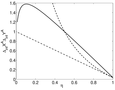
Figure 4: Effect of detector efficiencies $\eta_{A}$ and $\eta_{B}$ on the EPR paradox. Plot is $\mathcal{E}=\Delta_{inf}X^{A}\Delta_{inf}Y^{A}$ for a two-mode squeezed state with $r=2$: $\eta_{A}=\eta_{B}=\eta$ (solid line); fixed $\eta_{A}=1$ but varying $\eta=\eta_{B}$ (dashed line); fixed $\eta_{B}=1$ but varying $\eta=\eta_{A}$ (dashed-dotted line). The EPR paradox is sensitive to the losses $\eta_{B}$ of the “steering” system $B$, but insensitive to $\eta_{A}$, those of the “inferred” system $A$. No paradox is possible for $\eta_{B}\leq 0.5$, regardless of $\eta_{A}$, but a paradox is always possible with $\eta_{B}>0.5$, provided only $\eta_{A}>0$.

The effect of decoherence on entanglement is a topic of current interest (Eberly and Yu (2007)). Disentanglement in a finite time or ‘entanglement sudden death’ has been reported by Yu and Eberly (2004) for entangled qubits independently coupled to reservoirs that model an external environment. By comparison, the continuous variable entanglement is remarkably robust with respect to efficiency $\eta$. The death of EPR-entanglement at $\eta=0.5$ is a different story, and applies generally to Gaussian states that have symmetry with respect to phase and interchange of $A$ and $B$.

A fundamental difference between the continuous-variable EPR experiments and the experiments proposed by Bohm and Bell is the treatment of events in which no photon is detected. These null events give rise to loopholes in the photon-counting Bell experiments to date, as they require fair-sampling assumptions. In continuous-variable measurements, events where a photon is not detected simply correspond to the outcome of zero photon number $\widehat{a}_{\pm}^{\dagger}\widehat{a}_{\pm}$, so that $X_{\theta}^{A}=0$. These events are therefore automatically included in the measure $\mathcal{E}$ of EPR.

Our calculation based on the symmetric two-mode squeezed state reveals that efficiencies of $\eta>0.5$ are required to violate an EPR inequality. This is more easily achieved than the stringent efficiency criteria of Clauser and Shimony (1978) for a Bell inequality violation. It is also lower than the threshold for a spin EPR paradox (Section IV.B). To help matters further, homodyne detection is more efficient than single-photon detection. Recent experiments obtain overall efficiencies of $\eta>0.98$ for quadrature detection (Zhang et al. (2003a); Suzuki et al. (2006)), owing to the high efficiencies possible when operating silicon photo-diodes in a continuous mode.

VI EPR, entanglement and Bell criteria

In this Colloquium, we have understood a “demonstration of the EPR paradox” to be a procedure that closely follows the original EPR gedanken experiment. Most generally, the EPR paradox is demonstrated when one can confirm the inconsistency between local realism and the completeness of quantum mechanics, since this was the underlying EPR objective.

We point out in this Section that the inconsistency can be shown in more ways than one. There are many uncertainty relations or constraints placed on the statistics of a quantum state, and for each such relation there is an EPR criterion. This has been discussed for the case of entanglement by Gühne (2004), and for EPR by Cavalcanti and Reid (2007). It is thus possible to establish a whole set of criteria that are sufficient, but may not be necessary, to demonstrate an EPR paradox.

VI.1 “Steering”

The demonstration of an EPR paradox is a nice way to confirm the nonlocal effect of Schrödinger’s “steering”, a reduction of the wave-packet at a distance (Wiseman et al. (2007)).

An important simplifying aspect of the original EPR paradox is the asymmetric application of local realism to imply elements of reality for one system, the “inferred” or “steered” system. Within this constraint, we may generalize the EPR paradox, by applying local realism to all possible measurements, and testing for consistency of all the elements of reality for $A$ with a quantum state. One may apply (Cavalcanti et al. (2008)) the arguments of Section IV and the approach of Wiseman et al. (2007) to deduce the following condition for such consistency:

$$P(x_{\theta}^{A},x_{\phi}^{B})=\int_{\lambda}d\lambda P(\lambda)P_{Q}(x_{\theta}^{A}|\lambda)P(x_{\phi}^{B}|\lambda).$$ (32)

Here, notation is as for Eqs. (5) and (8), so that $P(x_{\theta}^{A},x_{\phi}^{B})$ is the joint probability for results $x_{\theta}^{A}$ and $x_{\phi}^{B}$ of measurements performed at $A$ and $B$ respectively, these measurements being parametrized by $\theta$ and $\phi$. The $\lambda$ is a discrete or continuous index, symbolizing hidden variable or quantum states, so that $P_{Q}(x_{\theta}^{A}|\lambda)$ and $P(x_{\phi}^{B}|\lambda)$ are both probabilities for outcomes given a fixed $\lambda$. Here as in Eq. (5), $P_{Q}^{A}(x_{\theta}^{A}|\lambda)=\langle x_{\theta}^{A}|\rho_{\lambda}|x_{\theta}^{A}\rangle$ for some quantum state $\rho_{\lambda}$, so that this probability satisfies all quantum uncertainty relations and constraints. There is no such restriction on $P^{B}(x_{\phi}^{B}|\lambda)$.

Eq. (32) has been derived recently by Wiseman et al. (2007), and its failure defined as a condition to demonstrate “steering”. These authors point out that Eq. (32) is the intermediate form of Eq. (5) to prove entanglement, and Eq. (8) used to prove failure of Bell’s local hidden variables. The failure of (32) may be considered an EPR paradox in a generalized sense. The EPR paradox as we define it, which simply considers a subset of measurements, is a special case of “steering”.

These authors also show that for quadrature phase amplitude measurements on bipartite Gaussian states, Eq. (32) fails when, and only when, the EPR criterion Eq. (23) (namely $\Delta_{inf}x\Delta_{inf}p<1$) is satisfied. This ensures that this EPR criterion is necessary and sufficient for the EPR paradox in this case.

VI.2 Symmetric EPR paradox

One can extend the EPR argument further, to consider not only the elements of reality inferred on $A$ by $B$, but those inferred on $B$ by $A$. It has been discussed by Reid (2004) that this symmetric application implies the existence of a set of shared “elements of reality”, which we designate by $\lambda$, and for which Eq. (8) holds. This can be seen by applying the reasoning of the previous section to derive sets of elements of reality $\lambda_{A/B}$ for each of $A$ and $B$ (respectively), that can be then shared to form a complete set $\left\{\lambda_{A},\lambda_{B}\right\}$. Explicitly, we can substitute $P(x_{\phi}^{B}|\lambda_{A})=\sum_{\lambda_{B}}P(x_{\phi}^{B}|\lambda_{B})P(\lambda_{B}|\lambda_{A})$ into (32) to get (8). Thus, EPR’s local realism can in principle be extrapolated to that of Bell’s, as defined by (8).

Where we violate the condition (5) for separability, to demonstrate entanglement, it is necessarily the case that the parameters $\lambda$ for each localized system cannot be represented as a quantum state. In this way, the demonstration of entanglement, for sufficient spatial separations, gives inconsistency of Bell’s local realism with completeness of quantum mechanics, and we provide an explicit link between entanglement and the EPR paradox.

VI.3 EPR as a special type of entanglement

While generalizations of the paradox have been presented, we propose to reserve the title “EPR paradox” for those experiments that minimally extend the original EPR argument, so that criteria given in Section IV are satisfied. It is useful to distinguish the entanglement that gives you an EPR paradox - we will define this to be “EPR-entanglement” - as a special form of entanglement. The EPR-entanglement is a measure of the ability of one observer, Bob, to gain information about another, Alice. This is a crucial and useful feature of many applications (Section X).

Entanglement itself is not enough to imply the strong correlation needed for an EPR paradox. As shown by Bowen et al. (2003a), where losses that cause mixing of a pure state are relevant, it is possible to confirm entanglement where an EPR paradox criterion cannot be satisfied (Section VII). That this is possible is understood when we realize that the EPR paradox criterion demands failure of Eq. (32), whereas entanglement requires only failure of the weaker condition Eq. (5). The observation of the EPR paradox is a stronger, more direct demonstration of the nonlocality of quantum mechanics than is entanglement; but requires greater experimental effort.

That an EPR paradox implies entanglement is most readily seen by noting that a separable (non-entangled) source, as given by Eq. (4), represents a local realistic description in which the localized systems $A$ and $B$ are described as quantum states $\widehat{\rho}_{\lambda}^{A/B}$. Recall, the EPR paradox is a situation where compatibility with local realism would imply the localized states not to be quantum states. We see then that a separable state cannot give an EPR paradox. Explicit proofs have been presented by Reid (2004), Mallon et al. (2008) and, for tripartite situations, Olsen et al. (2006).

The EPR criterion in the case of continuous variable measurements is written, from (20)

$$\mathcal{E}=\Delta\left(x-gx^{B}\right)\Delta\left(p+g^{\prime}p^{B}\right)<1\,\,.$$ (33)

where $g$ and $g^{\prime}$ are adjustable and arbitrary scaling parameters that would ideally minimise $\mathcal{E}$. The experimental confirmation of this inequality would give confirmation of quantum inseparability on demand, without postselection of data. This was first carried out experimentally by Ou et al. (1992).

Further criteria sufficient to prove entanglement for continuous variable measurements were presented by Duan et al. (2001) and Simon (2000), who adapted the PPT criterion of Peres (1996). These criteria were derived to imply inseparability (entanglement) rather than the EPR paradox itself and represent a less stringent requirement of correlation. The criterion of Duan et al. (2000), which gives entanglement when

$$D=[\Delta^{2}(x-x^{B})+\Delta^{2}(p+p^{B})]/4<1,$$ (34)

has been used extensively to experimentally confirm continuous variable entanglement (refer to references of Section XI). The criterion is both a necessary and sufficient measure of entanglement for the important practical case of bipartite symmetric Gaussian states.

We note we achieve the correlation needed for the EPR paradox, once $D<0.5$. This becomes transparent upon noticing that $xy\leq(x^{2}+y^{2})/2$, and so always $\Delta(x-x^{B})\Delta(p-p^{B})\leq 2D$. Thus, when we observe $D<0.5$, we know $\Delta(x-x^{B})\Delta(p+p^{B})\leq 1$, which is the EPR criterion (33) for $g=g^{\prime}=1$. The result also follows directly from (21), which gives, on putting $g=g^{\prime}=1$,

$$D=[\Delta^{2}(x-x^{B})+\Delta^{2}(p+p^{B})]/4<0.5$$ (35)

as sufficient to confirm the correlation of the EPR paradox. We note that this criterion, though sufficient, is not necessary for the EPR paradox. The EPR criterion (33) is more powerful, being necessary and sufficient for the case of quadrature phase measurements on Gaussian states, and can be used as a measure of the degree of EPR paradox. The usefulness of criterion (21) is that many experiments have reported data for it. From this we can infer an upper bound for the conditional variance product, since we know that $\mathcal{E}\leq 2D$.

Recent work explores measures of entanglement that might be useful for non-Gaussian and tri-partite states. Entanglement of formation (Bennett et al. (1996)) is a necessary and sufficient condition for all entangled states, and has been measured for symmetric Gaussian states, as outlined by Giedke et al. (2003) and performed by Josse et al. (2004) and Glöckl et al. (2004). There has been further work (Gühne (2004); Agarwal and Biswas (2005); Shchukin and Vogel (2005); Hillery and Zubairy (2006); Gühne and Lütkenhaus (2006)) although little that focuses directly on the EPR paradox. Inseparability and EPR criteria have been considered however for tripartite systems (Aoki et al. (2003); Jing et al. (2003); van Loock and Furusawa (2003); Bradley et al. (2005); Villar et al. (2006)).

VI.4 EPR and Bell’s nonlocality

A violation of a Bell inequality gives a stronger conclusion than can be drawn from a demonstration of the EPR paradox alone, but is more difficult to achieve experimentally. The predictions of quantum mechanics and local hidden variable theories are shown to be incompatible in Bell’s work. This is not shown by the EPR paradox.

The continuous variable experiments discussed in Sections VI and VII are excellent examples of this difference. It is well-known (Bell (1988)) that a local hidden variable theory, derived from the Wigner function, exists to explain all outcomes of these continuous variable EPR measurements. The Wigner function c-numbers take the role of position and momentum hidden variables. For these Gaussian squeezed states the Wigner function is positive and gives the probability distribution for the hidden variables. Hence, for this type of state, measuring $x$ and $p$ will not violate a Bell inequality.

If the states generated in these entangled continuous variable experiments are sufficiently pure, quantum mechanics predicts that it is possible to demonstrate Bell’s nonlocality for other measurements (Grangier et al. (1988); Oliver and Stroud (1989); Praxmeyer et al. (2005)). This is a general result for all entangled pure states, and thus also for EPR states (Gisin and Peres (1992)). The violation of Bell’s inequalities for continuous variable (position/ momentum) measurements has been predicted for only a few states, either using binned variables (Leonhardt and Vaccaro (1995); Gilchrist et al. (1998); Yurke et al. (1999); Munro and Milburn (1998); Wenger et al. (2003)) or directly using continuous multipartite moments (Cavalcanti et al. (2007b)). An interesting question is how the degree of inherent EPR paradox, as measured by the conditional variances of Eq. (33), relates quantitatively to the Bell inequality violation available. This has been explored in part, for the Bohm EPR paradox, by Filip et al. (2004).

It has been shown by Werner (1989) that for mixed states, entanglement does not guarantee that Bell’s local hidden variables will fail for some set of measurements. One can have entanglement (inseparability) without a failure of local realism. The same holds for EPR-entanglement. For two-qubit Werner states, violation of Bell inequalities demands greater purity ($p_{W}>0.66$ (Acín et al. (2006)) than does the EPR-Bohm paradox, which can be realized for $p_{W}>0.62$ (Section IV).

VII Continuous-wave EPR experiments

VII.1 Parametric oscillator experiments

The first continuous variable test of the EPR paradox was performed by Ou et al. (1992). These optically-based EPR experiments use local-oscillator measurements with high efficiency photo-diodes, giving overall efficiencies of more than $80\%$, even allowing for optical losses (Ou et al. (1992b); Grosshans et al. (2003)). This is well above the $50\%$ efficiency threshold required for EPR.

Rather than interrogating the position and momentum of particles as initially proposed by Einstein, Podolsky, and Rosen, analogous but more convenient variables were used — the amplitude and phase quadratures of optical fields, as described in Section V. The EPR correlated fields in the experiment of Ou et al. (1992) (Fig. 5) were generated using a sub-threshold nondegenerate type II intra-cavity optical parametric oscillator in a manner proposed by Reid and Drummond (Reid and Drummond (1988); Reid (1989); Drummond and Reid (1990); Dechoum et al. (2004)). of a type II $\chi^{(2)}$ non-linear process in which pump photons at some frequency $\Omega_{\textrm{pump}}$ are converted to pairs of correlated signal and idler photons with orthogonal polarizations and frequencies satisfying $\Omega_{\textrm{signal}}+\Omega_{\textrm{idler}}=\Omega_{\textrm{pump}}$. As discussed in Section V, these experiments utilize a spectral filtering technique to select an output temporal mode, with a detected duration $\Delta t$ that is typically of order $1\mu s$ or more. This issue, combined with the restricted detector separations used to date, means that a true, causally separated EPR experiment is yet to be carried out, although this is certainly not impossible. In all these experiments the entangled beams are separated and propagate into different directions, so the only issue is the duration of the measurement. This proposal uses cavities which are single-mode in the vicinity of each of the resonant frequencies, so modes must be spatially separated after output from the cavity. Another possibility is to use multiple transverse modes together with type I (degenerate) phase-matching, as proposed by Castelli and Lugiato (1997); Olsen and Drummond (2005).

For an oscillator below threshold and at resonance, we are interested in traveling wave modes of the output fields at frequencies $\omega_{A}$ and $\omega_{B}$. These are in an approximate two-mode squeezed state, with the quadrature operators as given by Eq. (26). In these steady-state, continuous-wave experiments, however, the squeezing parameter $r$ is time-independent, and given by the input-output parametric gain $G$, such that $G=e^{2r}$. Apart from the essential output mirror coupling, losses like absorption in the nonlinear medium cause non-ideal behavior and reduce correlation as described in the Section V.

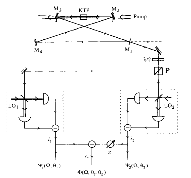
Figure 5: The original EPR parametric downconversion experiment using an intracavity nonlinear crystal and homodyne detection, following the procedure depicted in Fig. 3. Figure reprinted from Ou et al. (1992), with permission.

Restricting ourselves to the lossless, ideal case for the moment, we see that as the gain of the process approaches infinity ($G\rightarrow\infty$) the quadrature operators of beams $a$ and $b$ are correlated so that:

$$\left\langle\left(\hat{x}^{A}-\hat{x}^{B}\right)^{2}\right\rangle \rightarrow 0$$

$$\left\langle\left(\widehat{Y}^{A}+\widehat{Y}^{B}\right)^{2}\right\rangle \rightarrow 0.$$ (36)

Therefore in this limit an amplitude quadrature measurement on beam $a$ would provide an exact prediction of the amplitude quadrature of beam $b$; and similarly a phase quadrature measurement on beam $a$ would provide an exact prediction of the phase quadrature of beam $b$. This is a demonstration of the EPR paradox in the manner proposed in Einstein et al. (1935). An alternative scheme is to use two independently squeezed modes $\widehat{a}_{1},\widehat{a}_{2}$, which are combined at a $50\%$ beam-splitter so that the two outputs are $\widehat{a}_{A,B}=\left[\widehat{a}_{1}\pm i\widehat{a}_{2}\right]/\sqrt{2}$. This leads to the same results as Eq. (26), and can be implemented if only type-I (degenerate) down-conversion is available experimentally.

VII.2 Experimental Results

In reality, we are restricted to the physically achievable case where losses do exist, and the high non-linearities required for extremely high gains are difficult to obtain. Even so, with some work at minimizing losses and enhancing the non-linearity, it is possible to observe the EPR paradox. Since, in general, the non-linear process is extremely weak, one of the primary goals of an experimentalist is to find methods to enhance it. In the experiment of Ou et al. (1992) the enhancement was achieved by placing the non-linear medium inside resonant cavities for each of the pump, signal, and idler fields. The pump field at 0.54 $\mu$m was generated by an intracavity frequency doubled Nd:YAP laser, and the non-linear medium was a type II non-critically phase matched KTP crystal. The signal and idler fields produced by the experiment were analyzed in a pair of homodyne detectors. By varying the phase of a local oscillator, the detectors could measure either the amplitude or the phase quadrature of the field under interrogation, as described in Section V. Strong correlations were observed between the output photocurrents both for joint amplitude quadrature measurement, and for joint phase quadrature measurement. To characterize whether their experiment demonstrated the EPR paradox, and by how much, Ou et al. (1992) used the EPR paradox criterion given in Eq. (23) and Eq. (20). They observed a value of $\mathcal{E}^{2}=0.70<1$, thereby performing the first direct experimental test of the EPR paradox, and hence demonstrating entanglement (albeit without causal separation).

The EPR paradox was then further tested by Silberhorn et al. (2001); Schori et al. (2002); Bowen et al. (2003a); Bowen et al. (2004). Most tests were performed using optical parametric oscillators. Both type I (Bowen et al. (2003a); Bowen et al. (2004)) and type II (Ou et al. (1992)) optical parametric processes, as well as various non-linear media have been utilized. Type I processes produce only a single squeezed field, rather than a two mode squeezed field, so that double the resources are required in order that the two combined beams are EPR correlated. However, such systems have significant benefits in terms of stability and controllability. Improvements have been made not only in the strength and stability of the interaction, but in the frequency tunability of the output fields (Schori et al. (2002)), and in overall efficiency. The optimum level of EPR-paradox achieved to date was by Bowen et al. (2003a) using a pair of type I optical parametric oscillators. Each optical parametric oscillator consisted of a hemilithic MgO:LiNbO₃ non-linear crystal and an output coupler. MgO:LiNbO₃ has the advantage over other non-linear crystals of exhibiting very low levels of pump induced absorption at the signal and idler wavelengths (Furukawa et al. (2001). Furthermore, the design, involving only one intracavity surface, minimized other sources of losses, resulting in a highly efficient process. The pump field for each optical parametric amplifier was produced by frequency doubling an Nd:YAG laser to 532 nm. Each optical parametric amplifier produced a single squeezed output field at 1064 nm, with 4.1 dB of observed squeezing. These squeezed fields were interfered on a 50/50 beam splitter, producing a two-mode squeezed state as described in Eq. (26). A degree of EPR paradox $\mathcal{E}^{2}=0.58$ was achieved. These results were verified by calibrating the loss. The losses were experimentally varied and the results compared with theory (Section VI), as shown in Fig. 6. This can be improved further, as up to $9$ dB single-mode squeezing is now possible (Takeno et al. (2007). These experiments are largely limited by technical issues like detector mode-matching and control of the optical phase-shifts, which can cause unwanted mixing of squeezed and unsqueezed quadratures.

Another technique is bright-beam entanglement above threshold, proposed by Reid and Drummond (1988, 1989) and Castelli and Lugiato (1997). This was achieved recently in parametric amplifiers (Villar et al. (2005); Jing et al. (2006); Su et al. (2006); Villar et al. (2007))) and eliminates the need for an external local oscillator. Dual-beam second-harmonic generation can also theoretically produce EPR correlations (Lim and Saffman (2006)). We note that the measure $\mathcal{E}^{2}=0.58$ is to the best of our knowledge the lowest recorded result where there has been a direct measurement of an EPR paradox. A value for $\mathcal{E}^{2}$ can be often be inferred from other data, either with assumptions about symmetries (Laurat et al. (2005)), or as an upper bound, from a measurement of the Duan et al. (2000) inseparability $D$, since we know $\mathcal{E}\leq 2D$ (Eq. (21, Section VI). Such inferred values imply measures of EPR paradox as low as $\mathcal{E}^{2}=0.42$ (Laurat et al. (2005), Section XI).

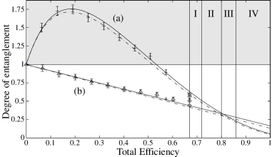
Figure 6: Graph of (a) the EPR-paradox measure $\mathcal{E}^{2}$ (Eqs. (23), (20), (33)) and (b) Duan et al. (normalized) entanglement measure $D$ (Eq. (34)) vs. total efficiency $\eta.$ The dashed lines are theoretical predictions for $\mathcal{E}^{2}$ and $\mathcal{D}$. The points are experimental data with error bars. It is more difficult to satisfy the EPR paradox than to demonstrate entanglement. Figure reprinted from Bowen et al. (2003a), with permission.

There has also been interest in the EPR-entanglement that can be achieved with other variables. Bowen et al. (2002b) obtained $\mathcal{E}^{2}=0.72$ for the EPR paradox for Stokes operators describing the field polarization. The EPR paradox was tested for the actual position and momentum of single photons (Fedorov et al. (2004, 2006); Guo and Guo (2006)) in an important development by Howell et al. (2004) to realize an experiment more in direct analogy with original EPR. Here, however, the exceptional value $\mathcal{E}^{2}=0.01$ was achieved using conditional data, where detection events are only considered if two emitted photons are simultaneously detected. The results are thus not directly applicable to the a priori EPR paradox. The entanglement of momentum and position, as described in the original EPR paradox, and proposed by Castelli and Lugiato (1997) andLugiato et al. (1997) has been achieved using spatially entangled laser beams (Wagner et al. (2008); Boyer et al. (2008)).

VIII Pulsed EPR experiments

In the previous section we mentioned that one of the goals of an experimentalist who aims at generating efficient entanglement is to devise techniques by which the effective nonlinearity can be enhanced. One solution is to place the nonlinear medium inside a cavity, as discussed above, and another one, which will be discussed in this section, is to use high power pump laser pulses. By using such a source the effective interaction length can be dramatically shortened. The high finesse cavity conditions can be relaxed or for extreme high peak power pulses, the use of a cavity can be completely avoided. In fact a single pass through either a highly nonlinear $\chi^{(2)}$ medium (Slusher et al. (1987); Aytür and Kumar (1990); Hirano and Matsuoka (1990); Smithey et al. (1992)), or through a relatively short piece of standard glass fiber with a $\chi^{(3)}$ nonlinear coefficient (Rosenbluh and Shelby (1991); Bergman and Haus (1991)), suffices to generate quantum squeezing, which in turn can lead to entanglement.

The limitations imposed by the cavity linewidth in the CW experiment, such as production of entanglement in a narrow frequency band (e.g. generation of "slow" entanglement), are circumvented when employing a single pass pulsed configuration. The frequency bandwidth of the quantum effects is then limited only by the phase matching bandwidth as well as by the bandwidth of the nonlinearity, both of which can be quite large, e.g. on the order of some THz (Sizmann and Leuchs (1999)). Broadband entanglement is of particular importance for the field of quantum information science, where for example it allows for fast communication of quantum states by means of quantum teleportation (Section X). This may also allow truly causal EPR experiments, which are yet to be carried out.

VIII.1 Optical fiber experiment

The first experimental realization of pulsed EPR entanglement, shown in Fig. 7 was based on the approach of mixing two squeezed beams on a 50/50 beam splitter as outlined above for CW light. In this experiment the two squeezed beams were generated by exploiting the Kerr nonlinearity of silica fibers (Carter et al. (1987); Rosenbluh and Shelby (1991)) along two orthogonal polarization axes of the same polarization maintaining fiber (Silberhorn et al. (2001)). More precisely, the fiber was placed inside a Sagnac interferometer to produce two amplitude squeezed beams, which subsequently interfered at a bulk 50/50 beam splitter (or fiber beam splitter as in Nandan et al. (2006)) to generate two spatially separated EPR modes possessing quantum correlations between the amplitude quadratures and the phase quadratures.

The Kerr effect is a $\chi^{(3)}$ non-linear process and is largely equivalent to an intensity dependent refractive index. It corresponds to a four photon mixing process where two degenerate pump photons at frequency $\Omega$ are converted into pairs of photons (signal and idler photons) also at frequency $\Omega$. Due to the full degeneracy of the four-photon process, phase matching is naturally satisfied and no external control is needed. Apart from this, optical parametric amplification and four wave mixing are very similar (Milburn et al. (1987)). The nonlinear susceptibility for the Kerr effect, $\chi^{(3)}$, is very small compared to the one for optical parametric amplification, $\chi^{(2)}$. However, as noted above, the effect is substantially enhanced by using high peak power pulses as well as fibers resulting in strong power confinement over the entire length of the fiber crystal. In the experiment of Silberhorn et al. (2001) a 16 m long polarization maintaining fiber was used, the pulse duration was 150 fs, the repetition rate was 163 MHz and the mean power was approximately 110 pJ. The wavelength was the telecommunication wavelength of 1.55$\mu$m at which the optical losses in glass are very small (0.1 dB/km) and thus almost negligible for 16 m of fiber. Furthermore, at this wavelength the pulses experience negative dispersion which together with the Kerr effect enable soliton formation at a certain threshold pulse energy, thereby ensuring a constant peak power level of the pulses along the fiber.

The formation of solitons inside a dispersive medium is due to the cancellation of two opposing effects - dispersion and the Kerr effect. However, this is a classical argument and thus does not hold true in the quantum regime. Instead, an initial coherent state is known to change during propagation in a nonlinear medium, leading to the formation of a squeezed state (Kitagawa and Yamamoto (1986); Carter et al. (1987); Drummond et al. (1993)). Both squeezed and entangled state solitons have been generated in this way.

When obtaining entanglement via Kerr-induced squeezing, as opposed to the realizations with few photons described in the previous section, the beams involved are very bright. This fact renders the verification procedure of proving EPR entanglement somewhat more difficult since standard homodyne detectors cannot be used. We note that the conjugate quadratures under interrogation of the two beams need not be detected directly; it suffices to construct a proper linear combination of the quadratures, e.g. $\hat{x}^{A}+\hat{x}^{B}$ and $\widehat{Y}^{A}-\widehat{Y}^{B}$. In Silberhorn et al. (2001) a 50/50 beam splitter (on which the two supposedly entangled beams were interfering) followed by direct detection of the output beams and electronic subtraction of the generated photocurrents was used to construct the appropriate phase quadrature combination demonstrating the phase quadrature correlations. Direct detection of the EPR beam was employed to measure the amplitude quadrature correlations (see also references Glöckl et al. (2004, 2006)). Based on these measurements a degree of non-separability of $D=0.40$ was demonstrated (without correcting for detection losses). The symmetry of the entangled beams allowed one to infer from this number the degree of EPR violation, which was found to be $\mathcal{E}^{2}=0.64\pm 0.08$.

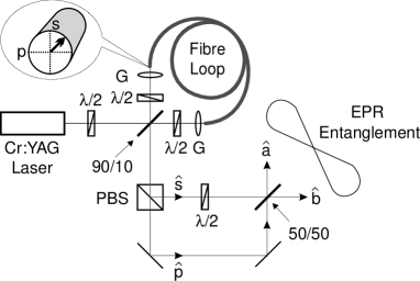
Figure 7: The original demonstration of pulsed EPR entanglement. The soliton experiment uses orthogonal polarization modes in a fiber Sagnac interferometer and a Mach-Zehnder interferometer for fiber-birefringence compensation. Notation: $\lambda/2$ means half-wave plate; $G$ is a gradient index len; $50/50$ means beam splitter of 50% reflectivity; $\hat{s}$ and $\hat{p}$ are two amplitude squeezed beams from the respective polarization states; $\hat{a}$ and $\hat{b}$ are EPR entangled beams. Figure reprinted from Silberhorn et al. (2001) with permision.

The degree of entanglement as well as the purity of the EPR state generated in this experiment were partly limited by an effect referred to as guided acoustic wave Brillouin scattering (GAWBS) (Shelby et al. (1985)), which occurs unavoidably in standard fibers. This process manifests itself through thermally excited phase noise resonances ranging in frequency from a few megahertz up to some gigahertz and with intensities that scales linearly with the pump power and the fiber length. The noise is reduced by cooling the fiber (Shelby et al. (1986)), using intense pulses (Shelby et al. (1990)) or by interference of two consecutive pulses which have acquired identical phase noise during propagation (Shirasaki and Haus (1992)). Recently it was suggested that the use of certain photonic crystal fibers can reduce GAWBS (Elser et al. (2006)). Stokes parameter entanglement has been generated exploiting the Kerr effect in fibers using a pulsed pump source (Glöckl et al. (2003)). A recent experiment (Huntington et al. (2005)) has shown that adjacent sideband modes (with respect to the optical carrier) of a single squeezed beam possess quadrature entanglement. However in both experiments the EPR inequality was not violated, partly due to the lack of quantum correlations and partly due to the extreme degree of excess noise produced from the above mentioned scattering effects.

VIII.2 Parametric amplifier experiment

An alternative approach, which does not involve GAWBS, is the use of pulsed down-conversion. Here one can either combine two squeezed pulses from a degenerate down-conversion process, or else directly generate correlated pulses using non-degenerate down-conversion. In these experiments, the main limitations are dispersion (Raymer et al. (1991)) and absorption in the nonlinear medium. Wenger et al. (2005) produced pulsed EPR beams, using a traveling-wave optical parametric amplifier pumped at 423 nm by a frequency doubled pulsed Ti:Sapphire laser beam. Due to the high peak powers of the frequency doubled pulses as well as the particular choice of a highly non-linear optical material (KNBO₃), the use of a cavity was circumvented despite the fact that a very thin (100 $\mu m$) crystal was employed. A thin crystal was chosen in order to enable broadband phase matching, thus avoiding group-velocity mismatch. The output of the parametric amplifier was then a pulsed two-mode squeezed vacuum state with a pulse duration of 150 fs and a repetition rate of 780 kHz.

In contrast to the NOPA used by Ou et al. (1992), which was non-degenerate in polarization, the process used by Wenger et al. was driven in a spatially non-degenerate configuration so the signal and idler beams were emitted in two different directions. In this experiment the entanglement was witnessed by mixing the two EPR beams with a relative phase shift of $\phi$ at a 50/50 beam splitter and then monitoring one output using a homodyne detector. Setting $\phi=0$ and $\phi=\pi$, the combinations $\hat{x}^{A}+\hat{x}^{B}$ and $\widehat{Y}^{A}-\widehat{Y}^{B}$ were constructed. They measured a non-separability of $D=0.7$ (without correcting for detector losses). Furthermore the noise of the individual EPR beams were measured and all entries of the covariance matrix were estimated (assuming no inter- and intra-correlations).

Without correcting for detector inefficiencies we deduce that the EPR paradox was not demonstrated in this experiment since the product of the conditional variances amounts to $\mathcal{E}^{2}=1.06$. However, by correcting for detector losses as done in the paper by Wenger et al., the EPR paradox was indeed achieved since in this case the EPR-product is $\mathcal{E}^{2}=0.83$, although causal separation was not demonstrated. A degenerate waveguide technique, together with a beam-splitter, was recently used to demonstrate pulsed entanglement using a traveling wave OPA (Zhang et al. (2007)).

A distinct difference between the two pulsed EPR experiments, apart from the non-linearity used, is the method by which the data processing was carried out. In the experiment by Silberhorn et al. (2001) , measurements were performed in the frequency domain similar to the previously discussed CW experiments: The quantum noise properties were characterized at a specific Fourier component within a narrow frequency band, typically in the range 100-300 kHz. The frequency bandwidth of the detection system was too small to resolve successive pulses, which arrived at the detector with a frequency of 163 MHz. In the experiment of Wenger et al., however, the repetition rate was much lower (780kHz), which facilitated the detection stage and consequently allowed for temporally-resolved measurements around DC (Smithey et al. (1992, 1993)).

IX Spin EPR and atoms

Experimental realizations of the paradox with massive particles are important, both due to their closeness in spirit with the original EPR proposal, and because such massive entities could reasonably be considered more closely bound to the concept of local realism than fields. To date, experimental tests of the EPR paradox with massive particles have been limited to situations of small spatial separation. However, the technology required to generate, manipulate, and interrogate non-classical states of massive systems has undergone rapid development over the past decade. These often involve spin-equivalent versions of the EPR paradox with spin quantum numbers much larger than one half. A spin-one (four-particle) Bell inequality violation of a type predicted by Drummond (1983) was observed experimentally by Howell et al. (2002). Criteria for observing a spin EPR paradox and the experimental test of Bowen et al. (2002a) have been discussed in Section IV.B.

Many theoretical proposals and experimental techniques to entangle pairs of atoms and atomic ensembles have been developed (Cirac et al. (1997)). The core technologies involved range from single neutral atoms trapped in high-$Q$ optical microresonators and manipulated with optical pulses (Kimble (1998); McKeever et al. (2003)), to multiple ions trapped in magnetic traps with interaction achieved through vibrational modes, to optically dense ensembles of atoms (Polzik (1999); Julsgaard et al. (2001, 2004); Kuzmich et al. (2000)).

Future experiments on ultra-cold atoms may involve direct entanglement of the atomic position. Possible experimental systems were recently analyzed by Fedorov et al. (2006), for pairs of massive or massless particles. Another approach for EPR measurements is to use correlated atom-laser beams generated from molecular dissociation (Kheruntsyan et al. (2005)). This proposal involves macroscopic numbers of massive particles, together with superpositions of different spatial mass-distributions. Entanglement of this type therefore could test the unification of quantum theory with gravity.

Here we focus on experiments based on atomic ensembles, which have shown the most promise for tests of the EPR paradox. In these, a weak atom-light interaction is used to generate a coherent excitation of the spin state of a large number of atoms within the ensemble.Through appropriate optical manipulation, both squeezing and entanglement of this collective macroscopic spin state have been demonstrated (Geremia et al. (2004); Kuzmich et al. (1997, 2000); Hald et al. (1999)), as well as entanglement of spatially separated atomic ensembles (Julsgaard et al. (2004); Chou et al. (2005); Chaneliére et al. (2005); Matsukevich et al. (2006)).

Decoherence is a critical factor which limits the ability to generate squeezing and entanglement in atomic systems. One might expect that since spin-squeezed and entangled atomic ensembles contain a large number $N$ of atoms, the decoherence rate of such systems would scale as $N\gamma$ where $\gamma$ is the single atom decay rate. Indeed, this is the case for other multi-particle entangled states such as Greenberger-Horne-Zeilinger entanglement (Greenberger et al. (1989)). However, a critical feature of these collective spin states is that excitation due to interaction with light is distributed symmetrically amongst all of the atoms. This has the consequence that the system is robust to decay (or loss) of single atoms. Consequently, the decoherence rate has no dependence on $N$ and is equal to the single photon decay rate $\gamma$ (Lukin (2003)). Several experimental techniques have been developed to further reduce the decoherence rate. These include the use of buffer gases (Phillips et al. (2001)) and paraffin coatings (Julsgaard et al. (2001)) in room temperature vapor cells to respectively minimize collisions between atoms and the effect of wall collisions; and the use of cold atoms in magneto-optic traps (Geremia et al. (2004)). These techniques have lead to long decoherence times of the order of 1 ms for the collective spin states.

IX.1 Transfer of optical entanglement to atomic ensembles

The work of Polzik (1999) showed that the optical entanglement generated by a parametric oscillator, as described in Section VII could be transferred to the collective spin state of a pair of distant atomic ensembles. This research built on earlier work focusing on the transfer of optical squeezing to atomic spin states (Kuzmich et al. (1997)). In both cases, however, at least 50% loss was introduced due to spontaneous emission. As discussed in Section V, the EPR paradox cannot be tested when symmetric losses that exceed $50$%. Therefore, the proposal of Polzik (1999) is not immediately suitable for tests of the EPR paradox. Extensions of this work have shown that by placing the atomic ensemble within an optical resonator, the quantum state transfer can be enhanced so that tests of the EPR paradox should be possible (Dantan et al. (2003); Vernac et al. (2001)).

The first experimental demonstration of quantum state transfer from the polarization state of an optical field to the collective spin state of an atomic ensemble was performed by Hald et al. (1999). They demonstrated transfer of as much as -0.13 dB of squeezing to an ensemble of $10^{9}$ cold atoms in a magneto-optic trap. The extension of these results to pairs of spatially separated entangled ensembles has yet to be performed experimentally.

IX.2 Conditional atom ensemble entanglement

The other approach to experimental demonstration of collective spin entanglement in atomic ensembles is to rely on conditioning measurements to prepare the state (Julsgaard et al. (2004); Chou et al. (2005)). This approach has the advantage of not requiring any non-classical optical resources. Kuzmich et al. (2000) performed an experiment that was based on a continuous quantum non-demolition (QND) measurement of the $z$ spin projection of a room temperature ensemble of spin-polarized Cesium atoms in a paraffin-coated glass cell and demonstrated 5.2 dB of collective spin squeezing. A subsequent experiment along theses lines by Geremia et al. (2004) utilized control techniques to further enhance the generation of QND based collective spin squeezing. The definition of collective spin in extended atomic systems of this type is discussed in Drummond and Raymer (1991).

In a major advance, collective spin entanglement was generated by Julsgaard et al. (2001) using techniques similar to the QND measurements above. They interacted a pulse of light with two spatially separated spin-polarized atomic ensembles in paraffin-coated glass cells, and performed a nonlocal Bell measurement on the collective spin through detection of the transmitted pulse. This conditioned the state of the atomic ensembles into a collective entangled state of the type required to test the EPR paradox. They report that if utilised in a unity gain coherent state teleportation experiment, this atomic entanglement could allow a fidelity as high as 0.55. This corresponds to an inseparability value of D = 0.82, which is well below 1 (indicating entanglement), but is not sufficient for a direct test of the EPR paradox.

Recently, techniques to condition the spin state of atomic ensembles have been developed based on the detection of stimulated Raman scattering. These techniques have significant potential for quantum information networks (Duan et al. (2001)) and are also capable of generating a collective entangled state of the form required to test the EPR paradox. The experiment by Kuzmich et al. (2003) demonstrated non-classical correlations between pairs of time-separated photons emitted from a Cs ensemble in a magneto-optical trap. Through the detection of the second photon the atomic ensemble was conditioned into a non-classical state. The principle of the experiment by van der Wal et al. (2003) was the same. However, a Rb vapor cell with buffer gas was used, and field quadratures were detected rather than single photons. This experiment demonstrated joint-squeezing of the output fields from the ensemble, implying the presence of collective spin squeezing within the ensemble. Entanglement between two spatially separate ensembles has now been demonstrated based on the same principles (Chou et al. (2005); Matsukevich et al. (2006)).

X Application of EPR entanglement

Entanglement is a central resource in many quantum information protocols. A review of the continuous variable quantum information protocols has been given by Braunstein and van Loock (2005). In this section, we focus on three continuous-variable quantum information protocols that utilize shared EPR entanglement between two parties. They are entanglement-based quantum key distribution, quantum teleportation and entanglement swapping. We discuss the relevance of the EPR paradox in relation to its use as a figure of merit for characterizing the efficacy of each of these protocols.

X.1 Entanglement-based quantum key-distribution

In quantum key distribution (QKD), a sender, Alice, wants to communicate with a receiver, Bob, in secrecy. They achieve this by first cooperatively finding a method to generate a secret key that is uniquely shared between the two of them. Once this key is successfully generated and shared, messages can be encrypted using a “one-time-pad” algorithm and communication between them will be absolutely secure. Figure 3 shows that the EPR paradox can be demonstrated when Alice and Bob get together to perform conditional variance measurements of the quadrature amplitudes of a pair of entangled beams. The product of the conditional variances of both quadrature amplitudes gives the degree of EPR entanglement. Since EPR entangled beams cannot be cloned, it has been proposed by Reid (2000) and Silberhorn et al. (2002) that the sharing of EPR entanglement between two parties can be used for QKD.

In order to use the EPR entanglement for QKD, we assume that the entanglement generation is performed by Alice. Alice keeps one of the entangled beams and transmits the other to Bob. It is therefore reasonable to assume that Alice’s measurements on her beam has negligible loss by setting $\eta_{A}=1$ whilst Bob’s measurements are lossy due to the long distance transmission of entanglement with $\eta_{B}<1$. With Alice and Bob both randomly switching their quadrature measurement between amplitude ($X^{A}$ for Alice and $X^{B}$ for Bob) and phase ($Y^{A}$ for Alice and $Y^{B}$ for Bob), the secret key for the cryptographic communication is obtained from the quantum fluctuations of the EPR entanglement when there is an agreement in their chosen quadrature.

Since the results of measurements between Alice and Bob are never perfectly identical, Alice and Bob are required to reconcile the results of their measurements. Conventionally, it was assumed that Bob is required to guess Alice’s measured values. The net information rate for QKD, as suggested by Csiszár and Körner (1978), is given by

$$\Delta I=\frac{1}{2}\log_{2}\left(\frac{V_{A|E}^{X}V_{A|E}^{Y}}{V_{A|B}^{X}V_{A|B}^{Y}}\right)$$ (37)

where $V_{A|B}^{X}=\Delta_{inf}^{2}X^{A}$ and $V_{A|B}^{Y}=\Delta_{inf}^{2}Y^{A}$ are the conditional variances defined in Section IV.3 for inferences made about $A$ from $B$, and where $V_{A|E}^{X,Y}$ is calculated by assuming that an eavesdropper Eve has access to all of the quantum correlations resulting from transmission losses. When the net information rate is positive, $\Delta I>0$, a secret key can be generated between Alice and Bob. The conditional variance product $V_{A|B}=\Delta_{inf}^{2}X^{A}\Delta_{inf}^{2}Y^{A}$ can be written:

$$V_{A|B}=\left[V_{A}^{X}-\frac{\left|\left\langle\hat{x}^{B},\hat{x}^{A}\right\rangle\right|^{2}}{V_{B}^{X}}\right]\left[V_{A}^{Y}-\frac{\left|\left\langle\widehat{Y}^{B},\widehat{Y}^{A}\right\rangle\right|^{2}}{V_{B}^{Y}}\right]$$ (38)

Here we define $V_{A,B}^{X}=\Delta^{2}X^{A,B}$, and $V_{A,B}^{Y}=\Delta^{2}Y^{A,B}$. We note from Fig. 4 that $V_{A|B}>1$ for $\eta_{B}<0.5$. This suggests that Alice and Bob can no longer share EPR entanglement for larger than 3 dB transmission loss. This loss limit is referred to as the 3 dB limit for QKD.

If on the other hand, Alice was to infer Bob’s measured results, the relevant EPR measure and net information rate are respectively given by

$$V_{B|A} = \left[V_{A}^{X}-\frac{\left|\left\langle\hat{x}^{B},\hat{x}^{A}\right\rangle\right|^{2}}{V_{A}^{X}}\right]\left[V_{B}^{Y}-\frac{\left|\left\langle\widehat{Y}^{B},\widehat{Y}^{A}\right\rangle\right|^{2}}{V_{A}^{Y}}\right]$$

$$\Delta I = \frac{1}{2}\log_{2}\left(\frac{V_{B|E}^{X}V_{B|E}^{Y}}{V_{B|A}^{X}V_{B|A}^{Y}}\right)$$ (39)

Fig. 4 suggests that it is possible to have $V_{B|A}\leq 1$ and $\Delta I>0$ for all values of $0<\eta_{B}<1$. Entanglement can thus exist over long distances and the 3 dB limit for entanglement-based QKD can be surpassed.

The advantage gained by reversing the inference, known as reverse reconciliation, was first recognized by Grosshans et al. (2003). It can be simply understood as follows. When Bob and Eve both attempt to infer the information Alice sent using their respective measurements, a greater than $50\%$ loss where $\eta_{B}<0.5$ will give Eve an irrecoverable information advantage over Bob since one has to assume that Eve somehow has access to more than 50% of the information. In reverse reconciliation, Alice and Eve will both attempt to infer Bob’s results. Since Alice’s entanglement is assumed to be lossless ($\eta_{A}=1$), she maintains her information advantage relative to Eve, who only has partial information that is at most proportional to transmission losses.

X.2 Quantum Teleportation and Entanglement Swapping

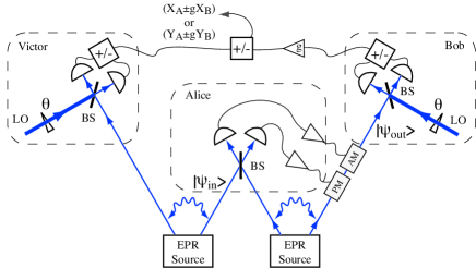
Figure 8: (Color online) Schematic of quantum teleportation and entanglement swapping. In teleportation, Alice and Bob share a pair of entangled beams. $|\psi_{{\rm in}}\rangle$ is the input state Alice teleports to Bob. The use of electro-optic feedforward on both the amplitude and phase quadrature on Bob’s entangled beam produces an output state $|\psi_{{\rm out}}\rangle$ which he measures using optical homodyne detection, as in Fig. 3. In entanglement swapping, Alice and Victor also share a pair of entangled beams. Alice uses her share of this pair as the input state $|\psi_{{\rm in}}\rangle$. The teleportation protocol is again performed. Victor verifies the efficacy of entanglement swapping using conditional variance measurements of his entangled beam with Bob’s teleportation output beam. The elements are: beam splitters BS, local oscillator LO, phase shift $\theta$, difference/ sum currents $+/-$. Semicircles are photodiodes, while triangles show electronic gain.

Quantum teleportation is a three stage protocol that enables a sender, Alice, to transmit a quantum state to a receiver, Bob, without a direct quantum channel. Fig. 8 gives the schematic of the protocol. Alice first makes simultaneous measurements of a pair of conjugate observables of an unknown quantum state, $|\psi\rangle$, by interfering the unknown quantum state with one of the entangled beam pairs she shares with Bob. She then transmits both her measured results to Bob using two classical channels. Using the other entangled beam, Bob reconstructs the quantum state by manipulation of the other entangled beam, using the classical information obtained from Alice. In an ideal situation, the output state of Bob will be an exact replica of the unknown input state sent by Alice. This form of remote communication of quantum information using only entanglement and classical information was proposed by Bennett et al. (1993) for discrete variables. A year later, Vaidman (1994) extended this idea to allow for continuous-variable systems, such as the teleportation of position and momentum of a particle or the quadrature amplitudes of a laser beam. Further work on continuous-variable quantum teleportation by Braunstein and Kimble (1998) and Ralph and Lam (1998) shows that quantum teleportation can indeed be demonstrated using finite squeezing and entanglement.

For realistic experimental demonstration of continuous-variable quantum teleportation, the output state cannot be identical to the teleporter input because of the finite quantum correlations available in experimentally produced squeezing and entanglement. A well accepted measure of teleportation efficacy is the overlap of the wavefunction of the output state with the original input state. The teleportation fidelity is given by ${\cal F}=\langle\psi_{{\rm in}}|\widehat{\rho}_{{\rm out}}|\psi_{{\rm in}}\rangle$ where $\widehat{\rho}_{{\rm out}}$ is the density operator of the output state. Ideally, quantum teleportation can give a fidelity of unity. For a Gaussian distribution of coherent states, with mean photon number $\overline{n}$, the average fidelity using classical measure and regenerate strategies is limited to ${\cal F}<(\overline{n}+1)/(2\overline{n}+1)$ (Hammerer et al. (2005). In the limit of large photon number, one obtains ${\cal F}<0.5$, commonly referred to as the classical limit for fidelity. Experiments with teleportation fidelity surpassing this limit were demonstrated by Furusawa et al. (1998), Zhang et al. (2003a) and Bowen et al. (2003b). More recently Grosshans and Grangier (2001) suggested that for ${\cal F}>2/3$, Bob’s output state from the teleporter is the best reconstruction of the original input. Alice, even with the availability of perfect entanglement, cannot conspire with another party to replicate a better copy than what Bob has reconstructed. This average fidelity value is referred to as the no-cloning limit for quantum teleportation. This limit has been experimentally surpassed by Takei et al. (2005).

The use of fidelity for characterizing teleportation has limitations. Firstly, fidelity captures only the mean value behavior of the output state relative to the input. The measure does not directly guarantee that quantum fluctuations of the input state are faithfully replicated. Secondly, fidelity is an input-state dependent measure. In theory, measurements of fidelity have to be averaged over a significant region of the quadrature amplitude phase space before the suggested bounds are valid classical and no-cloning limits. Alternatively, Ralph and Lam (1998) suggested that the measure of the EPR paradox can be used to characterize quantum teleportation. The teleportation efficacy can be measured in terms of the conditional variance measure, V, and an additional information transfer coefficient, T, given by

$$V_{A|B} = \left[V_{out}^{X}-\frac{\left|\left\langle\hat{x}_{in},\hat{x}_{out}\right\rangle\right|^{2}}{V_{in}^{X}}\right]\left[V_{out}^{Y}-\frac{\left|\left\langle\widehat{Y}_{in},\widehat{Y}_{out}\right\rangle\right|^{2}}{V_{in}^{Y}}\right]$$

$$T = \frac{{\cal R}_{{\rm out}}^{X}}{{\cal R}_{{\rm in}}^{X}}+\frac{{\cal R}_{{\rm out}}^{Y}}{{\cal R}_{{\rm in}}^{Y}}\,\,.$$ (40)

where ${\cal R}$ is the signal-to-noise variance ratio, and $X$, $Y$ are the quadratures for the respective input and output states. $V$ is therefore a direct measure of the correlations of quantum fluctuations between the input and the output state. $T$, on the other hand, measures the faithful transfer of information of both quadrature amplitudes. Without the use of shared entanglement, it can be shown that quantum teleportation is limited to $V\geq 1$ and $T\leq 1$ (Ralph and Lam (1998); Bowen et al. (2003b)).

Unlike teleportation fidelity, it can be shown that these $T-V$ parameters are less dependent on input states. Their direct measurements does, however, pose some problems. Since the teleported input is invariably destroyed by Alice’s initial measurements, Bob cannot in real time directly work out the conditional variances of his output state relative to the destroyed input. Nevertheless, by making a suitable assumption of the gain of the teleporter, an inferred conditional variance product can be calculated.

The difficulty in directly measuring the conditional variance product is resolved when we consider using a beam from another entanglement source as the input state, as shown in Fig. 8. The teleported output of this entangled beam can be interrogated by the $T-V$ as suggested. This protocol is known as entanglement swapping. The first continuous variable entanglement swapping experiment was reported by Takei et al. (2005).

XI Outlook

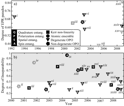
Figure 9: a) A history of experiments investigating measure of: a) $\mathcal{E}^{2}$, the EPR paradox (Eq. (23)) and b) inseparability $D$ (Eqs. (34) and (21)), for continuous variable measurements. Where $D<0.5$, one can infer an EPR paradox, using $\mathcal{E}\leq 2D$ (Section VI). The grey labels in (a) indicate that $\mathcal{E}^{2}$ has not been measured directly, but is inferred by the authors. From (b) we see that an EPR paradox could have been inferred in other experiments as well. ($i$) Ou et al. (1992), ($ii$) Zhang et al. (2000))[Inferred from a variance product measurement], ($iii$) Silberhorn et al. (2001), ($iv$) Julsgaard et al. (2001), ($v$) Schori et al. (2002), ($vi$) Bowen et al. (2002b), ($vii$) Bowen et al. (2003a), ($viii$) Glöckl et al. (2003), ($ix$) Josse et al. (2004), ($x$) Hayasaka et al. (2004), ($xi$) Takei et al. (2005), ($xii$) Laurat et al. (2005), ($xiii$) Wenger et al. (2005), ($xiv$) Huntington et al. (2005), ($xv$) Villar et al. (2005), ($xvi$) Nandan et al. (2006), ($xvii$) Jing et al. (2006), (xviii) Takei et al. (2006), (xix) ichiro Yoshino et al. (2007), (xx) Zhang et al. (2007), (xxi) Dong et al. (2007), (xxii) Keller et al. (2008), (xxiii) Grosse et al. (2008), (xxiv) Wagner et al. (2008), (xxv) Boyer et al. (2008). Inseparability has also been verified using other measures, such as negativity (Ourjoumtsev et al. (2007)).

The Einstein-Podolsky-Rosen gedanken-experiment has been realized through a series of important developments, both theoretical and technological. Experiments have measured violation of the inferred Heisenberg uncertainty principle, thus confirming EPR-entanglement. Fig. 9 summarizes the degree of entanglement and the degree of EPR paradox achieved in continuous variable experiments to date.

A question often arising is the utility of such measurements, given that Bell inequality violations are a more powerful indication of the failure of local realism. There are multiple reasons for this. The beauty of the EPR approach is its simplicity, both from a theoretical and a practical point of view. Bell inequalities have proved in reality exceedingly difficult to violate. EPR measurements with quadratures do not involve conditional state preparation or the inefficient detectors found in most current photon-based Bell inequality experiments, and the issue of causal separation does not look insurmountable.

The development of these techniques also represents a new technology, with potential applications in a number of areas ranging from quantum cryptography and ultra-precise measurements, through to innovative new experimental demonstrations of ideas like quantum ‘teleportation’ - using entanglement and a classical channel for transmission of quantum states between two locations.

Owing to Bell’s theorem, Einstein et al.’s argument for completing quantum mechanics is sometimes viewed as a mistake. Yet there exist alternatives to standard quantum theory which are not ruled out by any Bell experiments. These include spontaneous decoherence (Ghirardi et al. (1986); Bassi and Ghirardi (2003)), gravitational nonlinearity (Penrose (1998); Diósi (2007)), and absorber theories (Pegg (1997)). By using field-quadrature measurements and multi-particle states, quantum theory and its alternatives can be tested for increasingly macroscopic systems (Marshall et al. (2003)). However, an ingredient central to the EPR argument, causal separation of measurement events, is missing from these experiments to date. In view of this, further EPR experiments are of considerable interest, especially with causal separation and/or massive particles.