OBSERVATIONS OF DOPPLER SHIFT OSCILLATIONS WITH THE EUV IMAGING SPECTROMETER ON HINODE

Abstract

Damped Doppler shift oscillations have been observed in emission lines from ions formed at flare temperatures with the Solar Ultraviolet Measurements of Emitted Radiation spectrometer on the Solar and Heliospheric Observatory and with the Bragg Crystal Spectrometer on Yohkoh. This Letter reports the detection of low-amplitude damped oscillations in coronal emission lines formed at much lower temperatures observed with the EUV Imaging Spectrometer on the Hinode satellite. The oscillations have an amplitude of about 2 km s^-1, and a period of around 35 min. The decay times show some evidence for a temperature dependence with the lowest temperature of formation emission line (Fe XII 195.12 Å) exhibiting a decay time of about 43 min, while the highest temperature of formation emission line (Fe XV 284.16 Å) shows no evidence for decay over more than two periods of the oscillation. The data appear to be consistent with slow magnetoacoustic standing waves, but may be inconsistent with conductive damping.

1. INTRODUCTION

In recent years, oscillatory phenomena have been detected in the solar corona using spacecraft imaging instruments (e.g., Aschwanden et al., 1999; Schrijver et al., 2002) and spectroscopic instruments (e.g., Wang et al., 2002; Kliem et al., 2002; Mariska, 2006). Detection and characterization of coronal oscillatory phenomena with spectroscopic instruments that simultaneously capture many emission lines is particularly important, since it offers the possibility of refining our understanding of the temperature-dependent behavior of the oscillations. It may also be possible to make simultaneous observations in density-sensitive pairs of emission lines, further constraining the characteristics of the oscillations.

The EUV Imaging Spectrometer (EIS) on Hinode produces stigmatic spectra in two 40 Å wavelength bands centered at 195 and 270 Å. EIS can image the Sun using 1″ and 2″ slits to produce line profiles and 40″ and 266″ slots to produce monochromatic images. When the slits are used, the EIS mirror can be moved to construct spectroheliograms by rastering an area of interest. This can provide a snapshot of the thermal structure and dynamics of a region of interest, but with typical exposure times ranging from a few seconds to a minute or more, it is difficult to obtain high time cadence dynamical data in this manner. When a higher cadence is important, EIS can operate in a sit-and-stare mode in which the slit covers a fixed location on the Sun and takes repeated exposures. A more global context can then be provided by preceding and/or following the sit-and-stare data with EIS spectroheliograms. Further context is often available from observations taken simultaneously with the Hinode X-Ray Telescope (XRT). An overall description of EIS is available in Culhane et al. (2007), XRT is described in Golub et al. (2007), and the Hinode mission is described by Kosugi et al. (2007).

In this Letter we show that damped oscillations are present in some spectral lines observed in sit-and-stare observations taken with EIS. While the earlier spectroscopic observations detected oscillations in plasma at flare temperatures (e.g., Wang et al., 2003; Mariska, 2006), the data presented here show the presence of oscillations at typical active region temperatures. The oscillations appear to be standing slow mode magnetoacoustic waves, but the temperature dependence of the decay times may be inconsistent with conductive damping.

2. EIS OBSERVATIONS

The observations discussed in this paper were centered at the southwest limb (S09W84) on 2007 January 14. A sit-and-stare observation began at 12:30:12 UT and consisted of 120 exposures with the 1″ slit, each with an exposure time of 60 s. Each exposure covered nine data windows on the EIS detectors. This Letter only presents the results from lines in six of those windows. Data from the other detector windows were not suitable for a Doppler shift analysis, either because of weak signal or difficult to fit line profiles. Each window was 32 spectral pixels wide and covered a height of 512″ in the N/S direction. EIS detector pixels are 22.3 mÅ wide in the spectral direction and 1″ wide in the spatial direction. The measured FWHM for the instrument at 185 Å is 47 mÅ (Culhane et al., 2007).

The EIS sit-and-stare observation was followed by a spectroheliogram taken with the 1″ slit and covering a $240\arcsec\times 240\arcsec$ region. This data set contained 12 spectral windows, including all of those covered in the sit-and-stare observation. The exposure times, however, were only 5 s, resulting in a relatively weak signal in some of the lines over much of the spectroheliogram.

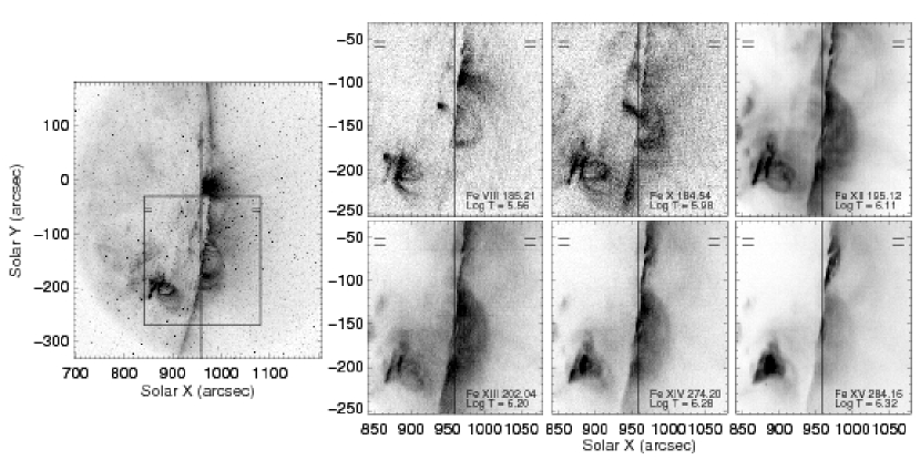
Figure 1.— A TRACE 171 Å image taken at 11:19:41 UT showing the location of the EIS sit-and-stare observation taken from 12:30:12 to 14:32:58 UT on 2007 January 14 and the EIS spectroheliograms obtained from 14:50:12 to 15:16:22 UT, which are shown to the right of the TRACE image. Short horizontal lines on the raster outline and on each image mark the $y$-range of the rows in the EIS spectroheliogram that show Doppler-shift oscillations.

While the XRT was making exposures during the time of the EIS sit-and-stare observation, the exposure times were very short, resulting in images with significant detail only for the strongest features. The Transition Region and Coronal Explorer (TRACE) was also observing at this location and provided better context images. The left side of Figure 1 shows a TRACE 171 Å image of the area around the sit-and-stare data set with the locations of the EIS slit for the sit-and-stare observation and the following EIS raster indicated. Also marked is the $y$-range of the locations in the EIS raster that exhibit the oscillations discussed in this Letter.

All the EIS data were processed to remove detector bias and dark current, hot pixels and cosmic rays, and calibrated using the the prelaunch absolute calibration, resulting in intensities in ergs cm^-2 s^-1 sr^-1 Å^-1. The EIS slit tilt and orbital variation in the line centroids were also removed from the data. The emission lines in each spectral window were then fitted with Gaussian profiles, providing the total intensity, location of the line center, and the width. The data in the long wavelength detector were also shifted by 17 pixels in the $y$-direction to correct for the offset between the two detectors.

The right panels in Figure 1 show the appearance of the area covered by the EIS spectroheliogram in the lines contained in the sit-and-star observation along with the location of the EIS slit for the sit-and-stare observation. Beneath the identification of each emission line, we also list the log of the temperature of formation of the line.

Since the spacecraft was in a fixed pointing mode during both the sit-and-stare observation and the following spectroheliogram, the sit-and-stare slit location on the spectroheliogram is well determined. Placing the slit on the TRACE image is more challenging. That placement has been accomplished using the feature centered at an $(x,y)$ location of about $(880,-200)$. The placement is only accurate to a few arcseconds.

As we mentioned above, because short exposure times were used, the XRT images only showed the brightest features. Examination of a movie of the images, however, does show flare-like brightenings taking place in the small loop-like features at ($x$, $y$) locations of roughly ($850$, $-150$) and ($860$, $-130$) visible in the Fe XII image and those formed at higher temperatures. One of these events, which took place at roughly 13:00 UT, resulted in a brightening in the the feature used to co-align with the TRACE image and appeared to show a very weakly emitting loop that connected to the area that exhibited oscillations. Thus, we believe that the observed oscillations are the result of impulsive heating events and that the sit-and-stare data are near one footpoint of the impulsively heated loops. Note that the event at 13:00 UT can not be the one that generated the observed oscillations, since they are already present in the EIS data by that time.

3. RESULTS

Figure 2 shows a color representation of the measured centroid positions for each spectral line as a function of time. For many $y$-positions, the Doppler shift appears to be relatively constant as a function of time. There are, however, a number of positions that exhibit time-dependent behavior. Perhaps the most striking is the marked region near a $y$-position of $-60\arcsec$, which in the three higher temperature lines shows a pattern of alternating redshifted and blueshifted emission in the Doppler-shift data and some evidence for a gradual change in the intensity data. A second position range showing similar behavior is indicated near the bottom of the figure.

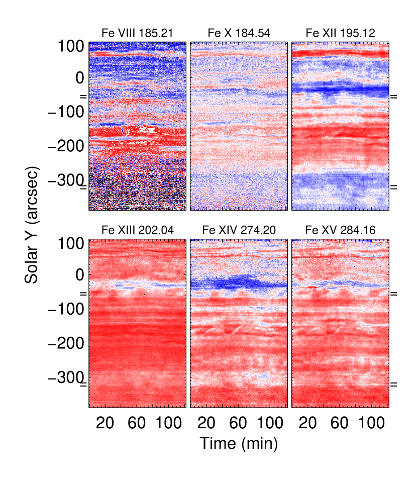
Figure 2.— EIS sit-and-stare Doppler-shift data in six different emission lines obtained beginning at 12:30:12 UT on 2007 January 14. The horizontal axis shows the start times of the exposures relative to the beginning of the data set. The Doppler shift in each window is adjusted so that the zero value is the average over the window. The maximum and minimum values plotted in each case are $+20$ and $-20$ km s^-1, respectively. The short horizontal lines mark the ranges of rows showing Doppler-shift oscillations.

To examine further the signal in this portion of the Doppler-shift data, we have averaged the measured total line intensities and centroid shifts in each detector window over the seven rows centered on a $y$-position of $-56\arcsec$.

The four higher temperature lines show clear evidence in the Doppler shift averages for and oscillatory pattern, which we fit with a combination of a polynomial background and a damped sine wave of the form

$$v(t)=A_{0}\sin(\omega t+\phi)\exp(-\lambda t)+B(t),$$ (1)

where

$$B(t)=b_{0}+b_{1}t+b_{2}t^{2}+b_{3}t^{3}+\dots$$ (2)

The top and bottom panels of Figure 3 show the behavior of the averaged intensities and the detrended averaged Doppler shifts in these lines, respectively. Also shown on each of the bottom panels is the best-fit damped sine wave. Only the data in the interval between the vertical dashed lines was used for the fitting. Both a linear and a quadratic background yielded similar fitting parameters for the damped sine wave, with the quadratic fit being slightly better in some cases. The reduced $\chi^{2}$ for the fits are generally around 2.

The averaged line intensities for the two cooler lines, especially the Fe XII 195.12 Å emission line, show some evidence for periodic intensity fluctuations, particularly over the first portion of the interval used for fitting the Doppler shift data. We have, however, been unable to fit a decaying sine wave to the data using equation (1).

Figure 3.— Averaged intensity and detrended Doppler-shift data for the emission lines that exhibited Doppler-shift oscillations. The curves on the lower plots show the best-fit to a decaying sine wave.

Examination of the averaged Doppler shift data in the Fe VIII 185.21 Å emission line shows no evidence for oscillatory behavior. The data for the Fe X 184.54 Å emission line shows an indication of a small disturbance in the line centroid at the time the oscillations are observed in the higher temperature lines. Thus the oscillation does not appear to be present for lines with temperatures of formation of less than about 1 MK.

Table 1 summarizes the parameters of the fits to the Doppler shift data. For all the lines in the Table, the amplitudes, periods, and phases are roughly similar, suggesting that we are seeing the response of the solar plasma to the same disturbance. Note, however, that there appears to be a tendency for the decay time to increase with increasing temperature of formation for the line. The data for the Fe XV 284.16 Å line are consistent with no detectable decay over the time interval measured.

Table 1Fitting Results

	$A_{0}$	$\omega$	$\phi$	$\lambda$
Line	(km s-1)	(rad min-1)	(rad)	(hr-1)
Fe xii	$2.1\pm 0.2$	$0.181\pm 0.003$	$-0.1\pm 0.1$	$1.4\pm 0.2$
Fe xiii	$3.7\pm 0.4$	$0.168\pm 0.003$	$+0.2\pm 0.1$	$1.2\pm 0.2$
Fe xiv	$2.5\pm 0.3$	$0.171\pm 0.002$	$-0.1\pm 0.1$	$0.62\pm 0.15$
Fe xv	$1.8\pm 0.2$	$0.179\pm 0.002$	$-0.7\pm 0.1$	$-0.05\pm 0.13$

4. DISCUSSION AND CONCLUSIONS

Defining the maximum amplitude displacement for the oscillations (Wang et al., 2003) as

$$A=A_{0}/(\omega^{2}+\lambda^{2})^{1/2},$$ (3)

we calculate a value for $A$ in the Fe XIV 274.20 Å line of about 860 km. Thus, if the oscillations are transverse to the line of sight, the range of motion would only be on the order of 1″, making them very difficult to detect in images.

The Doppler shift data shown in Figure 3 looks similar to the Doppler shift oscillations observed with the Solar Ultraviolet Measurements of Emitted Radiation instrument (SUMER) on the Solar and Heliospheric Observatory (SOHO) (e.g., Wang et al., 2003). Those oscillations were primarily seen in emission lines from Fe XIX and Fe XXI and appeared to be the response to flare-like heating in active region loops. The amplitudes were much larger than those reported here—averaging about 98 km s^-1. The average period reported was 17.6 min, but ranged up to 31.1 min.

As we discussed in §2, we believe that the observed oscillation is the result of a heating event in a nearby structure that appears to be magnetically connected to the area where the oscillations are observed. Assuming we are observing a loop, that the oscillations are near one footpoint and that the other footpoint is at an ($x$, $y$) position of approximately ($860$, $-130$), we compute a distance between the two footpoints of roughly 218 Mm. A semicircular loop with this diameter would then have a length of approximately 342 Mm. For a sound speed of 200 km s^-1, the sound travel time between the footpoints is about 29 min. This is within a factor of two of the value expected for a standing magnetoacoustic wave oscillating in the fundamental mode. Since the locations of the footpoints are highly uncertain, especially since they are very close to the limb, and the loop geometry is difficult to determine, we believe this this level of agreement is good and suggests that we are observing a damped standing mode slow magnetoacoustic wave.

A strong indicator that the oscillations are standing mode would be the presence of a $1/4$ period phase shift between the intensity and the Doppler shift (Sakurai et al., 2002). Both the Fe XII and Fe XIII line intensities show local peaks at about 10 and 20 min into the interval used for fitting the Doppler shift data, suggesting a period for any intensity oscillation of about 10 min. The Fe XIV and Fe XV emission lines show local peaks at about 30 and 50 min into the fitting interval, suggesting a period for any intensity oscillation of of about 20 min. In both cases, these periods are shorter than those listed in Table 1. For a sound wave, $v=c_{s}\delta\rho/\rho$, where $c_{s}$ is the sound speed and $\rho$ is the density. Thus, for the formation temperatures of the lines showing Doppler shift oscillations, $\delta\rho/\rho\approx 0.01$, a very small density fluctuation, which would not be detectable at the signal-to-noise levels in the intensity data. Thus, we believe that the most that can be said about the observed intensities is that they are not inconsistent with standing mode slow magnetoacoustic waves.

The ratio of the decay time to the wave period can provide some additional information on the damping mechanism. For the SUMER oscillations the average value for that ratio is 0.85 (Wang et al., 2003). For the three cooler lines in Table 1 the values are 1.2, 1.3, and 2.6, respectively, with the value for the Fe XV line being greater than 2.8. The result that the ratio for the Fe XV line is potentially much larger than that for the other three lines would be inconsistent with the conclusion from SUMER observations that the observed slow magnetoacoustic waves are damped by thermal conduction (Ofman & Wang, 2002). Because of the strong temperature dependence of the thermal conductivity, we would expect the damping rate to increase with increasing temperature (Porter et al., 1994).

Because the corona is threaded with a magnetic field, a diverse array of oscillation modes is possible (e.g., Roberts, 2000; Roberts & Nakariakov, 2003). The sensitivity and temperature coverage of EIS, especially when combined with the high time cadence imaging that XRT can provide, opens up the possibility of detecting new wave modes and new excitation mechanisms. Similarly, this increased sensitivity may make it possible to detect additional dissipation mechanisms. For example, recent work by Ofman (2007) and Selwa et al. (2007) show that wave leakage may be important in the complex magnetic geometries of active regions.

While EIS is capable of detecting Doppler shifts of of less than 0.5 km s^-1, the result is dependent on an accurate removal of the orbital Doppler shift fluctuation, which has an amplitude of about 20 km s^-1. Since the observation took place over more than one orbit of the spacecraft, the orbital variation can be accurately modelled and we believe it has been correctly removed. In addition, the Hinode pointing exhibits a jitter in both the $x$ and $y$ directions that can have a range of up to 4″ over a 120 min observation. We have looked at the jitter over the period of the sit-and-stare observation and see no evidence for any correlation between the jitter and the detected oscillations. Note, however, that this jitter means that the EIS 1″ slit is averaging over more than 1″ in both $x$ and $y$ during the observation. The fact that we see the oscillation taking place over at least seven pixels in the $y$-direction suggests that the oscillating structures are sizable, and the jitter should not cause a significant problem.

To further verify this observation, we have performed the same analysis on the oscillatory Doppler-shift signal marked in the lower portions of Figure 2. The oscillations observed over that position range (nine pixels), have similar amplitudes, a shorter period (about 25 min), and similar damping times. There is, however, less evidence for a temperatures dependence to the ratio of the damping time to the period. We believe that this second event in this EIS sit-and-stare data set confirms the presence of these oscillations at active region temperatures, but shows the need for additional studies on the damping mechanism.

References

- Aschwanden et al. (1999) Aschwanden, M. J., Fletcher, L., Schrijver, C. J., & Alexander, D. 1999, ApJ, 520, 880
- Culhane et al. (2007) Culhane, J. L., et al. 2007, Sol. Phys., 243, 19
- Golub et al. (2007) Golub, L., et al. 2007, Sol. Phys., 243, 63
- Kliem et al. (2002) Kliem, B., Dammasch, I. E., Curdt, W., & Wilhelm, K. 2002, ApJ, 568, L61
- Kosugi et al. (2007) Kosugi, T., et al. 2007, Sol. Phys., 243, 3
- Mariska (2006) Mariska, J. T. 2006, ApJ, 639, 484
- Ofman (2007) Ofman, L. 2007, ApJ, 655, 1134
- Ofman & Wang (2002) Ofman, L., & Wang, T. 2002, ApJ, 580, L85
- Porter et al. (1994) Porter, L. J., Klimchuk, J. A., & Sturrock, P. A. 1994, ApJ, 435, 482
- Roberts (2000) Roberts, B. 2000, Sol. Phys., 193, 139
- Roberts & Nakariakov (2003) Roberts, B., & Nakariakov, V. M. 2003, in NATO Science Series: II: Mathematics, Physics and Chemistry, Vol. 124, Turbulence, Waves and Instabilities in the Solar Plasma, ed. R. Erdelyi, K. Petrovay, B. Roberts, & M. J. Aschwanden (Kluwer Academic Publishers, Dordrecht), 167–192
- Sakurai et al. (2002) Sakurai, T., Ichimoto, K., Raju, K. P., & Singh, J. 2002, Sol. Phys., 209, 265
- Schrijver et al. (2002) Schrijver, C. J., Aschwanden, M. J., & Title, A. M. 2002, Sol. Phys., 206, 69
- Selwa et al. (2007) Selwa, M., Ofman, L., & Murawski, K. 2007, ApJ, 668, L83
- Wang et al. (2002) Wang, T., Solanki, S. K., Curdt, W., Innes, D. E., & Dammasch, I. E. 2002, ApJ, 574, L101
- Wang et al. (2003) Wang, T. J., Solanki, S. K., Curdt, W., Innes, D. E., Dammasch, I. E., & Kliem, B. 2003, A&A, 406, 1105