Introduction

About ten years ago the primary communications regarding two significant astrophysics discoveries were appeared. Two independent research groups announced in 1998–1999 [1, 2] about the detection of the peculiar deviations from the Hubble law linearity near the cosmological red shift value equal to $z_{exp}=0.46\pm 0.13$. At 1998 the information was published [3] (see also [4]) about the reliable experimental registration of the systematic uniform anomalous blue frequency drift in the radiosignals received from the spacecrafts Pioner 10/11 leaving the Solar system (Pioneer Anomaly — PA).

The standard treation of the first of these phenomena leads to a predominance (more than 65 % from the total energy amount) of the paradoxical dark energy in contemporary Methagalaxy. The conventional treation of the observable PA-effect as a common Doppler shift is nessesarily presumed the existence of some additional uniform sunward acceleration having the magintude equal to $a_{p}=(8.74\pm 1.33)\cdot 10^{-8}\ \frac{\mbox{\small cm}}{\mbox{\small s}}$ experienced by the spacecrafts. In spite of the abundant theoretical suppositions concerning the possible source of such an acceleration the origin of the Pioneer Anomaly remains unexplained up to now [5].

The proximity of $a_{p}$ to the quantity $W_{0}=cH_{0}$ ($c$ is the speed of light, $H_{0}$ is the Hubble constant) was noted by several authors. However, any unambiguous theoretical arguments in favor of the possible existence of such a connection are absent up to now.

In the present report the description of the cosmological expansion and its possible local manifestations is given via treating the proper conformal transformations as a coordinate transformation from a comoving Lorentz RF to an uniformly accelerated RF. Such an approach permit to derive the explicit analytic expression for the Hubble law, which allows to connect the acceleration with the Hubble constant as well as to reproduce the Accelerating Universe and Pioneer Anomaly effects in exact correspondence with the observations. These effects, once dictated by the conformal time inhomogeneity, can be interpreted as the manifestations of the background acceleration existence, i.e., of the noninertial character of any physical frame of reference which is coupled locally to an arbitrary point of the modern Metagalaxy.

The topics of the present report are as follows.

• Conformal transformations and the accelerating frame of reference.

• Conformal deformation of the light cone and time inhomogeneity.

• The dependence of distance on the red shift.

• The Hubble law. Connection between the Hubble constant and the background acceleration.

• Accelerating Universe effect without Dark Energy.

• The universal blue-shifted frequency drift. Pioneer Anomaly.

I. Conformal transformations and the accelerating frame of reference

It is well known that the special conformal transformations (SCT)

$$x^{\prime\mu}=\frac{x^{\mu}+a^{\mu}(x^{\alpha}x_{\alpha})}{1+2(a^{\alpha}x_{\alpha})+(a^{\alpha}a_{\alpha})(x^{\beta}x_{\beta})},$$

where $a^{\mu}$ is the four-vector parameter, $\eta_{\mu\nu}=\mathrm{diag}(1,-1,-1,-1)$, can be interpreted as the transformations between the Lorentz (comoving) frame of reference $S(x^{\mu})$ and the noninertial (accelerated) frame of reference $S^{\prime}(x^{\prime\mu})$ (see, for example, [6]). Following [6] we shall for simplicity consider a two-dimensional subspace $\{t,x\}$, i.e. we put

$$x^{\mu}=(ct,x,0,0),\ a^{\mu}=(0,-\frac{w}{2c^{2}},0,0),$$

where $w$ is a constant uniform acceleration. In general $a^{\mu}$ is related with a constant 4-acceleration $w^{\mu}$ as follows $a^{\mu}=w^{\mu}/2c^{2}$.

It is conveniently to write the transformations (1) in the following noncovariant form:

$$\left.\begin{gathered}x^{\prime}=\frac{x\xi-\frac{wt^{2}}{2}}{\xi^{2}-\eta^{2}},\\ t^{\prime}=\frac{t}{\xi^{2}-\eta^{2}},\end{gathered}\right\}$$

where

$$\xi=1+\frac{wx}{2c^{2}},\qquad\eta=\frac{wt}{2c},\qquad r_{0}=c^{2}/w.$$

In the case when $\frac{wx}{2c^{2}}$ and $\frac{wt}{2c}$ are negligible we have from (3)

$$x^{\prime}=x-\frac{wt^{2}}{2},\qquad t^{\prime}=t,$$

which corresponds to Galilei-Newton kinematics. It is also clear from (3) that sign $(-)$ of the vector’s $a^{\mu}$ $x$-component describes a positive direction of $S^{\prime}$ acceleration along the $x$-axis of the inertial reference frame (IRF) $S$.

The velocity and acceleration transformations laws are presented in [7]. In the approximation $\xi\approx 1,\ \eta\ll 1$ this transformation leads to formulae

$$V^{\prime}_{x}=V_{x}-wt,$$

for the velocities and to

$$w^{\prime}_{x}=w_{x}-w$$

for the accelerations in the correspondence with Galilei-Newton kinematics.

From (5), the existence of blue Doppler drift follows immediately. Really, due to (5) the longitudinal component of a point velocity $V^{\prime}_{x}$ measured by an observer fixed in non-inertial RF $S^{\prime}$ will be less then that measured by an observer fixed in the inertial comoving RF $S$ by $\Delta V_{x}=wt$.

Therefore, for the observed blue shift we have

$$\Delta\nu_{obs}=\nu^{\prime}-\nu_{mod}=\nu_{0}\frac{wt}{c},$$

where $\nu_{0}$ is the signal frequency emitted by a source fixed in $S$ and $\nu_{mod}$ is the frequency defined by neglecting non-inertiality of $S^{\prime}$. In the approximation considered the shift is linear in time. The rate of shift $\dot{\nu}_{obs}=\frac{d\nu_{obs}}{dt}$ is defined by the following simple relation

$$\dot{\nu}_{obs}=\nu_{0}\frac{w}{c}.$$

This result, in principle, is well known. Here we have to do, in fact, with the effect of the gravitational (Einstein) frequency drift described on the basis of the equivalence principle.

The relation (6) holds in every comoving RF as long as in this frame $\xi\approx 1,\ \eta\ll 1$ approximation is valid. A probe particle free of dynamical influence in the comoving RF, i.e. with $W_{x}=0$, in accordance with (5) will be uniformly accelerated in the non-inertial RF $S^{\prime}$ with the constant acceleration of $-w$. Such an acceleration can be registered by any observer fixed in any point of this non-inertial RF $S^{\prime}$. By the equivalence principle the non-inertial observer is entitled to identify this acceleration with an existence of a constant (background) gravitational field which results in acceleration $w$.

This result can be confirmed via dynamical approach using the expression of the conformal one-particle Lagrangian as it shown in [8]. Following a common practice for the Lagrangian dynamical description in the noninertial RF the following expression for the one-particle nonrelativistic Lagrangian can be obtained

$$L_{NR}=\frac{m_{0}\vec{v}^{2}}{2}-\frac{m_{0}c^{2}}{R_{u}}r.$$

where

$$R_{u}=r_{0}=\frac{c^{2}}{w}.$$

The term $\frac{m_{0}c^{2}}{R_{u}}r$ in (9) can be treated in the correspondence with the equivalence principle as a potential energy of the probe mass $m_{0}$ in the following ”gravitational” potential:

$$\varphi_{0}=\frac{c^{2}}{R_{u}}r=wr.$$

This potential plays the role of the source of the background uniform acceleration having the magnitude $w=w_{background}$ and directed towards the point of observation.

II. Conformal deformation of the light cone and time inhomogeneity

Now we consider the transformations of the light cone generatrices under SCT (1). Since $x^{\prime\mu}x^{\prime}_{\mu}=x^{\mu}x_{\mu}(1+2(ax)+(a)^{2}(x)^{2})^{-1}$, transformations (1) leave the light cone equation invariant, i.e., from $x^{\mu}x_{\mu}=0$ follows $x^{\prime\mu}x^{\prime}_{\mu}=0$. However the light cone surface is deformed non-linearly. From (1), it generally follows

$$x^{\prime\mu}=\frac{x^{\mu}}{1+2(ax)},$$

when additionally $x^{\mu}x_{\mu}=x^{\prime\mu}x^{\prime}_{\mu}=0$.

In the two-dimensional case considered we have the relation

$$t^{\prime}_{\pm}=\frac{t}{1\pm\frac{t}{t_{lim}}},$$

where $t_{lim}=c/w$.

The choice of sign corresponds to signal propagation in the forward and backward directions, respectively. We are reminded that the symbol $t$ ($t^{\prime}$) represents time of a light signal propagation between two spatially separated points in the space of Lorentz RF $S$ (in the non-inertial RF $S^{\prime}$). So the quantities $R=ct$ and $R^{\prime}=ct^{\prime}$ define location distances in both of these RFs.

Obviously a semi-infinite time interval $0\leqslant t<\infty$ corresponding to the positive (forward) direction of signal propagation maps onto a finite time interval $0\leqslant t^{\prime}_{+}\leqslant t_{lim}$. For the backward direction, on the contrary, a finite interval $0\leqslant t\leqslant t_{lim}$ maps onto a semi-infinite time interval $0\leqslant t^{\prime}_{-}<\infty$ (Fig. 1).

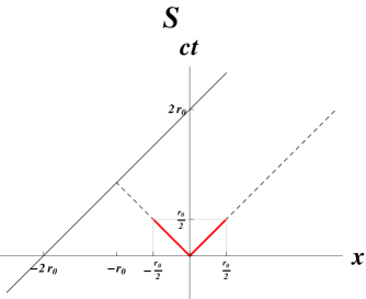
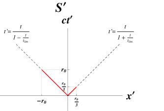
Fig. 1: Conformal deformation of the light cone. Initially equal intervals $t_{\pm}=\frac{t_{lim}}{2}$ of forward and backward generatrices transform into unequal intervals $t^{\prime}_{+}=\frac{t_{lim}}{3}$ and $t^{\prime}_{-}=t_{lim}$.

The non-linear time transformation (12) will further be referred to as the conformal deformation of time, or conformal time inhomogeneity.

III. The dependence of distance on the red shift

First and foremost we show that transformations (12) allow us to obtain an explicit expression for location distance as a simple function of red shift $z$.

Let us consider, on the basis of the formula (12), the case of a signal propagation from the deep past to the point of the observer position. That means that we choose the lower sign in the formula (12):

$$t^{\prime}=\frac{t}{1-\frac{t}{t_{lim}}},$$

where $t_{lim}=c/w$, and $t$ is the time of the signal propagation to the point of observation.

First of all, from (13) we obtain the explicit expression for the time interval of the signal propagation as a function of the red shift $z$.

From (13), we have, for small time increments $\Delta t^{\prime}$ and $\Delta t$, the following expression

$$\Delta t^{\prime}=\Delta t(1-\frac{t}{t_{lim}})^{-2}.$$

If $\Delta t$ and $\Delta t^{\prime}$ are the periods of oscillations of the emitted ($\Delta t=T_{emitted}$) and received ($\Delta t^{\prime}=T_{observable}$) signals, respectively, then, using the standard definition of the red shift

$$\frac{\lambda_{observable}}{\lambda_{emitted}}=z+1,$$

where $\lambda_{observable}=cT_{observable}$ and $\lambda_{emitted}=cT_{emitted}$, we find, from (14), the expression

$$\frac{\lambda_{observable}}{\lambda_{emitted}}=(1-\frac{t}{t_{lim}})^{-2}=z+1,$$

which gives

$$t(z)=t_{lim}\frac{(z+1)^{1/2}-1}{(z+1)^{1/2}}.$$

Here $t(z)$ represents the time interval between the moments of emitting and receiving the light (electromagnetic) signal. So, assuming that the speed of light is constant and does not depend on the velocity of the emitter, the quantity $R=ct$ can be regarded as the distance covered by the signal.

From the formula (17), we obtain an expression which determines the explicit form of dependence of $R$ on the red shift $z$:

$$R(z)=R_{u}\frac{(z+1)^{1/2}-1}{(z+1)^{1/2}}=R_{u}\left(1-\frac{1}{(z+1)^{1/2}}\right).$$

Here$R_{u}=ct_{lim}$ is a parameter, which, within the model suggested, has the sense of the limit (maximal) distance.

The quantity $R(z)$ defined by (18) corresponds to the distance, which in cosmology is referred to as a location distance. In principle, the relation (18) allows for a direct experimental verification in the whole range of $z$ variation, and can be confirmed or refused by observations. We are to emphasize the essentially kinematic nature of the relation (18). It is the manifestation of the nonlinear conformal time deformation (12) which follows from Special Conformal Transformations exactly in the same manner as the Doppler effect, and the dependence $V(z)$ follows from the linear time deformation arising from the Lorentz boosts leaving the equation of light cone unaltered. The question of the connection between R(z) and the spectrometric (photometric) distance adopted in the standard astrophysics calls for special investigation.

IV. The Hubble law. Connection between the Hubble constant and the background acceleration

Now, we can obtain the explicit expression for the Hubble law. Using (18) and the known expression for the function $V(z)$:

$$\frac{V(z)}{c}=\frac{(z+1)^{2}-1}{(z+1)^{2}+1}.$$

We can find the following expression for the ratio $V/R$:

$$\frac{V(z)}{R(z)}=cR_{u}^{-1}f(z),$$

where

$$f(z)=\frac{(z+1)^{1/2}}{(z+1)^{2}+1}\cdot\frac{(z+1)^{2}-1}{(z+1)^{1/2}-1}.$$

It is easy to see that $\lim_{z\rightarrow 0}f(z)=2$.

In this limit we obtain the conventional expression for the Hubble law:

$$V=H_{0}R,$$

where $H_{0}$ is the Hubble constant.

By comparing this formula with $\lim_{z\rightarrow 0}\frac{V(z)}{R(z)}$ from formula (20), we can establish the following connection between the acceleration $w$ and the Hubble constant $H_{0}$:

$$2cR_{u}^{-1}=2w/c=H_{0}.$$

It is seen that the relation (12) defining the conformal time inhomogeneity allows us to establish the following simple connection between the parameter $w$ defining the background acceleration and the Hubble constant $H_{0}$

$$w=\frac{1}{2}cH_{0}.$$

Hence, in the considered approach the constant acceleration $w$ intrinsic to non-inertial RF $S^{\prime}$ can naturally be connected to the Hubble constant $H_{0}$, defining space expansion.

V. Accelerating Universe effect without Dark Energy

Now we analyze the general relation (20) for $V(z)/R(z)$. Taking into account the connection (22) between $R_{u}$ and the Hubble constant $H_{0}$, we rewrite this equation in the dimensionless form as

$$\phi(z)=\frac{V(z)}{H_{0}R(z)}=\frac{1}{2}\frac{(z+1)^{1/2}}{(z+1)^{2}+1}\cdot\frac{(z+1)^{2}-1}{(z+1)^{1/2}-1}.$$

The function $\phi(z)$ is shown in Fig. 2. Horizontal line in represents strict Hubble law (21). This function possesses a maximum at $z_{0}\cong 0.475$. Overall variation of $\phi(z)$ demonstrates that in the interval $0\leq z<z_{0}$ the distance $R(z)$ increases with $z$ more slowly, and in the interval $z_{0}<z<\infty$ approaches its limit value $R_{u}$ more rapidly, than the velocity $V(z)$ approaches its limit $c$ (Fig. 3). We see that from the point of view of the proposed approach the origin of this maximum has the pure kinematic origin.

Fig. 2: The function $\phi(z)$.

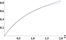
Fig. 3: Functions $V(z)/c$ (dashed line) and $R(z)/R_{u}$ (solid line). The values of the both functions coincide at the points of $z=0$ and $z\approx 1.315$. The inequality $V(z)/c>R(z)/R_{u}$ ($V(z)/c<R(z)/R_{u}$) takes place in the interior (exterior) of this interval.

As regards a possible treatment of the behavior of the function $\phi(z)$ in terms of the standard dynamical GR approach using the decelaration parameter, we are to notice the following. According to the pure kinematic approach proposed in our paper, the source of the effects induced by the cosmologic expansion is the conformal time inhomogeneity. The “acceleration” attributed to the emitting source arises because of treating the actual nonlinear time dependence $t^{\prime}(t)$ in terms of the traditional theoretical paradigm based on the time homogeneity concept.

The interpretation of $\phi(z)$ behavior from the point of view of common treatment seems as follows. In the interval $\infty>z>z_{0}$, there is deceleration $\left(\frac{d\phi}{dz}<0\right)$ of cosmological expansion, which turns to acceleration $\left(\frac{d\phi}{dz}<0\right)$ at $z_{0}\cong 0{,}475$. Numerical value of $z_{0}$ agrees quite well with experimentally founded ”point of change” $z_{exp}=0.46\pm 0.13$.

It should be emphasized that the basic formula (12) for the conformal transformations of the time, as well as all its consequences, are valid on the assumption that the Hubble parameter $H_{0}$ is constant. Hopefully this assumption is reasonable as applied to at least later stages of the Universe evolution. In this case the proposed formulae (18) and (20) can be valid for the experimentally obtained values of the read shift having the order of several units.

It would be of interest to compare the obtained expression (24) for the function $V(z)/R(z)$ with such one which can be derived at once from the basic correlation

$$\frac{R_{today}}{R_{emitted}}=\frac{\lambda_{today}}{\lambda_{emitted}}=z+1$$

adopted in the contemporary cosmology. Here $R_{today}$ and $R_{emitted}$ are the Universe linear sizes at the instant of the reception and the emission of the electromagnetic signal correspondingly.

Defining the location distance in the euclidean approximation i. e. neglecting the spatial curvature and using the definition (25) we obtain the condition $R_{L}(z)=R_{today}\frac{z}{z+1}$, and taking into account the formula (19) defining $V(z)$ we come to the following expression:

$$\frac{V(z)}{R_{L}(z)}=cR_{today}\varphi(z),$$

where

$$\varphi(z)=\frac{(z+1)^{2}-1}{z}\cdot\frac{(z+1)}{(z+1)^{2}+1}.$$

The expression above reproduce under the condition $z\ll 1$ the stndard form of the Hubble law, whence it follows that $R_{today}=cH_{0}^{-1}.$ Thus we obtain the expression for the relation $\frac{V(z)}{H_{0}R(z)}$, alternative to (24).

It is easy to see that the functions $\phi(z)$ and $\varphi(z)$ coincides in the first approximation on $z\ll 1$ ($\varphi(z)|_{z\ll 1}\simeq\phi(z)|_{z\ll 1}\simeq 1+z$) and they possess the maxima. But positions of the maxima and corresponding magnitudes are very different: $z_{max}\simeq 1.41$ and $\varphi(z_{max})\simeq 1.21$, $z_{max}\simeq 0.475$ and $\phi(z_{max})\simeq 1.05$ correspondingly. The numerical coincidence of the function $\phi(z)$ with experimental data near the point $z_{exp}=0.46\pm 0.13$ can be treated as the strong experimental evidence in favour of the proposed expression $R(z)$ (18) defining the local cosmological distance.

VI. The universal blue-shifted frequency drift. Pioneer Anomaly

Now let us consider, on the basis of the formula (12), the location-type experiments. The conventional scheme of such an experiment is as follows:

• the signal is emitted from the point of the observer location at the time instant $t^{0}_{A}$,

• the signal is arrived and reemitted at the time instant $t_{B}$,

• the signal is returned to the observer at the time instant $t_{A}$.

Under the assumption of the coincidence of the forward $(t_{B}-t_{A}^{0})$ and backward $(t_{A}-t_{B})$ time intervals, one can obtain the formula for the signal traveling time $t=\frac{1}{2}(t_{A}-t_{A}^{0})$, and then accept the formula $R=ct$ for the corresponding location distance.

The time inhomogeneity (12) changes situation such that the forward and backward time intervals do not coincide. The latter time interval is larger then the former one (Fig. 4).

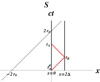
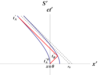
Fig. 4: Location-type experiment. World lines of the fixed observer and the object in $S$ transforms into hyperbolas in $S^{\prime}$. Thin lines are light signal world lines. Under the conformal transformations, light lines remain straight and inclined at $45^{\circ}$. In RF $S$ we have $t_{A}-t_{B}=t_{B}-t_{A}^{0}$, but in $S^{\prime}$ always the inequality $t^{\prime}_{A}-t^{\prime}_{B}>t^{\prime}_{B}-{t^{\prime}}_{\!A}^{0}$ takes place.

In application to real experiment analysis one should use (12) for the small time intervals, i.e., when $\Delta t/t_{lim}=(t_{A}-t_{A}^{0})/t_{lim}\ll 1$. In this case, formula (12) gives, to the second order of $t/t_{lim}$

$$t^{\prime}_{\pm}=t\mp\frac{t^{2}}{t_{lim}}.$$

In accordance with the location distance definition, the signal travelling distances in forward and backward directions, respectively, will be

$$x^{\prime}_{\pm}=ct^{\prime}_{\pm}=x\mp\Delta x=x\mp\frac{W_{0}}{2}t^{2},$$

where

$$W_{0}=\frac{2c}{t_{lim}}=2w.$$

Therefore in the $t/t_{lim}\ll 1$ approximation ($t$ is the signal propagation time) the forward and backward location distances $x^{\prime}_{\pm}$ differ from $R=ct$ by $\Delta x=\frac{W_{0}}{2}t^{2}$. From the usual point of view, it appears that the emitter fixed in any space point is subjected to constant acceleration $W_{0}=2w$ directed to the observer.

Clearly, $t/t_{lim}\ll 1$ condition is equivalent to the condition $\frac{wt}{2c}\ll 1$, $\frac{wx}{2c^{2}}\ll 1$ (see Sec. I), which formally corresponds to Galilei-Newton kinematics. So, the predicted effect in the location-type experiments will be the blue frequency shift, which value will be defined by the formula similar to (7), i.e.

$$\Delta\nu_{obs}=\nu_{0}\frac{W_{0}t}{c}.$$

Due to (28) the value of this shift is twice as large as predicted by (7).

For the constant rate of frequency shift $\dot{\nu}_{obs}=\frac{d(\Delta\nu_{obs})}{dt}$, we find the following relation analogous to (8):

$$\dot{\nu}_{obs}=\frac{1}{c}\nu_{0}W_{0}.$$

Since by (23) $W_{0}=cH_{0}$, where $H_{0}$ is the Hubble constant, from (30) we have

$$\dot{\nu}_{obs}=\nu_{0}H_{0}.$$

This relation defines the frequency drift as a function of the fixed emitter frequency $\nu_{0}$.

According to the approach under consideration the anomalous blue-shifted drift is the consequence of the non-inertiality of the observer’s RF. It can be observed in principle under suitable conditions (in the absence of any gravitating sources) on any frequency even in the case of mutually fixed emitter and receiver (see [9, 10, 11, 12]). From this point of view PA should be treated as the first clearly observed effect of that kind. The uniform blue-shifted drift $(\dot{\nu}_{obs})_{P}$ is measured experimentally with a great accuracy $(\dot{\nu}_{obs})_{P}=(5.99\pm 0.01)\cdot 10^{-9}$ Hz/s [3, 4]. Therefore it can form a basis for the new (alternative to the cosmological observations) high precision experimental estimation of the numerical value of the Hubble constant.

For that goal, we make use of (31), and recall that frequency of Pioneer tracking is $(\nu_{0})_{P}=2.29\cdot 10^{9}$ Hz, such that

$$H_{0}=\frac{(\dot{\nu}_{obs})_{P}}{(\nu_{obs})_{P}}\cong 2.62\cdot 10^{-18}\ \mbox{s}^{-1},$$

what is consistent with generally accepted value of $H_{0}\cong 2.4\cdot 10^{-18}\ \mbox{s}^{-1}$ obtained from cosmological observations.

For the ”acceleration” $a_{P}$ we have $a_{P}=cH_{0}=7.85\cdot 10^{-8}\ \mbox{cm/s}^{2},$ what is in the range of uncertainty of PA data ($a_{P}^{exp}=(8.74\pm 1.33)\cdot 10^{-8}$ cm/s²).

The numerical coincidence of the results can be considered as experimental evidence of anomalous blue-shifted drift as a kinematical manifestation of the conformal time inhomogeneity. In other words, from the view point of the considered approach, the quantities measured in experiments of electromagnetic wave propagation favor relation (29) (but not (7)) for the anomalous frequency shift.

It should be stressed that the physical meaning of the relations (7) and (29) is fundamentally different in spite of their visual similarity.

Equation (7), defining blue frequency shift by the non-inertiality of RF $S^{\prime}$, in fact was obtained in the Galilei-Newton kinematics. There time transformation under transition from RF $S$ to $S^{\prime}$ has the form $t=t^{\prime}$ (see (4)).

On the other side, formula (29) was obtained from the exact non-linear time transformation (12) defining the time inhomogeneity, that is, beyond the Galilei-Newton kinematics. “Constant acceleration” $W_{0}=2w$ appears due to the quadratic character of the first non-linear term in the power series expansion of $t^{\prime}(t)$ in terms of small parameter $t/t_{lim}$ in (12), while the location distance is defined as $R^{\prime}=ct^{\prime}$. Hence the “acceleration” $W_{0}$ is not a “truly” acceleration (i.e. its origin is not a force or a dynamical source) but rather a “mimic” acceleration.

The possibility of assigning the anomalous frequency drift observed in the signals transmitted by Pioneer 10/11 to the quadratic time inhomogeneity was noted in the first comprehensive works on PA [3] and [4]. However no theoretical reasons were mentioned for such a phenomenological approach.

On the other hand, the acceleration parameter $w=\frac{1}{2}cH_{0}$ seems to be a strictly natural candidate for the “minimal acceleration”, which is a fundamental dynamical parameter of the Modified Newton Dynamics (MOND) (see [13, 14]), which is a phenomenological alternative for the Cold Dark Matter approach.

Conclusions

The conformal time inhomogeneity leads to the following consequences:

• The cosmological location distance can be determined as an explicit function of red shift $R(z)$. The combination of this function with the SR expression for the longitudinal Doppler-effect $V(z)$ gives the explicit analytic expression for the ratio $V(z)/H_{0}R(z)$. The ratio coincides with the Hubble law in the limit of $z\ll 1$, and possesses a maximum at $z_{max}\simeq 0.475$. The appearance of this maximum is a pure kinematic manifestation of the time inhomogeneity and does not need any special gravitating sources (like the dark energy).

• In the location-type experiments uniform blue-shifted frequency drift appears, which mimics constant acceleration $w=cH_{0}$ directed towards the observer. The Pioneer Anomaly is the first really observed effect of that kind. The observed drift can be used for local experimental determination of Hubble constant. This effect can be observed in principle at any frequency even between mutually moveless emitter and receiver in the absence of any gravitating centers.

The topics discussed in the present report was considered in part in author’s papers [7, 8, 9, 10, 11, 12] as well.

References

- [1] A.G. Riess at al. Astron. J. 116, 1009(1998).
- [2] S. Perlmutter at al. Astrophys. J. 517, 565(1999).
- [3] J.D. Anderson et al. Phys. Rev. Lett. 81, 2858(1998); arXiv:gr-qc/9808081.
- [4] J.D. Anderson et al. Phys. Rev. D. 65, 082004(2002); arXiv:gr-qc/0104064.
- [5] M.M. Nieto, J.D. Anderson. ArXiv:gr-qc/0709.1917.
- [6] T. Fulton, F. Rohrlich and L. Witten. Nuovo Cim. 34, 652 (1962).
- [7] L.M. Tomilchik. ArXiv:gr-qc/0704.2745.
- [8] L.M. Tomilchik. Doklady of the National Academy of Sciences of Belarus. (to be published) (in Russian).
- [9] L.M. Tomilchik. ArXiv:gr-qc/0710.3994.
- [10] L.M. Tomilchik. Doklady of the National Academy of Sciences of Belarus. 50, N. 6, 51 (2007) (in Russian).
- [11] L.M. Tomilchik. Optics and Spectroscopy 103, 237 (2007) (in Russian); english version: 103, 218 (2007).
- [12] L.M. Tomilchik. Non-Euclidean Geometry in Modern Physics. Proc. 5th Int. Conf. Bolyai-Gauss-Lobachevsky (BGL-5), Minsk, 2006, p. 158–165.
- [13] M. Milgrom, Astrophys. J. 270, 365 (1983).
- [14] J. Bekenstein and M. Milgrom, Astrophys. J. 286, 7 (1984).