Ray-based calculations of backscatter in laser fusion targets

Abstract

A 1D, steady-state model for Brillouin and Raman backscatter from an inhomogeneous plasma is presented. The daughter plasma waves are treated in the strong damping limit, and have amplitudes given by the (linear) kinetic response to the ponderomotive drive. Pump depletion, inverse-bremsstrahlung damping, bremsstrahlung emission, Thomson scattering off density fluctuations, and whole-beam focusing are included. The numerical code deplete, which implements this model, is described. The model is compared with traditional linear gain calculations, as well as “plane-wave” simulations with the paraxial propagation code pf3d. Comparisons with Brillouin-scattering experiments at the OMEGA Laser Facility [T. R. Boehly et al., Opt. Commun. 133, p. 495 (1997)] show that laser speckles greatly enhance the reflectivity over the deplete results. An approximate upper bound on this enhancement, motivated by phase conjugation, is given by doubling the deplete coupling coefficient. Analysis with deplete of an ignition design for the National Ignition Facility (NIF) [J. A. Paisner, E. M. Campbell, and W. J. Hogan, Fusion Technol. 26, p. 755 (1994)], with a peak radiation temperature of 285 eV, shows encouragingly low reflectivity. Re-absorption of Raman light is seen to be significant in this design.

I Introduction

Laser-plasma interaction (LPI) Kruer (2003) is an important plasma-physics problem which poses serious challenges to theoretical modeling. LPI is the basis of several applications, including laser-based particle acceleration Tajima and Dawson (1979) and the backward Raman amplifier Malkin et al. (1999). Moreover, for inertial confinement fusion (ICF)Atzeni and ter Vehn (2004); Lindl et al. (2004) to succeed, LPI must not be so active that it prevents the desired laser energy from being delivered to the target, with the desired spatial and temporal behavior. This paper focuses on modeling the backscatter instabilities, where a laser light wave (mode 0) decays into a backscattered light wave (mode 1) and a plasma wave (mode 2). In stimulated Raman scattering (SRS) and stimulated Brillouin scattering (SBS), the plasma wave is, respectively, an electron plasma wave and an ion acoustic wave. These LPI processes pose a serious risk to indirect-drive ICF Lindl et al. (2004).

A wide array of computational tools is used to model LPI, ranging from rapid ($\sim$secs) calculations of linear gains along 1D profiles to massively-parallel kinetic particle-in-cell simulations. We present here a new tool, called deplete, to the less computationally expensive end of this spectrum. deplete solves for the pump intensity and scattered-wave spectral density for a set of scattered frequencies, in steady-state, along a 1D profile of plasma conditions. Pump depletion is included, and the plasma waves are assumed to be in the strong damping limit (i.e., they do not advect). Fully kinetic (although linear) formulas are used for various quantities like the coupling coefficient. Bremsstrahlung noise and damping, as well as Thomson scattering (TS), are included. The deplete model, especially the noise sources, in some ways resembles that of Ref. Berger et al. (1989). Other similar works which have influenced our thinking, and use 1D coupled-mode equations, are Refs. Ramani and Max (1983)-Mounaix et al. (1997).

deplete is a 1D model, but the plasma conditions are generally found by tracing 3D geometric-optics ray paths through the output of a radiation-hydrodynamics code. We therefore call this combined approach to studying LPI a ray-based one. Details of this methodology, and its limits, are discussed in Sec. III.

deplete is similar to the code newlip, which calculates linear gains for SRS and SBS along 1D profiles (newlip is discussed here in Appendix A). Both codes take seconds to analyze one profile from the laser entrance to the high-Z wall in an ICF ignition design. However, deplete includes substantially more physics than newlip, such as pump depletion, noise sources, and re-absorption of scattered light. deplete moreover provides pump and scattered intensities, which unlike gains can be directly compared with experiment and more sophisticated LPI codes. Despite its simplicity, deplete agrees well in certain cases with results from the 3D paraxial laser propagation code pf3d. This is quite promising given deplete’s much lower computing cost.

There is important physics which deplete does not capture, with laser speckles or hot spots being one of the most important. Recent SBS experiments Froula et al. (2007a); Neumayer et al. (2008) at the OMEGA Laser Facility Boehly et al. (1997) show good agreement between measured reflectivity and pf3d predictions, while deplete gives a lower value. This is due to the speckle pattern of the phase plate smoothed lasers. Sec. VIII describes one approximate way to bound the speckle enhancement by doubling the coupling coefficient; the resulting deplete reflectivity always exceeds the experimental level. A more sophisticated idea for handling speckles is outlined in the conclusion. Additional beam smoothing, like polarization smoothing (PS) and smoothing by spectral dispersion (SSD), reduce the effective speckle intensity and can reduce the reflectivity even below the speckle-free deplete level.

The paper is organized as follows. Section II derives the governing equations for the pump intensity and scattered-wave spectral density. Our ray-based methodology and model limits are discussed in Sec. III. The numerical method is given in Sec. IV, including a quasi-analytic solution for the coupling-Thomson step. Section V compares deplete with newlip linear gains and pf3d “plane-wave” simulations on prescribed profiles. The relationship between Thomson scattering and linear gain is discussed in Sec. VI. In Sec. VII we compare deplete to the experimental and pf3d SBS reflectivities in recent OMEGA shots. Sec. VIII presents deplete analysis of an ignition design with a 285 eV radiation temperature for the National Ignition Facility (NIF) Paisner et al. (1994). In particular, we show the effect of scattered light re-absorption and put a bound on speckle enhancement. We conclude and discuss future prospects in Sec. IX. A review of newlip and its linear gain is presented in Appendix A. Appendix B details the numerics of deplete’s coupling-Thomson step.

II Governing equations

We derive coupled-mode equations, in time and one space dimension, for the slowly-varying wave envelopes, and find the resulting intensity equations. We do this for the light waves first, and then the plasma wave in the strong damping limit. Since our approach is standard we summarize some steps. We take these equations in steady state to apply independently at each scattered frequency, and transition to a spectrum of scattered light per angular frequency. This may be viewed as a “completely incoherent” treatment of the scattered light at different frequencies. Bremsstrahlung damping and fluctuations, and TS, are then added phenomenologically. Focusing of the whole beam is finally accounted for, giving the system deplete solves. This section culminates in the deplete system, Eqs. (54-55), on which some readers may wish to focus.

II.1 light-wave action equations

Let $z$ be distance along the profile, and assume all wave vectors and gradients are in $z$ ($\partial_{x}=\partial_{y}=0$). $z=0$ is taken as the left edge of the domain (the “laser entrance”), where we specify the right-moving pump laser; we also specify boundary values for the left-moving backscattered wave at the right edge $z=L_{z}$. The light waves are linearly polarized in $y$ and represented by their vector potentials $\vec{A}_{i}=(1/2)A_{i}(z,t)\hat{y}e^{i\psi_{i}}+cc$, where $i=0,1$ for the pump and scattered wave, respectively. $A_{i}$ is the slowly-varying complex envelope, and we use the dimensionless $a_{i}\equiv eA_{i}/m_{e}c$. $\psi_{i}(z,t)$ is the rapidly-varying phase with $k_{i}\equiv\partial_{z}\psi_{i}$ and $\omega_{i}\equiv-\partial_{t}\psi_{i}$. Let $\sigma_{i}\equiv k_{i}/|k_{i}|$ with $\sigma_{0}=\sigma_{2}=+1$ and $\sigma_{1}=-1$ (appropriate for backscatter). Thermal fluctuations give rise to both light waves and plasma waves. However, upon appropriate averaging the field amplitudes of these fluctuations vanish (but their mean squares do not). The amplitudes $A_{i}$ (and $n_{j2}$ below) represent only the coherent, and not the noise, components of the fields. We insert a bremsstrahlung noise source and TS to the intensity equations below.

From the Maxwell equations, and conservation of canonical transverse momentum $m_{e}v_{ye}=eA_{y}$, we find $A_{y}=(\vec{A}_{0}+\vec{A}_{1})\cdot\hat{y}$ satisfies

$$\left[\partial_{tt}-c^{2}\partial_{zz}+\omega_{pe}^{2}\right]A_{y}=-\omega_{pe}^{2}{n_{e2}\over n_{e}}A_{y}.$$ (1)

$\tilde{n}_{j}=n_{j}+N_{j2}$ is the total number density for species $j$ ($j=e$ for electrons, $i$ for an ion species), $N_{j2}=(1/2)n_{j2}e^{i\psi_{2}}+cc$, and $n_{j2}$ is the slowly-varying plasma-wave envelope. We define $\omega_{pj}\equiv[n_{j}Z_{j}^{2}e^{2}/\epsilon_{0}m_{j}]^{1/2}$, $v_{Tj}\equiv[T_{j}/m_{j}]^{1/2}$ and $\lambda_{Dj}\equiv v_{Tj}/\omega_{pj}$, with $Z_{j}$ the charge state. As usual, the massive ions are treated as fixed in the transverse current. (We look forward to a circumstance where a positively-charged species must be considered mobile, such as an electron-positron plasma!)

Following, e.g., Ref. Dewandre et al. (1981), we introduce the small parameter $\delta\sim\omega_{i}^{-1}\partial_{t}\ln X\sim k_{i}^{-1}\partial_{x}\ln X$ for $X=A_{i},k_{i},$ etc. We order $\partial_{t},\partial_{x}\sim\delta$, $\psi_{i}\sim\delta^{-1}$, and the right-hand side of Eq. (1) $\sim\delta$. To order $\delta^{0}$, we obtain the free-wave dispersion relation

$$\omega_{i}^{2}=\omega_{pe}^{2}+c^{2}k_{i}^{2}\qquad i=0,1.$$ (2)

For the steady-state conditions considered below we take $\omega_{i}$ to be constant and find the eikonal $ck_{i}(x)=\sigma_{i}\eta_{i}\omega_{i}$ with $\eta_{i}\equiv[1-n_{e}/n_{ci}]^{1/2}$ and $n_{ci}\equiv\omega_{i}^{2}\epsilon_{0}m_{e}/e^{2}$ the critical density of mode $i$. Also, the group velocity is $v_{gi}\equiv\sigma_{i}\eta_{i}c$.

Assuming perfect phase matching ($k_{0}=k_{1}+k_{2}$, $\omega_{0}=\omega_{1}+\omega_{2}$), the resonant order $\delta$ terms in Eq. (1) yield the envelope equations:

$$L_{0}a_{0} = -{i\over 4}{\omega_{pe}^{2}\over\omega_{0}}{n_{e2}\over n_{e}}a_{1},$$ (3)

$$L_{0}a_{1} = -{i\over 4}{\omega_{pe}^{2}\over\omega_{1}}{n_{e2}^{*}\over n_{e}}a_{0}.$$ (4)

The operator $L_{i}\equiv\partial_{t}+v_{gi}\partial_{z}+(1/2\omega_{i})(\partial_{t}\omega_{i}+c^{2}\partial_{z}k_{i})$. Our quasi-monochromatic light waves ($i=0,1$) have action density Bers (1975) $N_{i}\equiv(m_{e}/8\pi r_{e})\omega_{i}a_{i}a_{i}^{*}$ where $r_{e}\equiv e^{2}/4\pi\epsilon_{0}m_{e}c^{2}\approx 2.82$ fm. We also define the (positive) action flux $Z_{i}\equiv N_{i}|v_{gi}|$ and intensity $I_{i}\equiv\omega_{i}Z_{i}$. In practical units,

$$|a_{i}|^{2}={I_{i}\lambda_{i}^{2}\over P_{em}\eta_{i}}$$ (5)

where $\lambda_{i}\equiv 2\pi c/\omega_{i}$ and $P_{em}\equiv(\pi/2)m_{e}c^{3}/r_{e}$ $\approx 1.37\times 10^{18}$ W$\cdot$cm${}^{-2}\cdot\mu$m². We form Eq. (3)$\times a_{0}^{*}+cc$ and Eq. (4)$\times a_{1}^{*}+cc$ to find

$$-\partial_{t}N_{0}-\partial_{z}Z_{0} = \partial_{t}N_{1}-\partial_{z}Z_{1}=J$$ (6)

$$J \equiv -{1\over 4}m_{e}c^{2}\ \mathrm{Im}[a_{0}^{*}a_{1}n_{e2}].$$ (7)

II.2 plasma-wave action equations

We describe the plasma waves following the dielectric operator approach of Cohen and Kaufman Cohen and Kaufman (1977):

$$\epsilon(\omega_{2}^{\prime}+i\partial_{t},k_{2}-i\partial_{z})n_{2}\ = n_{\mathrm{pnd}},$$ (8)

$$n_{\mathrm{pnd}} \equiv \chi_{e}(\omega_{2}^{\prime},k_{2}){c^{2}k_{2}^{2}\over 2\omega_{pe}^{2}}n_{e}a_{0}a_{1}^{*}.$$ (9)

The charge-density fluctuation $n_{2}\equiv-n_{e2}+\sum_{i}Z_{i}n_{i2}$ experiences a ponderomotive drive $n_{\mathrm{pnd}}$. $\omega_{2}^{\prime}\equiv\omega_{2}-\vec{k}_{2}\cdot\vec{u}$ is the Doppler-shifted plasma-wave frequency in the frame of the plasma flow $\vec{u}$ ($\omega_{2}$ is in the lab frame). $\epsilon\equiv 1+\chi$ is an operator, where the time and space derivatives reflect envelope evolution and $\chi\equiv\sum_{j}\chi_{j}$ is the total susceptibility. $\chi_{e}$ in $n_{\mathrm{pnd}}$ is simply a function, not an operator. $\chi_{j}$ is the (linear) kinetic, collisionless susceptibility of Maxwellian species $j$:

$$\chi_{j}\equiv-{1\over 2k_{2}^{2}\lambda_{Dj}^{2}}Z^{\prime}(\zeta_{j});\qquad\zeta_{j}\equiv{\omega_{2}^{\prime}\over k_{2}v_{Tj}\sqrt{2}}.$$ (10)

$Z(\zeta)\equiv i\pi^{1/2}e^{-\zeta^{2}}\mathrm{erfc}(-i\zeta)$ is the plasma dispersion function Fried and Conte (1961) and $\mathrm{erfc}$ is the complimentary error function Abramowitz and Stegun (1970). Gauss’s law relates $n_{2}$ and $n_{j2}$:

$$n_{e2} = -(1+\chi_{I})n_{2},$$ (11)

$$n_{i2} = -\chi_{i}\left({1\over Z_{i}}+{m_{e}\over m_{i}}{\epsilon\over\chi_{e}}\right)n_{2}$$ (12)

$$\approx -{\chi_{i}\over Z_{i}}n_{2},$$ (13)

with $\chi_{I}\equiv\sum_{i}\chi_{i}$. For SRS, where the ion motion is negligible, we usually take $1+\chi_{I}\rightarrow 1$ to save computing time.

Expanding $\epsilon$ for slow envelope variation, and retaining only $\epsilon_{r}\equiv\mathrm{Re}\,\epsilon$ in the derivatives, gives

$$\left[\partial_{t}+v_{g2}\partial_{z}+\nu_{2}+i\delta\omega_{2}\right]n_{2}=-i{n_{\mathrm{pnd}}\over\dot{\epsilon}}.$$ (14)

$\dot{\epsilon}\equiv\partial\epsilon_{r}/\partial\omega_{2}^{\prime}$, $\epsilon^{\prime}\equiv\partial\epsilon_{r}/\partial k_{2}$, $v_{g2}\equiv-\epsilon^{\prime}/\dot{\epsilon}$ is the plasma-wave group velocity, $\nu_{2}\equiv\mathrm{Im}[\epsilon]/\dot{\epsilon}$ is the damping rate, and $\delta\omega_{2}\equiv-\epsilon_{r}/\dot{\epsilon}$ is the phase detuning.

We now assume the plasma wave is in the strong damping limit, where its advection is neglected: $|v_{g2}\partial_{z}n_{2}|\ll|\nu_{2}+i\delta\omega_{2}||n_{2}|$. This implies the instability is below its absolute threshold so that steady-state solutions are accessible. Also going to steady-state, we find

$$\epsilon(\omega_{2},k_{2})n_{2}=n_{\mathrm{pnd}}.$$ (15)

Replacing $n_{e2}$ via Eqs. (11) and (15) yields

$$J=\omega_{0}\tilde{\Gamma}_{1}Z_{0}Z_{1}.$$ (16)

The coupling coefficient $\tilde{\Gamma}_{1}$ is

$$\tilde{\Gamma}_{1} \equiv \Gamma_{S}\mathrm{Im}\left[{\chi_{e}\over\epsilon}(1+\chi_{I})\right]={\Gamma_{S}g_{\Gamma}\over|\epsilon|^{2}},$$ (17)

$$\Gamma_{S} \equiv {2\pi r_{e}\over m_{e}c^{2}}{1\over\omega_{0}}{k_{2}^{2}\over k_{0}|k_{1}|},$$ (18)

$$g_{\Gamma} \equiv |1+\chi_{I}|^{2}\mathrm{Im}\chi_{e}+|\chi_{e}|^{2}\mathrm{Im}\chi_{I}.$$ (19)

The second form of $\tilde{\Gamma}_{1}$ exhibits the resonance for $|\epsilon|\ll 1$. The over-tilde on $\tilde{\Gamma}_{1}$ indicates it will be modified below to account for beam focusing. $\tilde{\Gamma}_{1}$, and thus $J$, are usually positive. We now have a closed system for modes 0 and 1, with no independent equation for mode 2:

$$\partial_{t}N_{0}+\partial_{z}Z_{0} = -\omega_{0}\tilde{\Gamma}_{1}Z_{0}Z_{1},$$ (20)

$$\partial_{t}N_{1}-\partial_{z}Z_{1} = \omega_{0}\tilde{\Gamma}_{1}Z_{0}Z_{1}.$$ (21)

II.3 Steady-state equations for a spectrum of scattered waves

We transition to steady state ($\partial_{t}=0$) and work with intensities. Since we have assumed $\partial_{z}\omega_{i}=0$, we multiply Eq. (20) by $\omega_{0}$ and Eq. (21) by $\omega_{1}$ to obtain

$$d_{z}I_{0} = -{\omega_{0}\over\omega_{1}}\tilde{\Gamma}_{1}I_{0}I_{1},$$ (22)

$$-d_{z}I_{1} = \tilde{\Gamma}_{1}I_{0}I_{1}.$$ (23)

Here and elsewhere, $d_{x}f(x)$ denotes the ordinary derivative of a function of one variable, while $\partial_{x}f$ denotes the partial derivative of a function of several variables.

The bremsstrahlung source and TS are expressed in terms of spectral density $i_{1}(z,\omega_{1})$ (intensity per angular frequency). The scattered intensity is then $I_{1}=\int d\omega_{1}\,i_{1}$. We take Eq. (23) to apply independently at each $\omega_{1}$, and integrate the coupling term in Eq. (22), to find

$$d_{z}I_{0} = -\int d\omega_{1}{\omega_{0}\over\omega_{1}}\tilde{\Gamma}_{1}I_{0}i_{1},$$ (24)

$$-\partial_{z}i_{1} = \tilde{\Gamma}_{1}I_{0}i_{1}.$$ (25)

This is a totally incoherent treatment of the scattered light at different frequencies, and is unrealistic to the extent there is spectral “leakage” between nearby $\omega_{1}$ intervals due to, e.g., envelope evolution.

II.4 Bremsstrahlung source and damping

We incorporate electron-ion inverse-bremsstrahlung light-wave damping ($\kappa_{0}$ and $\kappa_{1}$) phenomenologically for modes 0 and 1, as well as bremsstrahlung noise ($\tilde{\Sigma}_{1}$) for mode 1, to find

$$d_{z}I_{0} = -\kappa_{0}I_{0}-\int d\omega_{1}{\omega_{0}\over\omega_{1}}\tilde{\Gamma}_{1}I_{0}i_{1},$$ (26)

$$-\partial_{z}i_{1} = -\kappa_{1}i_{1}+\tilde{\Sigma}_{1}+\tilde{\Gamma}_{1}I_{0}i_{1}.$$ (27)

As for $\tilde{\Gamma}_{1}$, the over-tilde on $\tilde{\Sigma}_{1}$ denotes it will be modified due to focusing.

$I_{0}$ and $i_{1}$ represent integrals over solid angles in $k$ space, which we now specify. Absolute solid angles are needed in the noise sources, and cannot be simply scaled away, because scattered intensities determine pump depletion. We follow closely Bekefi’s book Bekefi (1966) in this section. We take $I_{i}=\Omega_{i}I_{i,\Omega}$ for $i=0,1$ (see Secs. 1.6 and 1.7 of Bekefi). $I_{i,\Omega}$ is the intensity per solid angle interval $d\Omega$ in $k$ space, which we assume is constant over the solid angle $\Omega_{i}$ that participates in the scattering. $\Omega_{i}$ is the local (in $z$) solid angle in the plasma, which we express in terms of a cone half-angle $\theta_{p,i}$ as

$$\Omega_{i}\equiv 2\pi(1-\cos\theta_{p,i}).$$ (28)

From Snell’s law, $\theta_{p,i}$ varies with $z$ according to

$$\cos\theta_{p,i}=\begin{cases}0\quad\mathrm{if}\ n_{e}\geq n_{ci}\cos^{2}\theta_{v}\\ [1-\eta_{i}^{-2}\sin^{2}\theta_{v}]^{1/2}\quad\mathrm{otherwise}.\end{cases}$$ (29)

$n_{ci}\cos^{2}\theta_{v}$ is the “critical density” above which we cut off backscatter ($\tilde{\Gamma}_{1}=\tilde{\Sigma}_{1}=\kappa_{1}=0$). $\theta_{v}$ is a “vacuum” cone angle, which we find from the solid angle in the beam’s F-cone (for simplicity we use the same solid angle for pump and scattered light). This is reasonable if the scattering mostly occurs in laser speckles that are near diffraction-limited. In terms of laser optics F-number $F$,

$$\cos\theta_{v} \equiv \left[1+{1\over 4F^{2}}\right]^{-1/2}\approx 1-{1\over 8F^{2}},$$ (30)

$$\Omega_{i}^{v} \equiv 2\pi(1-\cos\theta_{v})\approx{\pi\over 4F^{2}}.$$ (31)

The approximate forms apply for $F\gg 1$.

The upshot of the solid angle discussion (see especially Eq. (1.133) of Bekefi) is

$$\tilde{\Sigma}_{1}=\Omega_{1}j(\omega_{1}),$$ (32)

where $j(\omega)$ is the emission coefficient, per $d\Omega$ and in one polarization (see p. 134 of Bekefi):

$$j(\omega_{i})={\eta_{i}\over 12\pi^{3}\sqrt{2\pi}}{\omega_{pe}^{4}\over v_{Te}}{m_{e}r_{e}\over c}\sum_{j\in\mathrm{ions}}{n_{j}\over n_{e}}Z_{j}^{2}\ln\Lambda_{ej}.$$ (33)

$\ln\Lambda_{ej}$ is sometimes called the Gaunt factor and resembles the Coulomb logarithm, although it arises in calculations without ad hoc cutoffs on impact parameter integrals (see Chap. 3 of Bekefi). For the case $\omega_{i}>\omega_{pe}$, Bekefi finds $\Lambda_{ej}=v_{Te}/(\omega_{i}b_{\mathrm{min}})$ where

$$b_{\mathrm{min}}=\begin{cases}{\gamma\over 4}{\hbar\over\sqrt{m_{e}T_{e}}}&\mathrm{if}\ T_{e}>77Z_{j}^{2}\ \mathrm{eV},\\ \left({\gamma\over 2}\right)^{5/2}Z_{j}r_{e}{m_{e}c^{2}\over T_{e}}&\mathrm{otherwise}.\end{cases}$$ (34)

The first, high-$T_{e}$ case typically applies for hohlraum conditions. The numerical pre-factors come from a detailed binary-collision calculation, and $\gamma=e^{C}\approx 1.781$ where $C\approx 0.577$ is the Euler-–Mascheroni constant. Our expression for $j$ does not include the enhanced emission for $\omega_{i}\approx\omega_{pe}$ due to collective effects Dawson and Oberman (1962).

We find the absorption coefficient $\kappa_{i}$ via Kirchoff’s law (see Bekefi Sec. 2.3):

$$\kappa_{i}={\Omega_{i}\over\Omega_{i}^{v}}{j(\omega_{i})\over B_{v}(\omega_{i})}.$$ (35)

Our $\kappa_{i}$ equals Bekefi’s $\alpha_{\omega}$. $B_{v}$ is the vacuum blackbody spectrum for one polarization, with units $dI/(d\omega\,d\Omega)$:

$$B_{v}(\omega) \equiv {\hbar\over 8\pi^{3}c^{2}}{\omega^{3}\over e^{\hbar\omega/T_{e}}-1}$$ (36)

$$\approx {\omega^{2}T_{e}\over 8\pi^{3}c^{2}}\qquad\hbar\omega\ll T_{e}.$$ (37)

$j$ given above was found for collision durations short compared to the light-wave period, which entails the Jeans limit $\hbar\omega\ll T_{e}$. We therefore use the approximate form of $B_{v}$ to obtain

$$\kappa_{i}={\sqrt{2}\over 3\sqrt{\pi}}{\Omega_{i}\over\Omega_{i}^{v}}{r_{e}c\eta_{i}\over\omega_{i}^{2}}{\omega_{pe}^{4}\over v_{Te}^{3}}\sum_{j\in\mathrm{ions}}{n_{j}\over n_{e}}Z_{j}^{2}\ln\Lambda_{ej}.$$ (38)

For an optically thick plasma ($\partial_{z}i_{1}=0$) with no pump ($I_{0}=0$), we obtain for $i_{1}$ from Eq. (27) the fluctuation level $i_{1}^{\mathrm{OT}}$:

$$i_{1}^{\mathrm{OT}}\equiv{\Sigma_{1}\over\kappa_{1}}={\Omega_{1}^{v}\over f}B_{v}(\omega_{1}).$$ (39)

$f$ and $\Sigma_{1}$ are defined in Sec. II.6. We thus recover the blackbody spectrum, required by Kirchoff’s law. The factor $\eta_{1}^{2}$ that usually appears in the blackbody spectrum in a plasma is absent due to our treatment of solid angles.

II.5 Thomson scattering

Thomson scattering (TS) refers to scattering off plasma-wave fluctuations resulting from particle discreteness (Oberman and Williams (1983), p. 308). Had we retained a separate plasma wave equation, the fluctuations would appear in it as Čerenkov emission Berger et al. (1989). It is an important noise source for backscatter, especially for SBS. We express $\Delta p_{1}$, the TS scattered power increment per $d\omega_{1}$ per $d\Omega_{1}$ ($k_{1}$ solid angle), within a thin slab of width $\Delta z$, as

$$\Delta p_{1} = {d\sigma\over d\omega_{1}d\Omega_{1}}I_{0}$$ (40)

$${d\sigma\over d\omega_{1}d\Omega_{1}} = n_{e}A(z)\Delta z\psi r_{e}^{2}{S\over 2\pi}.$$ (41)

$A(z)$ is the beam area, defined in Sec. II.6. $\psi\equiv 1-\sin^{2}\theta_{s}\sin^{2}\theta_{a}$ is a geometric factor. $\theta_{s}$ is the angle between $\vec{k}_{0}$ and $\vec{R}$, the vector from source to “observation point”. For a beam with large $F$, $\theta_{s}\sim\theta_{v}\ll 1$. $\theta_{a}$ is the angle between $\vec{R}$ and the pump polarization. We usually take $\psi=1$.

The form factor $S$ (units of time) is from Eq. (138) of Ref. Oberman and Williams (1983), valid for arbitrary (non-Maxwellian) distributions, generalized to multiple ion species:

$${|\epsilon|^{2}\over 2\pi}S(\vec{k},\omega) = |1+\chi_{I}|^{2}F_{e}+|\chi_{e}|^{2}\sum_{j\in\mathrm{ions}}{n_{j}\over n_{e}}Z_{j}^{2}F_{j}$$ (42)

$$F_{j} \equiv \int d^{3}v\ f_{j}(\vec{v})\delta(\omega+\vec{k}\cdot\vec{v}).$$ (43)

$f_{j}$ is the distribution function of species $j$ $(\int d^{3}v\ f_{j}=1)$. For a Maxwellian,

$$F_{j}={1\over kv_{Tj}\sqrt{2\pi}}e^{-\zeta_{j}^{2}}={(k\lambda_{Dj})^{2}\over\pi\omega}\mathrm{Im}\chi_{j},$$ (44)

and

$${\omega|\epsilon|^{2}\over 2(k\lambda_{De})^{2}}S=g_{\tau}\equiv|1+\chi_{I}|^{2}\mathrm{Im}\chi_{e}+|\chi_{e}|^{2}\sum_{j\in\mathrm{ions}}{T_{j}\over T_{e}}\mathrm{Im}\chi_{j}.$$ (45)

This form agrees with the multiple-ion result in Eq. (3) of Ref. Evans (1970). Henceforth we assume Maxwellian distributions.

From Eq. (40) we form a differential equation for $i_{1}$ that describes TS:

$$\left.\partial_{z}i_{1}\right|_{TS}=\tau_{1}I_{0}\qquad\tau_{1}\equiv{\Omega_{1}\over AI_{0}}{\Delta p_{1}\over\Delta z}.$$ (46)

Since TS transfers energy from the pump to the scattered waves, we include it in both equations:

$$d_{z}I_{0} = -\kappa_{0}I_{0}-\int d\omega_{1}{\omega_{0}\over\omega_{1}}I_{0}(\tau_{1}+\tilde{\Gamma}_{1}i_{1}),$$ (47)

$$-\partial_{z}i_{1} = -\kappa_{1}i_{1}+\tilde{\Sigma}_{1}+I_{0}(\tau_{1}+\tilde{\Gamma}_{1}i_{1}).$$ (48)

For conevience we write $\tau_{1}$ as

$$\tau_{1} = \Omega_{1}n_{e}r_{e}^{2}\psi{S(k_{2},\omega_{2}^{\prime})\over 2\pi}={\tau_{S}g_{\tau}\over|\epsilon|^{2}},$$ (49)

$$\tau_{S} \equiv {\Omega_{1}\psi\over\pi}n_{e}r_{e}^{2}{(k_{2}\lambda_{De})^{2}\over\omega_{2}^{\prime}}.$$ (50)

$\tau_{1}$ is always positive, while $\tau_{S}$ and $g_{\tau}$ have the same sign as $\omega_{2}^{\prime}$ (which can be negative for IAW’s when the plasma flow is supersonic along $\vec{k}_{0}$).

It is useful to note that $i_{\tau}\equiv\tau_{1}/\Gamma_{1}$ sometimes plays the role of an effective seed level for $i_{1}$:

$$i_{\tau}\equiv{\tau_{1}\over\Gamma_{1}}={\tau_{S}g_{\tau}\over\Gamma_{S}g_{\Gamma}}.$$ (51)

For the special case $T_{i}=T_{e}$, we have $g_{\tau}=g_{\Gamma}$ and $i_{\tau}$ is independent of $\chi_{j}$:

$$i_{\tau}={\tau_{S}\over\Gamma_{S}}={\Omega_{1}\psi\over(2\pi)^{3}}{\omega_{0}\over\omega_{2}^{\prime}}T_{e}k_{0}|k_{1}|,\qquad T_{i}=T_{e}.$$ (52)

This fact is used in Sec. VI to discuss the relation of TS to linear gain.

II.6 Whole-beam focusing

We wish to incorporate the effects of whole-beam focusing in a simple way. The equations as written hold locally in $z$, but do not model focusing. To do this, we treat the transverse intensity patterns of $I_{0}$ and $I_{1}$ to be uniform flattops of varying area $A(z)$. The beam focuses at the focal spot $z_{F}$, where $A$ attains its minimum $A(z_{F})$. Let $\tilde{I}_{i}\equiv I_{i}(z)/f(z)$ be the total power at $z$ divided by the focal spot area, with focusing factor $f\equiv A(z_{F})/A(z)\leq 1$. We typically employ for $f$ the result for the on-axis intensity of a gaussian beam Milonni and Eberly (1988):

$$f=[1+(z-z_{F})^{2}/z_{0}^{2}]^{-1}$$ (53)

where $z_{0}$ is an effective Rayleigh range. For a Gaussian beam with optics F-number $F$, $z_{0}=(4/\pi)\lambda F^{2}$. This form approximately fits the random phase plate (RPP) smoothed beams designed for NIF (for an appropriate $z_{0}$).

Substituting $(I_{0},i_{1})=f\cdot(\tilde{I}_{0},\tilde{i}_{1})$ into Eqs. (47-48), and freely commuting $f$ with $\partial_{z}$, yields the principal equations solved by deplete:

$$d_{z}I_{0}(z) = -\kappa_{0}I_{0}-I_{0}\int d\omega_{1}\ {\omega_{0}\over\omega_{1}}(\tau_{1}+\Gamma_{1}i_{1}),$$ (54)

$$\partial_{z}i_{1}(z,\omega_{1}) = \kappa_{1}i_{1}-\Sigma_{1}-I_{0}(\tau_{1}+\Gamma_{1}i_{1}).$$ (55)

$\Gamma_{1}\equiv f\tilde{\Gamma}_{1}$ and $\Sigma_{1}\equiv f^{-1}\tilde{\Sigma}_{1}.$ In Eqs. (54-55) and henceforth, all $I_{i}$ and $i_{1}$ are understood to have suppressed over-tildes, that is, to refer to total transverse powers over focal-spot area. Similarly, the plasma-wave amplitude from Eq. (15) can be written

$${n_{2}\over n_{e}}={1\over 2}{\chi_{e}\over\epsilon}\left[{ck_{2}\over\omega_{pe}}\right]^{2}f\ \tilde{a}_{0}\tilde{a}_{1}^{*}$$ (56)

with $\tilde{a}_{i}^{2}\equiv\tilde{I}_{i}\lambda_{i}^{2}/(P_{em}\eta_{i})$; see Eq. (5).

All symbols in Eqs. (54-55) are positive, except $\Gamma_{1}$ may be negative for SBS in case $\omega_{2}^{\prime}<0$. This corresponds to the scattered wave having a higher frequency than the pump, in the plasma frame. The scattered wave then gives energy to the pump, and deplete handles this situation correctly.

III Ray methodology and model limits

deplete calculates LPI along given plasma conditions for a 1D profile. A typical application is to study a laser beam propagating through conditions given by a rad-hydro simulation. We use many independent rays to model the whole beam, which introduces some statistical inaccuracy. The rays are generally found by tracing 3D refracted paths through the rad-hydro output. Although strictly not a part of deplete, this is the major way we utilize geometric-optics rays. Wave-optics effects, such as laser speckles and diffraction (of both the pump and scattered light), are also not included in deplete. We present one way to approximate gain enhanacement due to speckles in Sec. VII.

However, laser intensity is not found from a rad-hydro simulation. Such codes generally treat a laser beam as a set of rays, which are absorbed as they trace out refracted paths. The laser intensity in a zone is found by dividing the total power of all rays crossing that zone by its transverse area. This approach suffers from several problems for our purposes, including the fact that intensities remain finite at caustics only due to the finite number of rays and zone size. Instead, we run deplete separately for each ray, and use a model for the laser beam to give an initial intensity (at a sufficiently low density that little absorption has occurred) and $z$-dependent focusing factor (generally based on vacuum propagation). The intensity along a deplete 1D profile is thus independent of refraction that occurs due to the plasma. Refractive changes in beam intensity occur, for instance, when a beam propagates between two high-density regions. However, our independent-ray treatment has the benefit that caustics pose no problem.

deplete assumes that the laser and scattered light follow the same path, and thus see the same plasma conditions. The two light waves refract differently if their wavelengths differ, as in SRS, or in SBS for certain transverse plasma flows Hinkel et al. (1999). The departure of ray paths becomes significant when the two rays see sufficiently different plasma conditions in the gain region for a given wavelength that the coupling or other coefficients differ significantly. This requires sufficiently strong transverse plasma gradients.

IV Numerical method

We solve the deplete system Eqs. (54-55) from the laser entrance $z=0$ to the right edge $z=L_{z}$. For backscatter (considered in this paper), we give $I_{0L}$ and $i_{1R}(\omega_{1})$ as boundary conditions, where $f_{L}\equiv f(z=0)$ and $f_{R}\equiv f(z=L_{z})$. We solve this two-point boundary value problem via a shooting method, marching from right to left. We guess $I_{0R}$ and solve the initial value problem from $z=L_{z}$ down to $z=0$, and iterate until the resulting $I_{0L}$ is sufficiently close to the desired value. Because $I_{0R}$ is just one scalar, it is more feasible to shoot on it than on the set of values $i_{1L}(\omega_{1})$. Generalizing our approach to 3D, where one would have to shoot on $I_{0R}(x,y)$ over a transverse plane, is much more difficult; a different technique for 3D pump depletion is used in the code slip Froula et al. (2008). For the right-boundary seed value $i_{1R}$, we either use 0 or the optically-thick $i_{1}^{\mathrm{OT}}$ from Eq. (39). The choice seems to have little effect, since volume sources (either TS or bremsstrahlung) typically produce a comparable or larger noise level after a short distance.

We solve Eqs. (54-55) by operator splitting Strang (1968); Yanencko (1970). Let the operator $B$ solve the “bremsstrahlung” system

$$d_{z}I_{0} = -\kappa_{0}I_{0},$$ (57)

$$\partial_{z}i_{1} = \kappa_{1}i_{1}-\Sigma_{1},$$ (58)

and the operator $C$ solve the “coupling-Thomson” system

$$d_{z}I_{0} = -I_{0}\int d\omega_{1}\ {\omega_{0}\over\omega_{1}}(\tau_{1}+\Gamma_{1}i_{1}),$$ (59)

$$\partial_{z}i_{1} = -I_{0}(\tau_{1}+\Gamma_{1}i_{1}).$$ (60)

To advance the solution from the discrete gridpoint $z^{n}$ down to $z^{n-1}$ (the decreasing index matches deplete’s right-to-left marching), we first apply $B$ for a half-step, then $C$ for a full step, then $B$ for a half-step again. The splitting theorem guarantees that if $B$ and $C$ are second-order accurate operators, then the overall step is second-order accurate. Schematically, a complete step is

$$\{I_{0},i_{1}\}^{n-1}=B_{1/2}C_{1}B_{1/2}\{I_{0},i_{1}\}^{n}.$$ (61)

In usual applications we are given plasam conditions, and thus the coefficients in the deplete equations, only at a discrete set of points $\{z^{n}\}$. We use linear interpolation to find the coefficients at the needed intermediate points, as shown below. We stress that the numerical accuracy of deplete is strongly influenced by the quality of the given plasma conditions.

IV.1 The bremsstrahlung step $B$

$B$ must solve Eqs. (57-58) with $\kappa_{i}$ and $\Sigma_{1}$ constant, to at least second-order accuracy. This linear system is readily solved analytically. Since there are two “half-steps” of $B$ in Eq. (61), we consider a generic step of size $\Delta z$ with initial conditions $\{I_{0},i_{1}\}^{1}$, yielding new values $\{I_{0},i_{1}\}^{0}$ . $X^{1/2}=(X^{0}+X^{1})/2$ denotes the zone-centered value of some quantity $X$. If $\kappa_{1}^{1/2}\neq 0$, we find

$$I_{0}^{0} = I_{0}^{1}\exp[\kappa_{0}^{1/2}\Delta z],$$ (62)

$$i_{1}^{0} = (i_{1}^{1}-i_{1}^{\mathrm{OT},1/2})\exp[-\kappa_{1}^{1/2}\Delta z]+i_{1}^{\mathrm{OT},1/2}.$$ (63)

Eq. (63) applies separately at each $\omega_{1}$. For the special case $\kappa_{1}^{1/2}=0$, Eq. (63) is replaced with

$$i_{1}^{0}=i_{1}^{1}+\Sigma_{1}^{1/2}\Delta z\qquad(\kappa^{1/2}=0).$$ (64)

The rightmost $B$ in Eq. (61) advances the system from $z^{n}$ to $z^{n-1/2}$. Accordingly, for this step, the needed coefficients in Eqs. (62-64) are interpolated at 1/4 the way from $z^{n}$ to $z^{n-1}$: $X^{1/2}=[(1/4)X^{n-1}+(3/4)X^{n}]$ . Similarly, the leftmost $B$ in Eq. (61) advances the system from $z^{n-1/2}$ to $z^{n-1}$ and uses $X^{1/2}=[(3/4)X^{n-1}+(1/4)X^{n}]$. In both cases $\Delta z=(z^{n}-z^{n-1})/2$.

IV.2 The coupling-Thomson step $C$

We now turn to the $C$ operator. $I_{0}$ is evolved via a conservation law of the $C$ system, Eqs. (59-60):

$$d_{z}\left[I_{0}-\int d\omega_{1}\ {\omega_{0}\over\omega_{1}}i_{1}\right]=0.$$ (65)

On the discrete $z$ grid, this gives

$$I_{0}^{n-1}=I_{0}^{n}+\int d\omega_{1}\ {\omega_{0}\over\omega_{1}}(i_{1}^{n-1}-i_{1}^{n}).$$ (66)

Before doing this, we must advance $i_{1}$ using Eq. (60) with constant $I_{0}=I_{0}^{n}$ (that is, we neglect pump depletion within a zone). This gives rise to a numerical challenge. Namely, the coefficients $\tau_{1}$ and $\Gamma_{1}$ are both proportional to $|\epsilon|^{-2}$, and contain a narrow resonance where $\mathrm{Re}\,\epsilon=0$ if $\mathrm{Im}\,\epsilon$ is small (that is, where the beating of the light waves drives a natural plasma wave). Integrating through these sharp peaks with a standard ODE method like Runge-Kutta performs very poorly unless the resonance is well-resolved by the $z$ grid (which it usually is not). To alleviate this problem, the key observation is that $\epsilon$ itself varies slowly in space, even though $|\epsilon|^{-2}$ varies rapidly near resonance. We can therefore represent $\epsilon$ as linearly varying with $z$ across a cell, and analytically solve the resulting system. We merely quote the result here, and refer the reader to Appendix B for the derivation and definition of the relevant quantities:

$$i_{1}^{n-1}=(i_{1}^{n}+i_{\tau})e^{B_{\Gamma}\Delta w_{n}}-i_{\tau}.$$ (67)

V Benchmark on linear profiles

This section compares the results of deplete with those of newlip and pf3d on two contrived profiles with weak linear gradients, one for SRS and another for SBS. deplete and pf3d embody quite different physical models, each with their own approximations and limitations. One can view their favorable comparison here as a “cross-validation” of these models in a regime where they should agree.

To compare with the newlip linear gain $G_{l}$ (see Appendix A), we need a noise level against which to compare the deplete scattered spectrum at the laser entrance, $i_{1L}$. For this noise level we choose $i_{1}^{br}$ at $z=0$, given by solving Eq. (55) with just the bremsstrahlung terms ($I_{0}\rightarrow 0$):

$$\partial_{z}i_{1}^{br}=\kappa_{1}i_{1}^{br}-\Sigma_{1}.$$ (68)

This is exactly Eq. (58). We then introduce the deplete gain $G_{d}$:

$$G_{d}\equiv\ln{i_{1L}\over i_{1L}^{br}}={\mathrm{``scattering^{\prime\prime}}\over\mathrm{``noise^{\prime\prime}}},$$ (69)

where $i_{1L}$ is the solution to the full deplete equations. $G_{l}$ and $G_{d}$ are exactly equal under the following conditions: there is no pump depletion, no TS ($\tau_{1}=0$), no absorption of scattered light ($\kappa_{1}=0$), and no volume bremsstrahlung noise ($\Sigma_{1}=0$); the only seeding in deplete is then via the boundary values $i_{1R}(\omega_{1})$.

V.1 SRS benchmark

The spatial profiles of our SRS benchmark plasma conditions are shown in Fig. 1. We use a profile length $L_{z}=510\lambda_{0}$, pump vacuum wavelength $\lambda_{0}=(1054/3)$ nm, fully-ionized H ions with $T_{i}=$ 1 keV, and no plasma flow ($\vec{u}=0$). In both the deplete and pf3d runs of this section, SBS was not included. Fig. 2 plots the resulting reflectivities for several pump strengths. Although these are all above the homogeneous absolute instability threshold of $I_{0}^{ab}\approx 0.21$ PW/cm², the time-dependent pf3d runs rapidly approach a steady state and show no signs of a temporally-growing mode . The weak gradients, or incoherent noise source, may lead to stabilization. After increasing exponentially with $I_{0L}$ for weak pumps, the reflectivity rolls over. This saturation due to pump depletion is generic for three-wave interactions in the strong damping limit, as demonstrated analytically by Tang Tang (1966).

We compare the gains $G_{l}$ and $G_{d}$ from newlip and deplete, for several pump strengths, in Fig. 3. The general shapes of the gains are quite close, although their absolute levels differ. For the weakest pump strength, where pump depletion plays little role (as can be inferred from the reflectivity plot in Fig. 2), the peak $G_{d}$ is slightly higher than $G_{l}$. This is due to the volume sources in deplete, namely TS and bremsstrahlung noise. To illustrate this, we plot $G_{d}$ found with no Thomson scattering ($\tau_{1}=0$) as the black dotted curve. It lies between the two other curves near the peak, and overlaps $G_{l}$ away from the peak. The curves for the two larger values of $I_{0L}$ in Fig. 3 show $G_{d}$ to be progressively farther below $G_{l}$ at peak. This results from pump depletion, which the reflectivity plot clearly shows is significant for $I_{0L}\gtrsim 0.8$ PW/cm². The bremsstrahlung noise level $i_{1}^{br}$ varies between (2.4-4.1)$\times 10^{-9}$ W/cm²/(rad/sec) over $\lambda_{1}=$ 650 to 550 nm.

Figure 1: Plasma conditions for SRS benchmark.

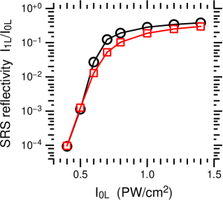
Figure 2: (Color online.) SRS reflectivity vs. pump intensity for the SRS benchmark profile of Fig. 1. The black circles and red squares are for pf3d and deplete, respectively.

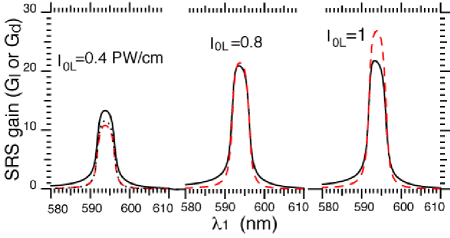
Figure 3: (Color online.) deplete gain $G_{d}$ (black solid), newlip gain $G_{l}$ (red dashed), and $G_{d}$ with no TS for $I_{0L}=0.4$ PW/cm² ($\tau_{1}=0$, black dots), for SRS benchmark. TS and volume bremsstrahlung noise enhance $G_{d}$ over $G_{l}$ for the smallest $I_{0L}$, while pump depletion suppresses $G_{d}$ for the larger two.

We also compared deplete to the massively-parallel, paraxial laser propagation code pf3d Berger et al. (1998). This code solves for the slowly-varying envelopes of the pump laser, nearly-backscattered SRS and SBS light waves, and the daughter plasma waves, in space and time. A carrier $\omega^{en}$ is chosen for each mode (except for the ion acoustic wave), and the corresponding rapid time variations are averaged over. A local eikonal $k^{en}$, given by the appropriate $\omega^{en}$ and dispersion relation with local plasma conditions, contains the rapid space variation. Kinetic quantities, such as Landau damping rates and Thomson cross-sections, are variously found from (linear) kinetic formulas or fluid approximations. There is no bremsstrahlung source, but the pump and scattered light waves all experience inverse-bremsstrahlung damping. The plasma waves undergo Landau damping, and the advection term $v_{g2}\partial_{x}n_{2}$ is retained (i.e., they are not treated in the strong damping limit). The noise source in pf3d is plasma-wave fluctuations chosen to produce the correct TS level, and uniformly distributed over a square in $k_{\perp}$ space (corresponding to the transverse $x$ and $y$ directions) extending to half the Nyquist $k$ in both $k_{x}$ and $k_{y}$.

To replicate the 1D model of deplete, we performed “plane-wave” simulations in pf3d. The incident laser at the $z=0$ entrance plane is uniform in the $x$ and $y$ directions (i.e., there is no structure like speckles), both of which are periodic with size $L_{x}=L_{y}=128\lambda_{0}$ and grid spacing $dx=dy=1.33\lambda_{0}$. The $z$ spacing is $dz=2\lambda_{0}$. As described above, the TS noise fills a square in $k_{\perp}$ space extending to $k_{x},k_{y}=\pm k_{1n}$, with $k_{1n}=(3/16)k_{0v}$ and $k_{0v}\equiv\omega_{0}/c$. We enveloped the SRS backscattered light around $\omega_{1}^{en}=0.592\omega_{0}$ ($\lambda_{1}$=593.3 nm), which has the highest linear gain. Over the slight variation of our profile, the average $k_{1}^{en}=0.461k_{0v}$.

deplete requires a solid angle $\Omega_{c}$, which we express in terms of an F-number $F$, for TS and bremsstrahlung emission (we excluded the latter for pf3d comparisons). Taking $k_{1}^{en}$ and $k_{1n}$ to determine the focal length and spot radius, one finds $F=k_{1}^{en}/2k_{1n}=1.23$. The scattered light does not uniformly fill the noise square in $k_{\perp}$ space, but rather develops into a somewhat hollow “ring” with a radius $\approx 0.12k_{0v}$ (departing more from a square for stronger pumps); there is some ambiguity in the appropriate $F$ to use. We choose $F=1$, which leads to very close reflectivities for the weakest-pump case shown in Fig. 2, and is near the noise-square estimate $F=1.23$. Sidescatter at these angles may stress the accuracy of pf3d’s paraxial approximation.

Figure 2 shows the deplete and pf3d SRS reflectivities for the benchmark profile. The pf3d values are taken at $t=$39.4 ps, after which time all reflectivities remain roughly constant (the laser ramped from zero to full strength over 10 ps). The agreement is quite good, especially in the linear (weak pump) and the strongly-depleted (strong pump) regimes. This increases confidence in the validity of the different approximations made in both codes. It took about 2 secs of wall time for deplete to run on one Itanium CPU, as opposed to 5300 secs on 16 of these CPUs for pf3d to advance 10 ps.

V.2 SBS benchmark

We performed an SBS benchmark (with SRS neglected) using the profiles in Fig. 4. The ions were fully-ionized He ($Z=2$, $A=4$) with $T_{i}=T_{e}/5$. The parallel flow velocity $u$ is shown normalized to the local acoustic speed $c_{a}^{2}\equiv(ZT_{e}+3T_{i})/Am_{p}$. The pump wavelength and profile length match the SRS benchmark. The SBS reflectivity vs. pump strength is plotted in Fig. 5, which shows pump depletion for $I_{0L}\gtrsim 1.25$ PW/cm². We estimate the absolute threshold $I_{0}^{ab}=2.6$ PW/cm² and stay below this. We used $F=1.7$ since this gives good agreement with pf3d “plane-wave” simulations for low $I_{0}$. However, for larger values of $I_{0}$ a ring in $k_{\perp}$ space develops, similar to the SRS runs, and is accompanied by a large increase in reflectivity.

Figure 6 compares the deplete and newlip gains, $G_{d}$ and $G_{l}$. For the smaller two pumps we see the enhancement of $G_{d}$ over $G_{l}$ due to TS (even though pump depletion has set in for the second case $I_{0L}=$ 1.4 PW/cm²), as discussed in Sec. VI. The dotted black curve for $I_{0L}=$ 0.6 PW/cm² is $G_{d}$ computed with no TS, and shows the modest increase in $G_{d}$ stemming from bremsstrahlung volume (as opposed to boundary) noise. The elevated plateau of $G_{d}$ to the left of the peak is also due to TS. $I_{0L}=$2.5 PW/cm² gives $G_{d}<G_{l}$ due to strong pump depletion. In all cases the wavelength and width of the main peak of the two spectra are similar. $i_{1}^{br}$, the bremsstrahlung solution, varies slightly from (4.17-4.25)$\times 10^{-9}$ W/cm²/(rad/sec) over $\lambda_{1}-\lambda_{0}=$ 20 to -3 Å.

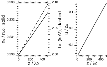
Figure 4: SBS benchmark profile.

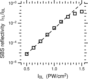
Figure 5: SBS reflectivity for SBS benchmark profile. The squares are deplete results, and the dashed line is an extension of the low-$I_{0L}$ results.

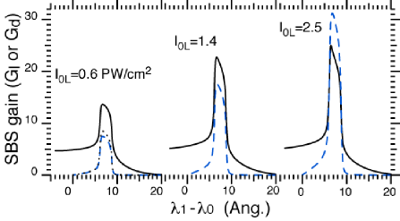
Figure 6: (Color online.) SBS deplete gain $G_{d}$ (black solid), newlip gain $G_{l}$ (blue dashed), and $G_{d}$ without TS for $I_{0L}=$0.6 PW/cm² ($\tau_{1}=0$, black dotted), for SBS benchmark profile.

VI The relation of Thomson scattering to linear gain

As seen in our benchmark runs, TS leads to an enhancement of the deplete gain compared to the newlip gain (for negligible pump depletion). This is readily seen via the scattered-wave equation with just coupling and TS, Eq. (60):

$$\partial_{z}i_{1}=-I_{0}(\tau_{1}+\Gamma_{1}i_{1}).$$ (70)

We use Eq. (51) to obtain

$$\partial_{z}i_{1}=-\gamma(i_{\tau}+i_{1}).$$ (71)

$\gamma\equiv I_{0}\Gamma_{1}$ is the spatial gain rate. Typically, $\gamma$ has a narrow peak in $z$ at the resonance point, while $i_{\tau}$ varies slowly. For simplicity, we hold $i_{\tau}$ constant at the resonance point, and solve for $i_{1}$ across the region $z=0$ to $L_{z}$ which includes the resonance. In our usual notation,

$$i_{1L}=(i_{1R}+i_{\tau})e^{G_{l}}-i_{\tau}.$$ (72)

$G_{l}\equiv\int_{0}^{L_{z}}dz\,\gamma$ is the newlip linear gain. For $G_{l}\ll 1$, $i_{1L}=i_{1R}(1+G_{l})+i_{\tau}G_{l}$, and emission due to the boundary source dominates over TS. In the opposite limit,

$$i_{1L}=(i_{1R}+i_{\tau})e^{G_{l}},\qquad e^{G_{l}}\gg 1.$$ (73)

TS therefore gives rise to an effective boundary source $i_{\tau}$ (for a narrow resonance). In this sense, it does not significantly alter the shape of the gain spectrum ($i_{\tau}$ varies slowly with $\omega_{1}$). However, it does lead to a difference in the absolute magnitude of the scattered spectrum, as embodied in an “absolutely-calibrated” gain like $G_{d}$. As an illustration, let us take $i_{1R}=i_{1}^{\mathrm{OT}}$, the optically-thick bremsstrahlung result of Eq. (39), for simplicity evaluated at the resonance point in the Jeans limit $\hbar\omega_{1}\ll T_{e}$. Moreover, we set $T_{i}=T_{e}$ so that $i_{\tau}$ assumes the simple form of Eq. (52). The effective seed is then

$$i_{1R}+i_{\tau}\rightarrow i_{1}^{\mathrm{OT}}\left(1+{\Omega_{1}\over\Omega_{1}^{v}}\psi f\eta_{0}\eta_{1}{\omega_{0}\over\omega_{1}}{\omega_{0}\over\omega_{2}^{\prime}}\right).$$ (74)

The second term on the right ($=i_{\tau}/i_{1}^{\mathrm{OT}}$) is typically $\lesssim 10$ for SRS: for our SRS benchmark, $i_{\tau}/i_{1}^{\mathrm{OT}}\approx 3$. But, it can be quite large for SBS since $\omega_{0}\gg\omega_{2}^{\prime}$ (for our SBS benchmark, $i_{\tau}/i_{1}^{\mathrm{OT}}\approx 400$). A similar result is found in Ref. Berger et al. (1989). The authors explain this on the thermodynamic ground that bremsstrahlung and Čerenkov emission (which produces TS) generate equal light- and plasma-wave action, so the light-wave energy dominates by the frequency ratio. This manifests itself in the $\omega_{0}/\omega_{2}^{\prime}$ factor in Eq. (74), which is much larger for SBS.

VII Simulation of SBS experiments

Experiments have been conducted recently at the OMEGA laser to study LPI in conditions similar to those anticipated at NIF Froula et al. (2007b). These shots use a gas-filled hohlraum, and a set of “heater” beams to pre-form the plasma environment. An “interaction” beam is propagated down the hohlraum axis after being focused through a continuous phase plate (CPP) Dixit et al. (1996) with an f/6.7 lens to a vacuum best focus of 150 $\mu$m. The plasma conditions along the interaction beam path have been measured using TS Froula et al. (2006), validating 2-dimensional hydra Marinak et al. (2001) hydrodynamic simulations that show, 700 ps after the rise of the heater beams, a uniform 1.5-mm plasma with an electron temperature of $\approx$2.7 keV Meezan et al. (2007).

Figure 7(a) displays the instantaneous SBS reflectivity increasing exponentially with the interaction beam intensity 700 ps after the rise of the heater beams. These experiments employed a 1 atmosphere gas-fill with 30% CH₄ and 70% C₃H₈ to produce an electron density along the interaction beam path of 0.06$n_{c0}$. Three-dimensional pf3d simulations agree well with the experiments Divol et al. (2008). Unlike the “plane-wave” simulations discussed in Sec. V.1, these simulations include the full speckle physics. The deplete results (blue solid curve) fall well below the experimental data in the regime where pump depletion does not play a significant role ($I_{0}\lesssim 2$ PW/cm²). This indicates that speckles are enhancing the SBS.

One way to approximate the speckle enhancement is to consider how much the coupling increases for the completely phase-conjugated mode Zel’dovich et al. (1985). This mode has a transverse intensity pattern perfectly correlated with that of the pump, over several axial ranks of speckles, and therefore enhances the coupling coefficient $\Gamma_{1}$ Divol et al. (2005). For an RPP-smoothed beam with intensity distribution $\sim e^{-I/I_{c}}$, this effectively doubles $\Gamma_{1}$. This should provide an upper bound on the reflectivity so long as the gain per speckle is $\lesssim 1$. If this is not the case, the gain in a speckled pump suffers a mathematical divergence (mitigated by pump depletion) as described in Ref. Rose and DuBois (1994). Our phase-conjugate considerations would then not apply.

The blue dashed curve in Fig. 7 shows the deplete results with twice the nominal coupling. The $2\times\Gamma_{1}$ curve is always above the experimental reflectivities. The threshold intensity for which SBS equals 5% is 1.8 PW/cm² and 0.9 PW/cm² for deplete with the nominal and twice-nominal coupling, respectively, while the experimental threshold is $\approx$1.5 PW/cm².

Comparison of deplete and pf3d is displayed in Fig. 7(b). These calculations were performed using plasma conditions from a hydra simulation, for a configuration similar to that of Fig. 7(a), but with a higher heater-beam energy. The resulting conditions are similar, except the electron temperature is higher (about 3.3 keV). The deplete reflectivity with the nominal coupling (solid blue curve) lies below the pf3d results for the two intermediate values of $I_{0}$. This demonstrates speckle effects enhance the pf3d reflectivity for moderate $I_{0}$. The deplete results for $2\times\Gamma_{1}$ (dashed blue curve) are always above the pf3d results. Preliminary analyses with deplete and pf3d of OMEGA experiments designed to study ion Landau damping in SBS Neumayer et al. (2008) also show a significant enhancement due to speckles.

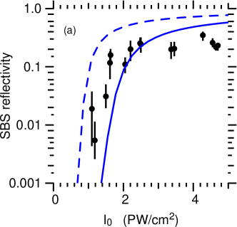
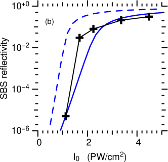
Figure 7: (Color online.) (a) SBS reflectivity for OMEGA experiments with CH gas fill and $T_{e}\approx 2.7$ keV (described in text). Black circles are measured values, the blue solid curve is deplete calculations with the nominal coupling $\Gamma_{1}$, and the blue dashed curve is deplete calculations with $2\times\Gamma_{1}$. (b) deplete and pf3d SBS reflectivities for a similar configuration but $T_{e}\approx 3.3$ keV. Black crosses are pf3d simulations, and the blue curves are the deplete results as in (a).

VIII Analysis of NIF ignition design

In this section, we exercise deplete on an actual NIF indirect-drive ignition target design. The target was designed using the hydrodynamic code lasnex Zimmerman and Kruer (1975). For more details about the design see Ref. Callahan et al. (2008); LPI analysis for this and similar ignition targets, including massively-parallel, 3D pf3d simulations, can be found in Ref. Hinkel et al. (2008). The design utilizes all 192 NIF beams (at 351 nm “blue” light), which deliver 1.3 MJ of laser energy. We analyze LPI along the 30^∘ cone of beams (one of the two “inner” cones). The pulse shape for one quad (a bundle of four beams), expressed as nominal intensity at best focus, is shown in Fig. 8, and reaches a maximum of 0.33 PW/cm². The speckle pattern for a quad approximately corresponds to an F-number of $F=8$, which we use for deplete’s noise sources (but each beam individually has $F=20$ optics). The focal spot is elliptical with semi-axis lengths of 693, 968 $\mathrm{\mu m}$. The peak temperature of the radiation drive is 285 eV. The materials are as follows: the capsule ablator is Be, a plastic (CH) liner surrounds the laser entrance hole, the hohlraum wall is Au-U with a thin outer layer of 80% Au-20% B (atomic ratio), and the initial fill gas is 80% H-20% He. The lower-Z components are included in the last two mixtures to reduce SBS by increasing the ion Landau damping of the acoustic wave.

Figure 8: Nominal intensity at best focus for 285 eV NIF ignition design (“NIF example”), found by dividing the laser power per quad by the focal spot size. The peak intensity corresponds to 6.9 TW/quad.

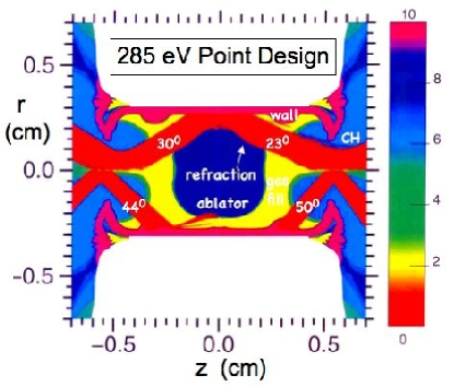
Figure 9: (Color online.) Materials and laser beam cones for NIF example.

We performed deplete calculations, with both SRS and SBS, at several times and over 381 ray paths for each time. One must take an appropriate “average” over the rays to characterize the LPI on a cone. Regarding newlip gains, this has led to several approaches. These include averaging the gain, finding the maximum gain, or averaging $e^{G_{l}}$. This last method stems from assuming there is no pump depletion and noise sources are independent of scattered frequency; in this limit, the reflectivity should be roughly proportional to $e^{G_{l}}$. However, this averaging, and a fortiori taking the maximum, can be dominated by gains that are larger than physically allowed by pump depletion or other nonlinearity. One can attempt to include pump depletion via a Tang formula for $G_{l}$ at each $\omega_{1}$ Tang (1966).

deplete allows for more physical ray-averaging schemes. To the extent the transverse intensity pattern of a cone is uniform, each ray represents the same incident laser power. Averaging deplete’s ray reflectivities then measures the fraction of incident power that gets reflected. Pump depletion is of course included, which limits backscatter along high-gain rays in a physical way. The reflectivities and scattered spectra plotted here are simple averages over the rays.

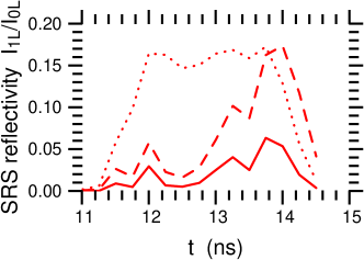
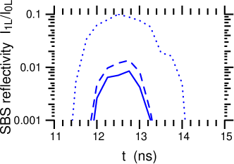
Figure 10: (Color online.) deplete SRS and SBS ray-averaged reflectivities $I_{1L}$ for NIF example. Solid lines are the nominal case (re-absorption and $\Gamma_{1}$ unscaled), dashed lines are the nominal $\Gamma_{1}$ but no re-absorption of scattered light ($\kappa_{1}=0$), and dotted lines are $2\times\Gamma_{1}$ with re-absorption.

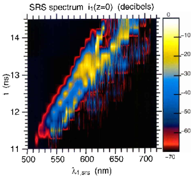
Figure 11: (Color online.) SRS streaked spectrum $i_{1L}$ for NIF example, nominal case ($\kappa_{1}\neq 0$, $1\times\Gamma_{1}$).

Figure 12: (Color online.) SBS streaked spectrum for NIF example, nominal case ($\kappa_{1}\neq 0$, $1\times\Gamma_{1}$). The white-yellow streak from 5-8 Å occurs in the Be ablator, while the weaker feature from 12-15 Å occurs in the gas fill.

The reflectivities for several times near peak laser power, for the 30^∘ cone, are shown in Fig. 10. The results for three different cases are presented. First, the solid lines give the reflectivities computed with the unmodified deplete equations. To quantify the role of re-absorption of scattered light in the target, we re-ran deplete with $\kappa_{1}=0$. This leads to the dashed lines. Finally, to bound the enhancement due to speckles, we plot the results when $\Gamma_{1}$ is doubled (and $\kappa_{1}\neq 0$) as the dotted lines.

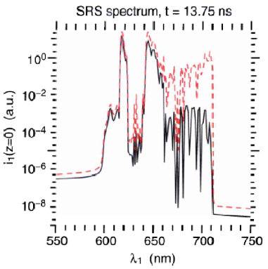
Figure 13: (Color online.) deplete SRS spectrum at time 13.75 ns for NIF example, smoothed over $\approx 1$ nm. The black solid and red dashed lines are computed with ($\kappa_{1}\neq 0$) and without ($\kappa_{1}=0$) re-absorption of scattered light, respectively.

The spectra of escaping SRS and SBS light (averaged over rays) are shown in Fig. 11-12. The SBS feature at a wavelength shift of 5-8 Å comes from the Be ablator blowoff. A much weaker feature appears from 12-13 ns at 12-15 Å, and occurs in the gas fill. The SRS spectrum is more irregular, showing two main features separated by $\approx$20 nm that move to higher $\lambda_{1}$ as time increases. In addition, there are narrow features at higher $\lambda_{1}$ that originate near the hohlraum wall; these would be reduced in a ray-averaged gain, since the exact $\lambda_{1}$ active for each ray depends sensitively on conditions near the wall and therefore varies from ray to ray. Re-absorption strongly suppresses these high-$\lambda_{1}$ spikes, as is seen in the SRS spectra with and without re-absorption at $t=$ 13.75 ns in Fig. 13. Collisional plasma-wave damping, currently not in deplete, may reduce the high-$\lambda_{1}$ scattering (the Landau damping of the low-$k_{2}\lambda_{De}$ plasma waves is negligible).

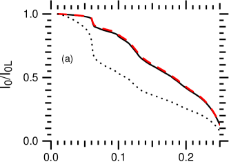
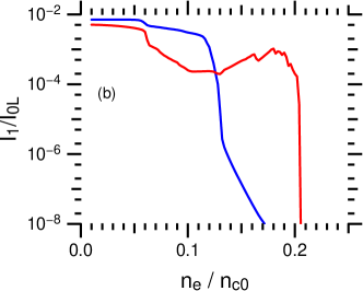
Figure 14: (Color online.) (a) Laser transmission for NIF example at 12.5 ns (peak power): black solid curve is the nominal deplete solution with pump depletion, red dashed curve is with just inverse-bremsstrahlung absorption, and black dotted curve is the deplete solution with $2\times\Gamma_{1}$. (b) SBS (blue) and SRS (red) scattered intensities for the nominal deplete solution. Calculation of intensity at a given $n_{e}$ is described in text.

Besides backscatter, deplete also provides the pump intensity $I_{0}(z)$ along each ray. This indicates how much laser energy is transmitted to a given location, which is a crucial aspect of a whether LPI degrades target performance. In cases where the backscattered light undergoes significant absorption as it propagates out of the target (as happens to SRS for the design analyzed here), the measured reflectivity can understate the level of LPI. The laser transmission can reveal this fact. Figure 14(a) presents $I_{0}$, averaged over all the rays, at a given $n_{e}$. This is a 1D presentation of how much energy reaches a given density, although in the full 3D geometry different rays reach the same $n_{e}$ at different locations. $I_{0}$ with just pump absorption, as well as the deplete solutions with pump depletion for the nominal case and $2\times\Gamma_{1}$, are shown. Pump depletion is barely discernible in the nominal case, but is significant in the $2\times\Gamma_{1}$ case. For instance, in the latter case $I_{0}$ at $n_{e}/n_{c0}=0.2$ is only 60% of its absorption-only value. The wavelength-integrated SRS and SBS $I_{1}$ are shown in Fig. 14(b), and the scattered spectra vs. $n_{e}$ are shown in Figs. 15-16. SRS in particular develops at several different densities, corresponding to different wavelengths, as can be seen in Figs. 13 and 15.

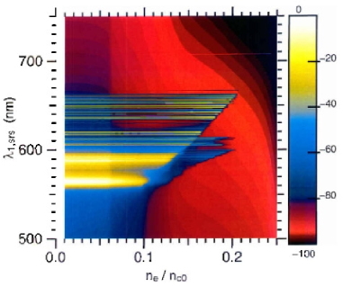
Figure 15: (Color online.) SRS spectral density $i_{1}$ vs. $n_{e}/n_{c0}$ and $\lambda_{1}$, in decibels, at 12.5 ns (peak power), for NIF example.

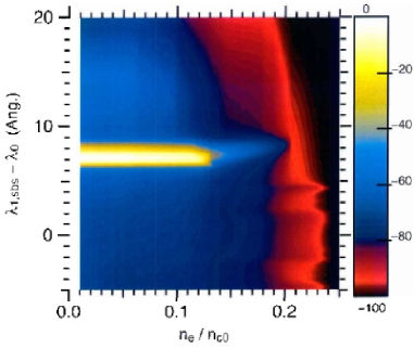
Figure 16: (Color online.) SBS spectral density $i_{1}$ vs. $n_{e}/n_{c0}$ and $\lambda_{1}-\lambda_{0}$, in decibels, at 12.5 ns (peak power), for NIF example.

IX Conclusions and future prospects

We have derived a 1D, steady-state, kinetic model for Brillouin and Raman backscatter, that includes pump depletion, bremsstrahlung damping and fluctuations, and Thomson scattering. This model is implemented by the code deplete, which we have presented as well. This work extends linear gain calculations, by including more physics while retaining its low computational cost. In particular, deplete provides the scattered-light spectrum and intensity developing from physical noise, which can be compared against more sophisticated codes and experiments. The transmitted pump laser along the profile is also found, which is important for assessing an ICF target design, especially when re-absorption of scattered light reduces the escaping backscatter from its internal level.

We presented benchmarks of deplete on contrived, linear profiles, as well as analysis of OMEGA experiments and a NIF ignition design. The benchmarks reveal the deficiencies of linear gain, namely the neglect of TS, pump depletion, and re-absorption. Comparisons with pf3d provide a cross-validation of the two codes in a regime where they should agree. The OMEGA SBS experimental data, as well as pf3d simulations of these shots, show much more reflectivity than deplete gives, for intensities where pump depletion is weak. This enhancement is due to speckle effects. We showed an upper bound on this enhancement is given by doubling the deplete coupling coefficient $\Gamma_{1}$, which comes from considering the phase-conjugated mode in an RPP-smoothed beam. The ignition design analysis gives reasonably low backscatter levels for the nominal laser intensity and including re-absorption, with SRS dominating SBS. However, if re-absorption is neglected, or especially if $\Gamma_{1}$ is doubled, the backscatter appears more worrisome. The laser transmission supports these conclusions.

Ray-based gain calculations have been used for some time to model LPI experiments, and deplete can provide more detailed comparisons. An early application of gain to hohlraum targets is Ref. Glenzer et al. (2001), where hohlraums filled with CH gas were driven by laser beams with and without PS and SSD. Without SSD, reasonable agreement was found between measurments and the time-dependent SBS gain spectrum. However, there was a large difference in peak SRS wavelength between measurements and the gain spectrum, which may be due to laser filamentation changing the location of peak SRS growth.

Several future directions exist for deplete. One is to include an “independent speckle” model for gain enhancement, where one solves the deplete equations over a speckle length for a distribution of pump intensities and then re-distributes the power. This would not describe correlations among axial ranks of speckles, caused e.g. by phase conjugation. deplete also enables some new diagnostics and applications. The pump and scattered intensities found by deplete can be used to compute the local material heating rate due to absorption. This could be incorporated into a hydrodynamic code, thereby coupling LPI to target evolution in a self-consistent, if simplified, way. In addition, the plasma-wave amplitudes found by deplete can be compared against thresholds for various nonlinearities to assess their relevance, and may allow estimation of hot electron production by SRS.

Despite its promise, there are limits inherent to any 1D or ray-based approach, stemming from 3D wave optics (e.g. diffraction, speckles, filamentation, and beam bending). A 3D paraxial code called slip Froula et al. (2008), which like deplete operates in steady state and uses kinetic coefficients, is being developed. This model is in some sense intermediate between deplete and pf3d. 1D codes like deplete still have a valuable role. They can analyze hundreds of rays, using hundreds of scattered wavelengths, in $\sim$ minutes, thus allowing designs to be rapidly analyzed and compared. The resulting time-dependent spectra allow for contact with experimental diagnostics, and are frequently needed, for example, to choose the carrier $k$ and $\omega$ for pf3d.

Laser-plasma interactions have proven to be a very challenging area of plasma physics, owing to the variety of relevant physics and extreme range of scales involved. This has led to an equally extreme range of modeling tools, from 1D gain estimates to 3D kinetic simulations. By fully exploiting these tools, each with their uses and limitations, a more complete picture is emerging.

Appendix A newlip

In this appendix, we document the laser interaction post-processor newlip, of which deplete can be viewed as an extension. The equations underlying newlip are

$$d_{z}I_{0}(z) = -\kappa_{0}I_{0},$$ (75)

$$\partial_{z}i_{1}(z,\omega_{1}) = -I_{0}\Gamma_{1}i_{1}.$$ (76)

The first of these is Eq. (54) with no pump depletion ($\tau_{1}=\Gamma_{1}=0$), and the second is Eq. (55) with no bremsstrahlung or TS ($\kappa_{1}=\Sigma_{1}=\tau_{1}=0$). That is, only the absorption of the pump, and coherent coupling to scattered light waves, are modeled. The boundary conditions are $I_{0}(z=0)=I_{0L}$ (the known pump at the laser entrance), and $i_{1}(z=L_{z},\omega_{1})=1$. We thus solve for a unit scattered-wave boundary seed, which is permissible for this linear system.

We readily solve Eqs. (75-76) to find

$$I_{0}(z) = I_{0L}e^{-\int_{0}^{z}dz^{\prime}\ \kappa_{0}(z^{\prime})},$$ (77)

$$i_{1}(z) = e^{G_{l}(z)},$$ (78)

$$G_{l}(z) \equiv \int_{z}^{L_{z}}dz^{\prime}\ \Gamma_{1}(z^{\prime})I_{0}(z^{\prime}).$$ (79)

$G_{l}(z)$ is the linear intensity gain exponent, and is newlip’s main result. The total gain across the profile is $G_{l}(z=0)$.

The numerical computation of $G_{l}$ suffers from the problem of narrow resonances, similar to deplete. The coupling coefficient $\Gamma_{1}$ (see Eq. (17)) is sharply peaked near the resonance point where $\mathrm{Re}\,\epsilon=0$. newlip addresses this challenge in a way analogous to how deplete handles the coupling-Thomson step, as outlined in Appendix B. In particular, the integration of Eq. (76) from $z^{n}$ down to $z^{n-1}$ can be cast in the form

$$\ln{i_{1}^{n-1}\over i_{1}^{n}}=\mathrm{Im}\,S_{0},\qquad S_{0}\equiv\int_{z^{n}}^{z^{n-1}}dz\ {S\over\epsilon},$$ (80)

with $S\equiv-I_{0}f\Gamma_{S}\chi_{e}(1+\chi_{I})$. Although $S(z)/\epsilon(z)$ is sharply-peaked near resonance, $S(z)$ and $\epsilon(z)$ are themselves slowly-varying with $z$. We approximate $S(z)\approx S^{n-1/2}+(z-z^{n-1/2})\Delta S/\Delta z$ (and similarly for $\epsilon$), with $X^{n-1/2}\equiv(X^{n}+X^{n-1})/2$ and $\Delta X\equiv(X^{n}-X^{n-1})$ for some quantity $X$ . With this representation, and $\hat{X}\equiv X^{n-1/2}/\Delta X$, we find

$$S_{0}={\Delta z\Delta S\over\Delta\epsilon}\left[1+(\hat{\epsilon}-\hat{S})\ln{\epsilon^{n-1}\over\epsilon^{n}}\right].$$ (81)

This formula is valid provided either $|\mathrm{Re}\,\hat{\epsilon}|\geq 1/2$ or $\mathrm{Im}\,\hat{\epsilon}\neq 0$. For accuracy, we also want $|\Delta\epsilon|$ to not be too small (which obtains, e.g., for a flat profile). We therefore require $|\hat{\epsilon}|$ to be less than some large number. If any of these conditions does not hold, we simply assume $S=S^{n-1/2}$ and $\epsilon=\epsilon^{n-1/2}$ across the cell to find

$$S_{0}=\Delta z{S^{n-1/2}\over\epsilon^{n-1/2}}.$$ (82)

Appendix B Numerical solution of the coupling-Thomson step

This appendix provides a derivation of Eq. (67), the solution for $i_{1}$ in the coupling-Thomson step. We must solve Eq. (60), from $z^{n}$ down to $z^{n-1}$, with $I_{0}=I_{0}^{n}$ and all coefficients except $|\epsilon|^{2}$ evaluated at $z^{n-1/2}$. We write this equation as

$$\partial_{z}i_{1} = -{K_{\tau}+K_{\Gamma}i_{1}\over|\epsilon|^{2}},$$ (83)

$$K_{\tau} \equiv I_{0}^{n}\tau_{S}^{n-1/2}g_{\tau}^{n-1/2},\quad K_{\Gamma}\equiv fI_{0}^{n}\Gamma_{S}^{n-1/2}g_{\Gamma}^{n-1/2}.$$ (84)

As mentioned above, the principal numerical difficulty is that $|\epsilon|^{-2}$ is sharply peaked near resonance ($\mathrm{Re}\,\epsilon=0$). Since $\mathrm{Re}\,\epsilon$ generally passes through zero slowly, we Taylor expand $\epsilon$ within each zone and solve the resulting system analytically.

Define the zonal average and difference $X^{n-1/2}\equiv(1/2)(X^{n}+X^{n-1})$ and $\Delta X\equiv X^{n}-X^{n-1}$ for the quantity $X$. We expand $\epsilon$ about the zone center $z^{n-1/2}$ to find

$$\epsilon \approx \epsilon^{n-1/2}+\hat{z}\Delta\epsilon,$$ (85)

$$\hat{z} \equiv {z-z^{n-1/2}\over\Delta z}.$$ (86)

We can then write

$$|\epsilon|^{2} = \epsilon_{1}+|\Delta\epsilon|^{2}(\hat{z}-\hat{z}_{0})^{2},$$ (87)

$$\epsilon_{1} \equiv |\Delta\epsilon|^{-2}\mathrm{Im}\left[\epsilon^{n-1/2}\Delta\epsilon^{*}\right]^{2},$$ (88)

$$\hat{z}_{0} \equiv -|\Delta\epsilon|^{-2}\mathrm{Re}\left[\epsilon^{n-1/2}\Delta\epsilon^{*}\right].$$ (89)

The linear change of variable

$$s\equiv{|\Delta\epsilon|\over\sqrt{\epsilon_{1}}}(\hat{z}-\hat{z}_{0})$$ (90)

transforms Eq. (83) to

$$\partial_{s}i_{1} = -{B_{\tau}+B_{\Gamma}i_{1}\over 1+s^{2}},$$ (91)

$$B_{\tau,\Gamma} \equiv {K_{\tau,\Gamma}\Delta z\over|\mathrm{Im}\left[\epsilon^{n-1/2}\Delta\epsilon^{*}\right]|}.$$ (92)

A second change of variable to $w\equiv\mathrm{atan}\ s$ yields

$$\partial_{w}i_{1}=-(B_{\tau}+B_{\Gamma}i_{1}).$$ (93)

This equation is solved to give the result used in Eq. (67):

$$i_{1}^{n-1} = (i_{1}^{n}+i_{\tau})e^{B_{\Gamma}\Delta w_{n}}-i_{\tau},$$ (94)

$$\Delta w_{n} \equiv \mathrm{atan}\ s^{n}-\mathrm{atan}\ s^{n-1}.$$ (95)

$i_{\tau}=B_{\tau}/B_{\Gamma}$ is also given by Eq. (51).

If $\Delta\epsilon$ is sufficiently small (or zero, as for a flat profile), we do not use Eq. (85), but instead $\epsilon\approx\epsilon^{n-1/2}$. We can then immediately solve Eq. (83) to find

$$i_{1}^{n-1}=(i_{1}^{n}+i_{\tau})\exp\left[{K_{\Gamma}|\epsilon^{n-1/2}|^{-2}\Delta z}\right]-i_{\tau}.$$ (96)

References

- Kruer (2003) W. L. Kruer, The Physics of Laser Plasma Interactions (Westview Press, Boulder, CO, 2003).
- Tajima and Dawson (1979) T. Tajima and J. M. Dawson, Phys. Rev. Lett. 43, 267 (1979).
- Malkin et al. (1999) V. M. Malkin, G. Shvets, and N. J. Fisch, Phys. Rev. Lett. 82, 4448 (1999).
- Atzeni and ter Vehn (2004) S. Atzeni and J. M. ter Vehn, The Physics of Inertial Fusion: Beam Plasma Interaction, Hydrodynamics, Hot Dense Matter (Oxford University Press, Oxford, UK, 2004).
- Lindl et al. (2004) J. Lindl, P. Amendt, R. L. Berger, S. G. Glendinning, S. H. Glenzer, S. W. Haan, R. L. Kauffman, O. L. Landen, and L. J. Suter, Phys. Plasmas 11, 339 (2004).
- Berger et al. (1989) R. L. Berger, E. A. Williams, and A. Simon, Phys. Fluids B 1, 414 (1989).
- Ramani and Max (1983) A. Ramani and C. E. Max, Phys. Fluids 26, 1079 (1983).
- Mounaix et al. (1997) P. Mounaix, D. Pesme, and M. Casanova, Phys. Rev. E 55, 4653 (1997).
- Froula et al. (2007a) D. H. Froula, L. Divol, N. B. Meezan, S. Dixit, J. D. Moody, P. Neumayer, B. B. Pollock, J. S. Ross, and S. H. Glenzer, Phys. Rev. Lett. 98, 085001 (2007a).
- Neumayer et al. (2008) P. Neumayer, R. L. Berger, L. Divol, D. H. Froula, R. A. London, B. J. MacGowan, N. B. Meezan, J. S. Ross, C. Sorce, L. J. Suter, and S. H. Glenzer, Phys. Rev. Lett. 100, 105001 (2008).
- Boehly et al. (1997) T. R. Boehly, D. L. Brown, R. S. Craxton, R. L. Keck, J. P. Knauer, J. H. Kelly, T. J. Kessler, S. A. Kumpan, S. J. Loucks, S. A. Letzring, F. J. Marhsall, R. L. McCrory, S. F. B. Morse, W. Seka, J. M. Soures, and C. P. Verdon, Opt. Commun. 133, 495 (1997).
- Paisner et al. (1994) J. A. Paisner, E. M. Campbell, and W. J. Hogan, Fusion Technol. 26, 755 (1994).
- Dewandre et al. (1981) T. Dewandre, J. R. Albritton, and E. A. Williams, Phys. Fluids 24, 528 (1981).
- Bers (1975) A. Bers, in Physique des Plasmas - Les Houches 1972, edited by C. DeWitt and J. Peyraud (Gordon and Breach, New York, 1975).
- Cohen and Kaufman (1977) B. I. Cohen and A. N. Kaufman, Phys. Fluids 20, 1113 (1977).
- Fried and Conte (1961) B. D. Fried and S. D. Conte, The Plasma Dispersion Function: The Hilbert Transform of the Gaussian (Academic Press, New York, 1961).
- Abramowitz and Stegun (1970) M. Abramowitz and I. A. Stegun, Handbook of Mathematical Functions (Dover Publications, Inc., New York, NY, 1970).
- Bekefi (1966) G. Bekefi, Radiation Processes in Plasmas (John Wiley and Sons, New York, 1966).
- Dawson and Oberman (1962) J. Dawson and C. Oberman, Phys. Fluids 5, 517 (1962).
- Oberman and Williams (1983) C. R. Oberman and E. A. Williams, in Handbook of Plasma Physics, Vol. 1, edited by M. N. Rosenbluth and R. Z. Sagdeev (North-Holland, Amsterdam, 1983), chap. 2.3.
- Evans (1970) D. E. Evans, Plasma Phys. 12, 573 (1970).
- Milonni and Eberly (1988) P. W. Milonni and J. H. Eberly, Lasers (John Wiley & Sons, 1988).
- Hinkel et al. (1999) D. E. Hinkel, R. L. Berger, E. A. Williams, A. B. Langdon, C. H. Still, and B. F. Lasinski, Phys. Plasmas 6, 571 (1999).
- Froula et al. (2008) D. H. Froula, L. Divol, R. A. London, P. Michel, R. L. Berger, N. B. Meezan, P. Neumayer, J. S. Ross, R. Wallace, and S. H. Glenzer, Phys. Rev. Lett. 100, 015002 (2008).
- Strang (1968) G. Strang, SIAM J. Numer. Anal. 5, 506 (1968).
- Yanencko (1970) N. N. Yanencko, The Method of Fractional Steps (Springer-Verlag, New York, 1970).
- Tang (1966) C. L. Tang, J. Appl. Phys. 37, 2945 (1966).
- Berger et al. (1998) R. L. Berger, C. H. Still, E. A. Williams, and A. B. Langdon, Phys. Plasmas 5, 4337 (1998).
- Froula et al. (2007b) D. H. Froula, L. Divol, N. B. Meezan, S. Dixit, P. Neumayer, J. D. Moody, B. B. Pollock, J. S. Ross, L. Suter, and S. H. Glenzer, Phys. Plasmas 14, 055705 (2007b).
- Dixit et al. (1996) S. N. Dixit, M. D. Feit, M. D. Perry, and H. T. Powell, Opt. Lett. 21, 1715 (1996).
- Froula et al. (2006) D. H. Froula, J. S. Ross, L. Divol, N. Meezan, A. J. MacKinnon, R. Wallace, and S. H. Glenzer, Phys. Plasmas 13, 052704 (2006).
- Marinak et al. (2001) M. M. Marinak, G. D. Kerbel, N. A. Gentile, O. Jones, D. Munro, S. Pollaine, T. R. Dittrich, and S. W. Haan, Phys. Plasmas 8, 2275 (2001).
- Meezan et al. (2007) N. B. Meezan, R. L. Berger, L. Divol, D. H. Froula, D. E. Hinkel, O. S. Jones, R. A. London, J. D. Moody, M. M. Marinak, C. Niemann, P. B. Neumayer, S. T. Prisbrey, J. S. Ross, E. A. Williams, S. H. Glenzer, and L. J. Suter, Phys. Plasmas 14, 056304 (2007).
- Divol et al. (2008) L. Divol, R. L. Berger, N. B. Meezan, D. H. Froula, S. Dixit, P. Michel, R. London, D. Strozzi, J. Ross, E. A. Williams, B. Still, L. J. Suter, and S. H. Glenzer, Phys. Plasmas 15, 056313 (2008).
- Zel’dovich et al. (1985) B. Y. Zel’dovich, N. F. Pilipetsky, and V. V. Shkunov, Principles of Phase Conjugation (Springer-Verlag, Berlin, 1985).
- Divol et al. (2005) L. Divol, E. A. Wiliams, R. L. Berger, and D. E. Hinkel, Bull. Am. Phys. Soc. 50 (2005).
- Rose and DuBois (1994) H. A. Rose and D. F. DuBois, Phys. Rev. Lett. 72, 2883 (1994).
- Zimmerman and Kruer (1975) G. Zimmerman and W. L. Kruer, Comments Plasma Phys. Controlled Fusion 2, 85 (1975).
- Callahan et al. (2008) D. A. Callahan, D. E. Hinkel, R. L. Berger, L. Divol, S. N. Dixit, M. J. Edwards, S. W. Haan, O. S. Jones, J. D. Lindl, N. B. Meezan, P. A. Michel, S. M. Pollaine, L. J. Suter, R. P. J. Town, and P. A. Bradley, IFSA 2007 proceedings, Journ. Physics: Conference Series (2008).
- Hinkel et al. (2008) D. E. Hinkel, D. A. Callahan, A. B. Langdon, S. H. Langer, C. H. Still, and E. A. Williams, Phys. Plasmas 15, 056314 (2008).
- Glenzer et al. (2001) S. H. Glenzer, R. L. Berger, L. M. Divol, R. K. Kirkwood, B. J. MacGowan, J. D. Moody, A. B. Langdon, L. J. Suter, and E. A. Williams, Phys. Plasmas 8, 1692 (2001).