A Low-Mass Planet with a Possible Sub-Stellar-Mass Host in Microlensing Event MOA-2007-BLG-192
Abstract
We report the detection of an extrasolar planet of mass ratio in microlensing event MOA-2007-BLG-192. The best fit microlensing model shows both the microlensing parallax and finite source effects, and these can be combined to obtain the lens masses of for the primary and for the planet. However, the observational coverage of the planetary deviation is sparse and incomplete, and the radius of the source was estimated without the benefit of a source star color measurement. As a result, the 2- limits on the mass ratio and finite source measurements are weak. Nevertheless, the microlensing parallax signal clearly favors a sub-stellar mass planetary host, and the measurement of finite source effects in the light curve supports this conclusion. Adaptive optics images taken with the Very Large Telescope (VLT) NACO instrument are consistent with a lens star that is either a brown dwarf or a star at the bottom of the main sequence. Follow-up VLT and/or Hubble Space Telescope (HST) observations will either confirm that the primary is a brown dwarf or detect the low-mass lens star and enable a precise determination of its mass. In either case, the lens star, MOA-2007-BLG-192L, is the lowest mass primary known to have a companion with a planetary mass ratio, and the planet, MOA-2007-BLG-192Lb, is probably the lowest mass exoplanet found to date, aside from the lowest mass pulsar planet.
1 Introduction
When the first extrasolar planets were discovered orbiting main sequence stars more than a decade ago (Mayor & Queloz, 1995; Marcy & Butler, 1996; Butler & Marcy, 1996), the radial velocity surveys responsible for the discoveries focused their observations on stars of spectral type F, G, and K, because such stars offered the greatest planet detection sensitivity. However, observations of star forming regions indicate that stars of virtually all types have evidence of proto-planetary disks, suggesting that the first stages of the planet formation are practically independent of star type. The radial velocity surveys have since expanded their target lists to include stars ranging from a spectral type of mid-M to stars that are thought to have spectral type A when they were on the main sequence. Gas giant planets have been found in orbit around stars of all these types (Butler et al., 2006; Sato et al., 2007; Johnson et al., 2007; Niedzielski et al., 2007; Lovis & Mayor, 2007), but they appear to be increasingly rare in orbit around low-mass stars.
In the past few years, microlensing surveys (Bennett, 2008) have extended the range of sensitivity to cool, “super-Earth” planets (Beaulieu et al., 2006; Gould et al., 2006) with masses of in orbits beyond the “snow-line” (Ida & Lin, 2004; Laughlin, Bodenheimer & Adams, 2004; Kennedy et al., 2006), where the core accretion theory predicts that the most massive planets should form. These discoveries indicate that such low-mass planets are significantly more common than gas giants in orbit around the stars of that are probed by the microlensing method. Because microlensing does not rely upon light from the planetary host star in order to detect the planet, its sensitivity extends to host star masses well below the lower limit for current radial velocity surveys.
In this paper, we present the analysis of microlensing event MOA-2007-BLG-192, and show that the lens system is likely to be a low-mass planet orbiting a primary that is either a brown dwarf or a very low-mass main sequence star. The data are discussed in § 2, and the planetary nature of the light curve is discussed in § 3. The uncertainties in the microlensing model parameters are discussed in § 4, and in § 5, we show that the microlensing parallax and finite source features of the light curve favor a sub-stellar mass primary and a very low-mass planet. Adaptive optics images from the VLT NACO instrument are only consistent with a primary lens mass that is a brown dwarf or a star at the bottom of the main sequence. In § 6, we show how future observations with VLT/NACO can confirm this interpretation and determine the parameters of the planetary system more precisely.
2 Data
The discovery of microlensing event MOA-2007-BLG-192 was triggered by data from the night of peak magnification, 2007 May 24 UT, when planetary deviation occurred. The faintness of the source star and poor weather at the MOA telescope during the night prior to peak magnification prevented earlier detection of this event by MOA.
The 2.2 square degree field of the MOA-cam3, mounted on the the 1.8m MOA-II telescope (Sako et al., 2007; Hearnshaw et al., 2005) allows 50 square degrees of the Galactic bulge to be observed every hour, and it was this frequent sampling of this event that resulted in the detection of the planetary signal, despite the lack of an early alert. Continuing improvements in the MOA photometry and alert system (Bond et al., 2001) should allow a similar event to be alerted earlier in future seasons.
The photometry of the MOA data was performed with a custom version of the MOA pipeline that is optimized for precise photometry of selected events. When an event is detected, a collection of small pixel “cameo” images is generated from all the images taken that season. These small images provide more precise coordinate transformations and cleaner subtracted images, resulting in more precise photometry. We selected the best MOA photometry from multiple runs with different photometry code parameters by comparing light curve fits to the data outside of the planetary deviation. The photometry of the light curve peak, which is critical for the planetary interpretation was confirmed by multiple photometry codes including the OGLE pipeline (Udalski, 2003a). The MOA data set consists of 718 observations from the 2007 season.
This event was not among the events per year found by the OGLE Early Warning System (Udalski et al., 1994) because the source star was too faint to appear in the OGLE star catalog used for online photometry. However, a star catalog based upon a recent OGLE image with 0.75” seeing does include the MOA-2007-BLG-192 source star. The OGLE photometry was obtained with the standard OGLE photometry pipeline with this good seeing reference image, and the resulting data set consists of 442 observations dating back to 2001.
In the crowded stellar fields where microlensing events are observed, the true photometric errors often depend on the proximity of nearby stars. As a result, it is customary to rescale the error bars to give for each telescope/passband. For this event, these scaling factors were determined with a single lens fit excluding the data taken in a 24-hour period centered on the planetary light curve deviation. We find that no rescaling is needed for the MOA data, while the OGLE error bars are slightly overestimated. Both data sets have a 0.1% systematic uncertainty added in quadrature, and the reported OGLE error bars are reduced by a factor of 0.92.
3 Planetary Nature of the Light Curve
This event is an example of a high magnification event, which allows the detection of planets via perturbations of the central or “stellar” caustic (Griest & Safizadeh, 1998; Rhie et al., 2000; Rattenbury et al, 2002; Udalski et al., 2005; Gould et al., 2006; Gaudi et al., 2008). But close or wide stellar binary lens systems can also give light curve perturbations at high magnification (Albrow et al., 2002; Abe et al., 2003), so it is important to distinguish between these two possibilities. Also, the incomplete coverage of the light curve may allow multiple binary lens models, so it is important to do a careful search of parameter space to ensure that all viable models are found.
We have carefully searched parameter space to find the best fit planetary and stellar binary lens models, and these best fit models are displayed in Figure 1 with the solid black curve indicating the best fit planetary model and the green curve in the right hand panel indicating the best fit stellar binary model. Figure 1 shows the magnified portion of the MOA-2007-BLG-192 light curve, with a close-up of the light curve peak shown in the lower panel. These plots are made in linear flux units normalized to the flux of the best fit planetary lens model, which has a source magnitude of . The black and blue curves indicate the best fit model as seen from the MOA and OGLE telescopes, respectively. These light curves are slightly different due to the different microlensing magnification observed from the sites of the different telescopes. This effect is known as terrestrial parallax and was first discussed by Holz & Wald (1996). For all the other models, only the light curve as seen by MOA is shown.
The grey curve is a caustic crossing planetary model, which has a similar and planetary parameters to the best fit planetary model, but has a very different caustic structure. In fact, the fit is slightly lower than the “best” model, but this slight improvement is more than offset by the lower a priori probability of the parameters. The short-dashed cyan and magenta curves represent the 2- lower and upper limits on the planetary mass ratio, , so they have a value that is larger than the best model by . The reasons why these models provide the lower and upper mass ratio limits are clear from the light curve plot. The lower mass ratio limit light curve (cyan) puts the last MOA observation on the planetary deviation at the minimum between the two cusp approach peaks. At smaller , the separation between these cusps would grow smaller, which would tend to increase the brightness at the time of this observation (). The upper limit model (magenta) has a much larger cusp approach separation and has pushed the second cusp approach to where it begins to affect the OGLE observation at . Thus, the planetary models are constrained to have the second cusp approach appear in the time interval where it is not constrained by the data. Similar arguments can be made with regard to the caustic crossing model shown by the grey curve, but the limits on for the caustic crossing models are tighter than the limits on the cusp approach models.
The long-dashed green curve is the best fit stellar binary model, which is able to reproduce the observed light curve to within a few percent. But, it does not provide a good fit to the data. The best fit model has for 1160 data points and 13 model parameters to give , while the best fit stellar binary model gives , a difference of .
The reason why the stellar binary models fail can be understood based upon the basic properties of the central caustics of stellar binary light curves, i.e. those without an extreme mass ratio. The central caustics of such binaries are quite strong, so they provide very strong light curve deviations that extend far from the light curve peak unless they are kept very small by making the binary separation, , very much smaller or very much larger than the Einstein ring radius. This forces the caustics to the diamond shaped form shown in Figure 3(f).
Figure 2 shows the parameter space locations of the models that can provide an approximate fit to the light curve data with a value within 360 of the best fit as a function of the mass ratio, , and the angle between the lens axis and the direction of the lens-source relative motion, . For stellar binary solutions, with , this figure indicates an approximate 4-fold degeneracy, with the best solutions at each value separated by .
The situation is different for the planetary models with . Figure 2 shows that only two of these solutions continue to give moderately low values in the planetary regime. So, the approximate symmetry at large has morphed into an approximate symmetry at small . This is easily understood as following from the basic properties of the central caustics of binary lens light curves (Dominik, 1999). The central caustic for the best fit stellar binary model is shown in Figure 3(f). This model has a mass ratio of , but the central caustic has a nearly perfect rotation symmetry. The regions of higher magnification extend outward from the cusps of these caustic curves, and so one of the cusps points at the location of the source at in order to account of the observed bump in the light curve. But, the symmetry enforces a minimum day delay between the observed cusp approach and the next one. This ensures that the 2nd cusp approach will have some effect on the OGLE data point at .
Figures 3(a), (b), and (c) show the caustic curves and source trajectories for the best fit and the 2- lower and upper limit (on ) models. The red and blue circles indicate the location and relative size of the source star at the time of the MOA and OGLE images, respectively. The magnification deviations due to these central caustics extend outward from the cusps, but the cusps in these planetary models always point in a direction quite close to the lens axis. Thus, the two sets of planetary solutions shown in Figure 2 correspond to the cases where the source crosses the single “forward” cusp or approaches the multiple cusps pointing “backwards.” (There are always three cusps pointing “backwards” as shown in Figure 3(c), but when the planet is close to the Einstein ring, as is the case for the small solutions, the central caustic on the “back” side becomes so weak as to be invisible in these figures.)
The caustic geometries of two caustic crossing models are shown in Figures 3(d) and (e). The model given by the grey curve in Figure 1 corresponds to Figure 3(d), while the light curve corresponding to Figure 3(e) is not shown in Figure 1, although it is shown without the data points in the lower sub-panel of Figure 3(e). This model has the distinction of having 3 of the final 4 MOA observations on day 4245 just happen to occur during 3 separate caustic crossings. Furthermore, the observations during the two very strong caustic crossings just happen to have a very similar magnitude to each other and the previous two observations. Since the magnification is changing very rapidly on these later two caustic crossings there is a very small a priori probability to obtain a light curve like the observed one if a model like this is correct. The light curve spends much more time at much higher and lower magnifications than at the observed magnifications. To put this another way, if the model of Figure 3(e) is correct, it is very unlikely to find a model with a smoother light curve like the model of Figure 3(a) that also fits the data. But if the model of Figure 3(a) is correct, then it is likely that we can find a model like that of Figure 3(e) that also fits the data because there are enough parameters in the model to adjust the caustic crossing times to match the times of the relatively sparse observations. It is also worth noting that the source sizes for the (e) and (f) models are unphysically small, although there are similar models with reasonable source sizes that have values that are larger by .
As a final check of the planetary nature of the light curve, we have performed extensive comparisons of the best fit planetary and stellar binary models with different photometry parameters and with some of the critical points removed from the data sets. In each test, the planetary models were clearly superior. The modification that most significantly reduced the difference between the planetary and stellar binary models was to remove the MOA observation at or . These modifications allowed substantially different stellar binary models that reduced the difference to in each case. Thus, with the most significant data point removed, the stellar binary model is still excluded by .
4 Model Parameter Uncertainties
The microlensing model parameters can be divided up into three different categories:
-
1.
Parameters that depend primarily on the planetary deviation that are also important for the physical interpretation of the lensing event: the mass ratio, , the separation, , and the source radius crossing time, .
-
2.
Parameters that depend primarily on the overall light curve shape that are important for the physical interpretation of the event. These include, the Einstein radius crossing time, , the source star -magnitude, , and the magnitude and angle of the microlensing parallax vector, and .
-
3.
Parameters that do not constrain the important physical parameters of the event, such as the time, , of the closest approach between the source and lens center of mass, the impact parameter, , and the angle between the lens axis and source trajectory, .
There are a number of different effects that contribute to the uncertainties in the model parameters, including both discrete and continuous degeneracies. For MOA-2007-BLG-192, there are four 2-fold degeneracies, with two in category (2) and two in category (1). The first category (1) degeneracy is the difference between the cusp approach models and the caustic crossing models given by Figures 3(a) and (d), respectively.
The other category (1) degeneracy is the degeneracy (Dominik, 1999), which is a general property of central caustics. It can sometimes be broken due to the effects of the planetary caustic, which approaches and attaches itself to the central caustic when , as in the case of Saturn-analog planet OGLE-2006-BLG-109Lc (Gaudi et al., 2008). Alternatively, with reasonably good coverage of the central caustic features it is possible to break the degeneracy simply by measuring the light curve well, which was the case with the Jupiter-analog planet in the OGLE-2006-BLG-109L system. But, this is much easier to do with relatively massive planets, and for MOA-2007-BLG-192Lb, this degeneracy is not broken.
The two 2-fold degeneracies in category (2) parameters are both related to microlensing parallax (Refsdal, 1966; Gould, 1992; Alcock et al., 1995). Microlensing parallax can be described by the two-dimensional projected Einstein radius vector, , which has an amplitude , where is the Einstein radius of the lens system, and and are the lens and source distances, respectively. The direction of the vector is the same as the direction of the lens-source relative proper motion. However, it is generally more convenient to work with the microlensing parallax vector, , which has an amplitude equal to .
If a microlensing event was observed by an observer in an inertial reference frame, there would be no way to determine the direction of lens-source relative proper motion from the light curve. But for Earth-bound observers, the acceleration due to the Earth’s orbital motion provides a signal of this direction of motion that can be seen if the light curve measured with sufficient photometric precision. However, when the direction of lens-source relative proper motion is pinned down, there is still a reflection symmetry that remains. If the lens system is reflected about the direction of lens-source relative proper motion, the resulting light curve will be very similar. In fact, this is the difference between the orientations of the lens systems shown in Figures 3(a) and (c). In each of the panels, the vertical component of the acceleration of the Earth points downward, so for the model displayed in panel (c), the acceleration of the Earth is pushing the system toward closer alignment between the lens and source (as seen from Earth), while for the 5 other models the acceleration is making the alignment very slightly worse.
This reflection transformation takes , so this is often referred to as the symmetry, but in fact, it is only a good symmetry for high magnification events with . For a low magnification event with , the and solutions will behave differently well after the peak since the acceleration will keep one solution in better alignment than the other, but for events like MOA-2007-BLG-192, with , this difference is very small. The degeneracy was first discussed by Smith et al. (2003).
The second microlensing parallax degeneracy is usually called the “jerk-parallax” degeneracy (Gould, 2004) and it is closely related to a continuous degeneracy discussed by Smith et al. (2003). To lowest order, the effect of microlensing parallax can be approximated by assuming the Earth undergoes constant acceleration, and this is generally a pretty good approximation for events with year. However, to lowest order in year, we can only measure component of that is parallel to the Earth’s acceleration. In practice, for most events with a significant microlensing parallax signal, this means that one component of is measured with significantly greater precision than the other component. Gould (2004) showed that when expanded to the next order, the continuous symmetry was removed, but a discrete degeneracy remained, which was referred to as the jerk-parallax degeneracy because the next order approximation includes the time derivative of the acceleration, or jerk. Poindexter et al. (2005) then showed that for Galactic bulge sources, a version of the jerk parallax degeneracy persists even for events with year because the Galactic bulge is very close to the ecliptic plane. These microlensing parallax degeneracies are broken by the terrestrial parallax effect (Holz & Wald, 1996), but for MOA-2007-BLG-192 this effect is detected at the level, so these degeneracies are slightly modified, but not broken.
Because of the four 2-fold degeneracies that we have discussed, there are 16 local minima with values within of the best fit solution. These solutions are presented in Table 1. The lowest is found for the caustic crossing solutions I and J, but the source radius crossing time for these solutions, days is quite long given the source star radius of as estimated below in § 5. Using the methods described in § 5, we find that days is 1.5-2 times less likely than the day value favored by the cusp approach models (i.e. models A and B). (Without the best fit microlensing parallax constraint, it is 2 times less likely, and with the constraint it is 1.5 times less likely.) Thus, the prior constraint on these values is equivalent to adding (or more) to the of the caustic crossing models. In addition, these caustic crossing models also require the star-planet separation to be very close to the Einstein ring radius, which can be considered to further reduce the a priori probability of these caustic crossing models. So, it is sensible to consider models A and B to be the “best” models despite their slightly higher . In the final analysis, however, models in the vicinity of all 16 of the models shown in Table 1 will be included with their proper statistical weight.
Since these three discrete degeneracies are well understood, we can be confident that they do not have a significant influence on the behavior of the other model parameters. Therefore, we can investigate the other possible parameter degeneracies by investigating in detail only the , , region of parameter space, which contains models A and I from Table 1.
Figure 4 shows the results of a search for the best models on a grid of source radius crossing time, , and mass ratio parameters. The three minima represented by the models of Figures 3(a), (d), and (e) are apparent. Figure 3(a) is a cusp approach model that is nearly identical to model A of Table 1, which has and . Model I of Table 1 is the caustic crossing model plotted in Figure 3(d) with and . The final minimum corresponds to the model of Figure 3(e), which has and . The for this model, , is actually slightly better than the best models in Table 1.
We regard this very low mass planet, quadruple caustic crossing model as unphysical. As mentioned above, it is a priori very unlikely that the last 4 MOA observations on day 4245 managed to hit 3 different caustic crossings and for the last two MOA observations to have nearly the same brightness as the earlier two even though most of the light curve in this region has either much higher or much lower magnification. A much more likely explanation for the good for this model is due to the fact that its value is much smaller than the day interval between the MOA observations. This allows the 4 planetary parameters, , , and to be adjusted to fit the 4 MOA observations that are strongly affected by the planetary deviation. With a larger value, the day sampling interval provides critical or better sampling of the planetary features, and the parameters can no longer be adjusted to account for each of these data points separately. Also, as we shall see below in § 5.1, the lens masses can be determined from measurements of and , and the small provided by these models will force a relatively large lens star mass that must be quite nearby (pc). Such a lens star would be much brighter than the upper limit on the lens star brightness if it is on the main sequence. In fact, the lens star would probably even be too bright if it were a white dwarf, so these models are also unlikely from lens star brightness considerations. In § 5, we will introduce a lens brightness constraint to the modeling (assuming a main sequence source), and when applied to these quadruple caustic crossing models, we find that the best fit has days, , and . So, it is excluded by just over 2-, and it also has the low a priori probability of the quadruple caustic crossing models against it. As a result, we will classify these models as unphysical, and not include them in our final statistical analysis. If this conclusion were wrong, then this model would imply a planetary host star that is close to the Hydrogen burning limit at , and the planetary mass would be close to that of Mars at .
It is apparent from Figure 4 that the grid is not sampled well enough to map out the detailed behavior for caustic crossing and quadruple caustic crossing models. However, we have already argued that the quadruple caustic crossing models are unphysical, and that when we apply the lens brightness constraint, the best model in this vicinity will be formally excluded by 2-, so there is little reason to probe these models any further. It is also not necessary to sample the caustic crossing models centered at , at a higher density, because this region in parameter space does not have an irregular shape that makes it difficult to sample in a Markov Chain Monte Carlo. This has been a difficulty with the cusp approach solutions, and so we have ensured that the sampling of the grid is dense enough to map out these solutions.
The black regions in Figure 4 essentially map out the contours. These extend from to and from to . These might be considered the 1- uncertainty ranges for these parameters. However, if we consider the contours, we find that the uncertainty is larger than one would predict based on this 1- range. The red shading in Figure 4 maps out the contours, and this extends from to . So, there is no 2- lower limit on although the 2- upper limit on is relatively strong. This is easily understood by considering Figures 3(a)-(c). When the source crossing time is small, (as in panel (b)) the source passes many source diameters from the cusps and the effect of on the light curve shape disappears. This has important implications for the interpretation of the light curve, because the inferred mass of the lens system scales as , but as we shall see in § 5, the combination of the microlensing parallax signal and our upper limit on the brightness of the lens will still allow us to conclude that the primary lens mass is likely to be substellar.
The contour for the cusp approach solutions extends from to and the contour extends from to . So, the 2- limits on the cusp approach solutions span a range of 64 in the mass ratio and the 3- limits span a range of 140. The uncertainties in the source radius crossing time, , for the cusp approach solution are small at 1-, days, but the 2- uncertainty range is quite large, extending from down to . This uncertainty at small is quite important because the angular Einstein radius and the lens star mass both scale as . (This is the lens star mass as determined from the combination of finite source effects and microlensing parallax.) Fortunately, as discussed below, we do have a lower limit of days from our upper limit on the brightness of the lens star, and this will allow us to constrain the lens star mass in a relatively narrow range.
It is clear from Figure 4 that there are acceptable solutions with , which is the 2- upper limit for the cusp approach solutions. These are simply the caustic crossing solutions centered at the solution shown in Figure 3(d), which has days. But, aside from the factor of 1.8 difference in the values, these caustic crossing solutions do not have important differences in any of the other event parameters. The range of acceptable mass ratio, , values is very similar to the cusp approach solutions, except that these solutions do not extend to quite so large values.
A more general way to explore the parameter uncertainties is with a Markov Chain Monte Carlo (MCMC) using an adaptive step size Gaussian sampler (Doran & Müller, 2004). This and related methods are probably the only practical way to explore the parameter uncertainties for a complicated many dimensional parameter space, including all the parameter correlations. Figure 5 shows a plot of the planetary mass ratio vs. separation distribution for 24 MCMC runs. These include 16 runs in the regions of the 16 local minima listed in Table 1, plus 8 additional cusp approach runs designed to cover the area of parameter space with that was not sampled in the other MCMC runs. These areas of parameter space were not sampled in the runs centered on the appropriate local minima because of technical difficulties with MCMC sampling that are discussed below.
Figure 5 displays 4 distinct families of solutions. These are separated by the degeneracy, and the cusp approach vs. caustic crossing degeneracy that is specific to this event because of the incomplete light curve coverage. The two degeneracies associated with the microlensing parallax effect, the and jerk parallax degeneracies, do not significantly affect the and parameters, so these different models are not separated in Figure 5.
The color coding of the points in Figure 5 indicates the corresponding to each point. We use as the fiducial that the values are calculated with respect to, and the points within , 4, 9, 16, and 25 are plotted in black, red, green, magenta, and yellow. The magenta and yellow points are generally covered up by the red and green points. Note that this color coding is for display purposes only. Points of different colors are not distinguished in subsequent calculations.
It appears from Figure 5 that there might be separate local minima at and , 1.37. In fact, these are the locations of the 8 additional, out of equilibrium, runs that were done to sample this region parameter space that was identified in the grid search (see Figure 4), but were not included in the MCMC runs centered on the local minima of Table 1. These are simply areas of parameter space that are difficult to sample with the equilibrium MCMC runs, and they are not separate minima.
One notable feature of Figure 5 is that there are relatively few points with (even though the points are plotted with larger dots than the other points). Of course, with 9 fit parameters, we expect times as many points as points from the statistics of Gaussian random variables. But, in Figure 5 the ratio of points to points is about 2500. There are two reasons for this. First, Figure 5 contains 24 different Markov chains: 16 centered on the local minima solutions given in Table 1, and 8 more runs for the cusp approach regions. 15 of these 24 regions have a minimum and 3 local minima have , and so these branches will produce no or very few MCMC points with . Second, as we remarked in the discussion of Figure 4, the region for each of the cusp approach solutions is quite small compared to the region. That is, the shape of the surfaces for each of the cusp approach solutions is far from the multidimensional parabolic shape that is typically expected. The caustic crossing solutions do have surface shape that is closer to parabolic, and therefore, they have the more typical distribution of , 4, and 9 points, although only 4 of these solutions a a minimum .
An additional feature of the cusp approach solutions that is apparent in Figure 5 is that the points lie at closer to 1 than the and 9 points. This is a manifestation of the highly asymmetric 2- error bars for that we encountered in Figure 4. The small solutions also have further from 1 than the large solutions, so this same feature can be seen in both these figures. In fact, this effect would be even more pronounced in Figure 5, but we have excluded most of the days parameter space by imposing a constraint on the lens star brightness. We will discuss the physics behind this constraint in § 5, but part of the motivation for including this constraint at this stage of the analysis is computational.
As we have seen in the discussion of Figure 4, the surface for models of this event is rather complicated, and this can make it difficult to sample the full parameter space of allowed models. In order to sample parameter space more efficiently, we have implemented an an adaptive step-size Gaussian sampler following (Doran & Müller, 2004). We calculate the correlation function of the first 1000 steps in each chain. New models parameters to be tested for inclusion in the chain are selected using the linear combination of parameters that diagonalizes the correlation function. This procedure usually allows relatively large steps through parameter space, while still maintaining a large probability that the new model will have a low enough to be included in the chain. For MOA-2007-BLG-192, this improvement is not as dramatic as with other events because the shape of the near the minima tends to depend on the parameters in non-linear ways that are therefore not captured by the correlation function. Sometimes, this can be cured or reduced by changing variables. For example, we have found that a Markov Chain using as a parameter instead of provides a much more rapid sampling of parameter space.
The use of as a parameter does not completely cure this problem due to the shape of the surface. We can see this in Figure 6, which shows the distribution of the and parameters for the 8 cusp approach minima listed in Table 1. The distribution is approximately described by an ellipse for , but for the distribution veers off at about a angle from the direction of the ellipse. This means that for , the adaptive step-size Gaussian sampler is not efficient at selecting parameters for new links in the chain, and a much higher fraction of parameter sets are rejected and don’t end up in the Markov chain. Furthermore, this also causes the correlation length of the Markov Chain to grow, which decreases the efficiency of the sampling even further. The effect of this longer correlation length can be seen in both Figure 5 and Figure 6. For , the distribution of points is clustered into stripes that run nearly horizontally in Figure 6 and are tilted somewhat in Figure 5. As a result of this effect, the statistical noise in the Markov Chain results is significantly larger for than for smaller values of .
This MCMC sampling difficulty is likely to be responsible for the poor sampling of the models in these cusp approach Markov chains. In fact, most of the models in the additional runs we have done have , so they would be off the left hand side of these plots.
The most serious problem we encountered with Markov Chain sampling involved the parameter . Some chains would run very long with days, whereas other chains would run very long with days, and it was very rare for each chain to cross from one region to the other. Thus, it was difficult to get well sampled Markov chains without a very large number of steps. However, as we shall see in § 5, the models with days are largely excluded by our constraints on the source star brightness. Therefore, an effort to fully explore this region of parameter space would be of little interest, and so we have applied this constraint to our MCMC calculations.
5 Lens System Characterization
5.1 Lens System Mass Determination
The primary difficulty in the interpretation of most microlensing events is the fact that the lens mass, distance, and velocity only affect a single measurable event parameter, the Einstein radius crossing time, . But, the situation is usually improved for planetary microlensing events because most planetary microlensing events have intrinsic features of very short duration that allow the source radius crossing time to be measured. Since the source star angular radius, is usually known from the source brightness and color, the measurement of finite source size effects generally allows the angular Einstein radius, , to be determined. The measurement of reduces the lens system uncertainty to a single parameter family of solutions, so that the lens system mass and relative velocity will be determined as a function of the distance to the lens, .
The remaining lens system uncertainty can be removed when the microlensing parallax effect is measured. Microlensing parallax can be described (Bennett, 2008) by the projected Einstein radius, , which has a magnitude, , equal to the Einstein radius projected (from the source) to the position of the observer and a direction parallel to the lens-source relative proper motion. The magnitude of the projected Einstein radius, , can then be directly related to and the lens system mass. In the small angle approximation, the deflection angle for a lens system with perfect alignment is
| (1) |
where the first expression for comes from geometry, and the second expression for is just the general relativistic formula for light deflection by a point mass. We can solve equation (1) for to yield
| (2) |
for the lens system mass. This method has been used to determine the mass of a few lens systems (An et al., 2002), including the Jupiter/Saturn analog system OGLE-2006-BLG-109L (Gaudi et al., 2008; Bennett et al., 2008). But the situation for MOA-2007-BLG-192L is somewhat more complicated because , , and even are not perfectly measured. So, we must factor all of these uncertainties into our estimate of the lens mass.
5.2 Source Star Angular Radius
The source star radius is normally determined (Yoo et al., 2004) from its brightness and color using the empirical color-radius relations of Kervella et al. (2004). However, in this case, we have no measurement of the source star color because the event was not realized to be a planetary event until after the magnification had dropped significantly. Nevertheless, it is still possible to estimate the source star color, because stars of similar magnitude in the direction of the Galactic bulge are observed to have a relatively narrow range of colors (Holtzman et al., 1998), due to the fact that most of the stars of this brightness () seen toward the bulge are actually Galactic bulge main sequence stars. Thus, we can estimate the color of the source based upon its brightness and upon the observed colors of stars of similar intrinsic brightness.
Before we can compare to the Holtzman et al. (1998) HST observations of Baade’s Window, we must adjust for the difference in extinction and distance between the field of MOA-2007-BLG-192 and Baade’s Window. This is most easily done by comparing locations of the centroid of the red clump giant feature of the color magnitude diagrams centered upon the Holtzman et al. (1998) Baade’s Window and MOA-2007-BLG-192. From the calibrated OGLE-II database, we find
| (3) | |||||
| (4) | |||||
| (5) |
for the magnitude and color offset between the MOA-2007-BLG-192 field and the Baade’s Window field of Holtzman et al. (1998). Thus, if the MOA-2007-BLG-192 source star was moved to Baade’s Window, we would expect its apparent magnitude to change from to in Baade’s Window. We then estimate the color that the source would have from the average of 1206 stars observed by Holtzman et al. (1998) with magnitudes in the range . After (iteratively) removing 29 3- outliers from the Holtzman et al. (1998) star list, we find , which converts to in the MOA-2007-BLG-192 field. (The 3- outliers are almost entirely redder foreground stars that would have a low probability of being microlensed.)
In order to determine the source star radius, we will need to correct the source star magnitude and color for extinction. This can be done by comparing the observed magnitudes of the red clump giant feature to the values expected based upon red clump giants observed locally (with small theoretical corrections for age and metalicity). From Girardi & Salaris (2001) and Salaris & Girardi (2002) we have , and for the centroid of the Galactic bulge red giant clump. (We have assigned the error bars for these values based upon the size of the theoretical corrections to the red clump giant magnitudes.) Due to the bar-like nature of the bulge, the stars in the field of MOA-2007-BLG-192 at Galactic coordinates, and are expected to be slightly closer to us than the stars in the Holtzman field. From Rattenbury et al. (2007), we estimate a distance modulus of , assuming a distance of kpc to the Galactic Center, so we estimate the dereddened magnitude and color of the red clump giant centroid to be and . This implies an extinction of and reddening of , which is quite similar to the value from the map of Sumi et al. (2004), (.
These extinction and reddening values imply , which implies according to the reddening formula of Cardelli et al. (1989). This is quite similar to the “standard” value of , in seeming contradiction to claims of anomalous extinction towards the Galactic bulge. However, the strongest evidence for this anomalous extinction (Udalski, 2003b) involves the difference between the extinction along nearby lines-of-sight instead of the average extinction along any single line-of-sight. But, the difference between nearby lines-of-sight is likely to be dominated by the dust far from the position of the Sun, so it is more likely to be anomalous than the average along the line of sight to a bulge field.
With this adopted reddening and extinction values, the dereddened source magnitude and color become and . Kervella et al. (2004) provide a set of relations to estimate the stellar angular radius from its magnitude and color, but there are two complications with the --radius relations. First, these relations use the Johnson- band magnitudes, whereas all the other magnitudes reported in this paper use the Cousins system. Using the 3 stars (GJ 105 A, GJ 570 A, and Ind A) in the Kervella et al. (2004) sample with a similar color to our estimate, , for the source star, we find . The second complication is that the --radius relations are non-linear. So, we use a cubic fit to the color and radius values of Kervella et al. (2004) to yield as for the angular source radius for the assumed source magnitude of . When this value is used below to estimate the lens system mass, the source brightness will be allowed to vary somewhat from this assumed value. So, we will also include the scaling with source brightness: . In principle, we should also include the effect on our estimate of the source color, but this effect is much smaller than the uncertainty in the color, so we neglect it.
5.3 Microlensing Parallax
Our primary conclusion that MOA-2007-BLG-192 lens primary is likely to have a sub-stellar mass derives primarily from the microlensing parallax (Refsdal, 1966; Gould, 1992; Alcock et al., 1995) signal. Of course, it is always possible for orbital motion of the source to mimic the microlensing parallax effect (Poindexter et al., 2005). This is often referred to as the “xallarap” effect, and we discuss the possibility that the observed signal may be due to xallarap rather than parallax in the Appendix (§ A). We show that it is unlikely, but not impossible, that the apparent microlensing parallax signal is really due to xallarap, and in § 6 we discuss future observations that could rule out the xallarap hypothesis. For the remainder of this section, we will assume that the observed signal is really due to microlensing parallax. It is important to understand the microlensing parallax measurement in some detail because of their implications for the interpretation of this event. In § 5.1, we found it convenient to use the projected Einstein radius vector, , to describe the implications of a microlensing parallax measurement. But this is not such a convenient variable to use for fitting light curves, because when the microlensing parallax signal is weak. Instead, we prefer to work with the microlensing parallax vector, , which has a magnitude, .
Figure 7 shows the contours for microlensing parallax fits to the MOA-2007-BLG-192 light curve with the region of the planetary signal removed. Observations with are excluded, and a single-lens parallax model was fit to the data. This figure reveals a number of the degeneracies discussed in § 4. From both the MOA and OGLE data, it is clear that is constrained much more tightly in one direction (nearly the E-W direction) than the other (Gould et al., 1994). Overall, the microlensing parallax signal is detected more strongly in the MOA data (at -) than in the OGLE data (at -). This is probably due to the fact that there are times as many MOA observations as OGLE observations on the magnified part of the light curve. But, the OGLE telescope generally has better seeing than MOA, and this may account for the slight breaking of the (continuous) constant acceleration degeneracy (Smith et al., 2003) seen in the OGLE data. The discrete jerk-parallax degeneracy (Gould, 2004) is also seen and is broken at a relatively low level of confidence. Note that these same degeneracies do not apply to the terrestrial parallax effect (Holz & Wald, 1996), which is due to the different locations of the observatories on the Earth. This effect can only be detected in the rapidly varying parts of the light curve, so it is not included in Figure 7. Similarly, the degeneracy is essentially exact with the light curve peak removed, so we haven’t considered the and solutions separately. However, when we do consider complete planetary models with parallax, we find that the terrestrial parallax effect does contribute to the resolution of these degeneracies, adding to the difference between the and solutions. The total improvement from adding microlensing parallax to the best cusp approach solution is .
Equation (2) can be rewritten as
| (6) |
so it is the magnitude of that is directly related to the lens mass. Thus, it is instructive to plot a surface map using polar coordinates, as in Figure 8. This figure shows such a surface map using polar coordinates such that the North component of is given by and the East component is given by for the , branch of the cusp approach solutions. (This is the region including fits A and E of Table 1.) The analogous plots for the 7 other parameter regions (corresponding to the 14 other models listed in Table 1) are all very similar.
If we ignore the constraints on (and therefore ) for the moment, we can use the best fit microlensing parallax values by themselves to estimate the lens mass. First, a measurement of implies the following relation,
| (7) |
which we can take to be a mass-distance relation, since the source distance, , is known with reasonable accuracy. These curves are plotted for models A and E as the black curves in the left and right panels (respectively) of Figure 9. The ”best fit” plot for model A, is nearly identical to the mass-distance plots for the other models with the ”best fit” parallax parameters (, ), namely models B-D and I-L. Similarly, the ”2nd best fit” plot for model E is nearly identical to the plots for the other models (F-H and M-P).
We can make use of our knowledge of Galactic kinematics to constrain the lens distance, , and mass via Equation (7), if we use yet another parameter to describe the microlensing parallax measurement. The projected velocity vector,
| (8) |
depends only on the lens and source kinematics, so we can use it for a Bayesian analysis of the source distance following Alcock et al. (1995) without any need to insert a prior for the lens star mass function.
This introduces an additional subtlety into the analysis. While the scalars , and are independent of the reference frame used, any variables related to timing or the direction of the lens-source relative motion will depend on the reference frame that is used. Conceptually, it is easiest to deal with microlensing parallax in the heliocentric reference frame (Gould, 1992; Alcock et al., 1995). But Gould (2004) pointed out that the details of the microlensing parallax signals are easier to understand in a geocentric frame that is at rest with respect to the Earth at some time close to the peak magnification of the microlensing event. We have therefore used the geocentric frame at rest with respect to the Earth at in our parallax analysis. It is certainly possible to continue to use this geocentric frame in our comparison to Galactic models, but it is far more convenient to use the heliocentric reference frame to compare to Galactic models because the heliocentric value of does not depend on the phase of the Earth’s orbit. Therefore, we convert from geocentric to heliocentric reference frame via
| (9) |
where (north, east) is the velocity of the Earth projected onto the plane of the sky at the peak of the event.
Our Bayesian analysis assumes a double-exponential disk with parameters based on Reid et al. (2002) and Dehnen & Binney (1998), and a Galactic bar model from Han & Gould (1995) with rotation that matches the analysis of Rattenbury et al. (2007). A Bayesian analysis with this Galactic model yields the likelihood functions given by the shaded red curves in Figure 9. The implied lens mass is almost identical for the “best fit” and “2nd best fit” cases, with the predicted masses given by and , respectively.
These values are so similar because a star with the value of the 2nd best fits is likely to be at a somewhat greater distance than a star with the value corresponding to the best fits. This can be understood with the help of Figure 10, which shows the results of our Galactic model calculations for the probability of values as a function of the lens distance (using heliocentric coordinates). In this figure, is represented by four panels corresponding to representative projected velocity amplitudes, , and the angle of with respect to the direction of Galactic rotation. The best fits gives and (from the direction of Galactic rotation), whereas the 2nd best fits gives and . So, the 2nd panel from the bottom of Figure 10 is the one most appropriate to the best fit solution, and the third panel from the bottom is the one most appropriate to the 2nd best solution. The top and bottom panels are meant to represent the extremes of that are still consistent with the light curve.
Note that Figure 10 focuses on the values that are relevant for the analysis of this event. The peak in distribution as determined only by Galactic model considerations is at much larger values due to Galactic bulge lenses. But, these are mostly due to events of relatively short duration, which have a very low planet detection efficiency. All six of the planets detected by microlensing of main sequence source stars were detected in events with durations more than 2.5 times longer than the measured median event timescale of days (Alcock et al., 2000; Sumi et al., 2003, 2006). (This is the median after correction for the event detection efficiency.) So, it appears that selection effects imply that events with detected planets are likely to be much longer than average, which in turn implies that their values will usually be much smaller than average.
We can see that this is consistent with the likelihood functions of Figure 9 since the and does favor a larger value than and . The physical reason for this can be understood quite simply. Since the average bulge source star is at rest, the average motion of the observer-source line-of-sight is that of a rigid body rotating with the Sun’s Galactic orbit. The flat rotation curve of the Galactic disk means that the stars interior to the Sun will be orbiting faster than the observer-source line-of-sight, with a value that grows with lens distance from the Sun. However, if the lens is quite close to the Sun, then the fact that the Sun orbits faster than the average nearby star means that there is an increased probability that will point in the anti-rotation direction.
Of course, Figure 8 indicates that there is a range of microlensing parallax parameters that are consistent with the MOA-2007-BLG-192 light curve, so we can’t really base our conclusions on just the “best” and “2nd best” fits. Instead, we can average over the entire range of fits displayed in Figure 8, with each model weighted by compared to the best fit. This gives the probablity distributions for the lens mass and distance given in Figure 11. The results are quite similar to the results from the individual best and 2nd best fits with and kpc. Thus, at 1- confidence, the lens must be a brown dwarf or a late M-dwarf, and at 2-, mid-M dwarfs would be allowed (although they will not survive the lens brightness constraint below).
Although this microlensing parallax analysis depends only upon kinematics and does not require an input mass function, it is also equivalent to an analysis including a mass function of the power-law form , with (Bennett et al., 2002). Such a mass function implies that the total lens mass per logarithmic interval decreases with a power law index of , and this is what is needed to give an equal lensing probability per logarithmic mass interval because the lensing probability is proportional to the Einstein Radius, . If the lens mass function were substantially different from , then the application of a mass prior could substantially change the results of the analysis, as is the case for black hole lensing (Poindexter et al., 2005). But, this is unlikely to be the case in the regime of low-mass stars and brown dwarfs. The mass function power-law index for Galactic disk stars of mass, , has been estimated to be by Kroupa et al. (1993) and by Reid et al. (2002). There are some indications that might decrease further in the sub-stellar mass regime (Martín et al., 2000; Chabrier, 2003), but this change is not dramatic. The power-law index could drop to the range –0.5 for brown dwarfs. Thus, if we did add a mass function prior to this analysis, it would not change the relative brown dwarf to low-mass star probability ratio by much more than a factor of two.
5.4 VLT NACO Observations
A final constraint on the lens star comes from high angular resolution images taken with the Very Large Telescope (VLT) using the NACO instrument on 7 Sep 2007, when the microlensing magnification was magnitudes. The NACO J-band image of the MOA-2007-BLG-192 source has a point-spread function with a FWHM of . It is shown in Figure 12. A comparison of the stellar positions in this image with the positions from MOA and OGLE difference images uniquely identifies the star at the center of the circle in this image as the source star.
Based upon our measured brightness of the source star and our estimated extinction (), we predict that the lensed source should have at the time of the NACO images. This compares to our measurement of from our preliminary analysis of the NACO data. This uncertainty is dominated by the photometry zero-point uncertainties due to the small number of 2MASS stars that are seen in the NACO images The difference between these magnitudes is . (Here the magnitude error bar is meant to be interpreted as a linear flux error bar of times the estimated flux.) Thus, this measurement is consistent at 2- with all the J-band flux coming from the source star, with negligible flux from the lens star. The possibility of flux from the lens star would appear to be slightly preferred, but this depends on our uncertain extrapolation from the measured -band source flux to the -band observations at high angular resolution. It is possible that we have underestimated the uncertainties in this extrapolation.
If we assume that the excess flux does come from the lens star, then we can employ a mass-luminosity relation along with equation (7) to determine the lens star mass. There are several mass-luminosity relations for low-mass stars in the literature to chose from (Henry & McCarthy, 1993; Kroupa & Tout, 1997; Delfosse et al., 2000). Henry & McCarthy (1993) offer convenient analytic formulae, and Delfosse et al. (2000) have fit to newer, more precise data on low-mass stars. But, these formulae both have somewhat peculiar features at masses where there are few observational data. The Henry & McCarthy (1993) formulae have discontinuous slopes at the masses where they chose to change functional forms, and the Delfosse et al. (2000) formulae don’t all extend to the bottom of the main sequence. Therefore, we use the Delfosse et al. (2000) mass-luminosity relations for masses in the range 0.12–0.54, and the Henry & McCarthy (1993) relation for . For masses in the 0.10–0.12 range, we linearly interpolate between the two. The -band mass-luminosity relation is nearly indistinguishable from the Kroupa & Tout (1997) for masses below
If we apply the constraint on the lens star, the fit is driven to a smaller source radius crossing time than the best fit. This constrained lens brightness fit has days, and a lens star mass of . The implied distance for the lens star is kpc, and the fit , which is only worse than the best fit cusp approach solution. The caustic crossing solutions do not allow a bright lens star because they require days, which keeps the lens mass below the Hydrogen-burning threshold of . As indicated in Figure 4, the low- cusp approach solutions prefer a small mass ratio, . This best fit, bright lens solution has , which implies a planetary mass of only . Thus, if the lens star is at the bottom of the main sequence, the planet’s mass is likely to be even lower than implied by the best light curve models, which would imply a brown dwarf planetary host.
Follow-up VLT/NACO images in 2008 should generate much more precise limits on the lens and source star magnitudes and colors. If the lens star is not a brown dwarf, follow-up Hubble Space Telescope (HST) images will detect the lens-source relative proper motion, which will significantly reduce the uncertainty in the lens parameters by measuring and the lens-source relative proper motion (Bennett et al., 2007). For large lens masses, eq. (7) implies that , so even a white dwarf primary as old as the Galactic disk would be bright enough (Hansen et al., 2007) to detect in HST images. If follow-up HST images cannot detect the lens primary in the and -bands, we could conclude that the planetary host star must be a brown dwarf as the best fit light curve model indicates.
5.5 Combined Parallax, Finite Source, and Lens Brightness Constraints
We have now explored the degeneracies in the light curve model that allow the 16 local minima presented in Table 1, and we have also considered the constraints that can be put on the planetary host star mass and distance from microlensing parallax, finite source effects, and the possible detection of the lens in adaptive optics images from the VLT/NACO instrument. These constraints can now be combined in a MCMC analysis. We have run 16 independent MCMC runs centered on each of the 16 local minima listed in Table 1, and each of these runs has been subject to the constraint on the -band brightness of the lens, . Additional constraints were added to some of the runs to prevent them from passing from the region of one local minimum to another, and each chain had approximately 40,000 steps. Because of poor sampling of the regions in the cusp approach solutions, we have also included 8 additional MCMC runs that have not reached equilibrium that are intended to sample this region of parameter space. The vs. distribution from these combined MCMC runs is plotted in Figure 5.
In order to combine the results of the MCMC runs in the regions of these different local minima, we must weight each MCMC chain by the factor for the value of the relevant local minimum. For the large non-equilibrium runs, we try a slightly different approach (suggested by A. Gould). We have done a high temperature MCMC run in the vicinity of solution A from Table 1 with three times the normal temperature (so the Boltzman probability factor, is replaced by ). Then, we calculate the ratio of the sums of for all the points in the high- region to the region of parameter space that is well sampled by the normal temperature MCMC runs. This ratio is then used as a relative weighting to apply to these out of equilibrium runs. We find a ratio of for the solutions with and . However, this procedure is ambiguous because the high temperature MCMC runs cover parts of parameter space not covered by the low temperature runs, so this ratio depends on the precise boundaries used for the high- region. Different choices can easily change the weighting for the high- region by a factor of two. Fortunately, this uncertainty has no influence on our final estimates of the lens properties.
Because each model provides microlensing parallax parameters that allow us to determine and , we can also apply a prior probability for each model based upon its likelihood in our assumed Galactic model. We have computed these probabilities on a grid in , , and with ranging from to in logarithmic intervals of , ranging from 0– in intervals, and ranging from 0 to kpc in pc intervals. Figure 10 shows four constant slices of this probability distribution. This range in (heliocentric) is sufficient to cover all of the values that occur in the MCMC runs. The probabilities to be used in the MCMC parameter estimates are determined by interpolation from this grid.
An important issue is whether to impose any other prior to the models when summing over the MCMC results to estimate parameter probability distributions. We do not believe that the stellar or planetary mass functions are well known enough to impose any prior distribution on them, nor do most of the other model parameters warrant a prior probability distribution. The one exception is the lens separation, . Because of this event’s high magnification and the fact that the solutions we consider all have , we expect that the true distribution in is relatively flat across the region where microlensing is sensitive. This expectation is borne out by the explicit calculation presented in Figure 13, which presents the planet detection probability calculated with the method of Rhie et al. (2000) using a detection threshold of . This figure shows some dependence, but we are interested in the ranges of for , for , and for . Also, the largest value of shown in Figure 13 is only relevant for the caustic crossing solutions at and not the cusp approach solutions with further from 1. Thus, it is a reasonable approximation to neglect the dependence of the detection probability.
The caustic crossing solutions require that the lens be located very close to the Einstein ring–within the range . This contrasts to the much larger ranges in that allow the cusp approach solutions: and . Thus, the a priori probability of the caustic crossing solutions would appear to be substantially lower than the probability of the cusp crossing solutions.
However, the question of whether to employ a prior on is somewhat subtle. One might regard the narrow range of that allows caustic crossing solutions as simply a feature of the very high sensitivity of the light curve shape to changes in the parameters for . This would account for the very narrow allowed range of values for the caustic crossing solution. On the other hand, is a very special region that corresponds to many unusual features in planetary light curves, and it is much more likely for a planet to be located in the allowed ranges for the cusp approach solutions than for the caustic crossing solutions. So, we favor applying a prior that favors the cusp approach solutions by a factor of 10:1 over the caustic crossing solutions. The probability distributions resulting from a Bayesian analysis over all 16 of the MCMC runs without this prior are given in Figure 14, while the probability distributions with this prior are given in Figure 15. The median, 1- and 2- uncertainties are given in Table 2 without the prior and Table 3 with the prior.
The main difference in the parameter distributions with and without the prior is that the higher weighting of the caustic crossing solutions without the prior pushes the lens primary mass lower, from to . The planetary mass estimate also drops by a similar factor, from to . This is a consequence of the larger value for the caustic crossing solutions, which is the only important difference between these solutions. So, the qualitative conclusions are similar whether or not we use the distribution prior.
One might expect that the distributions in might be bimodal in Figure 15, since the caustic crossing solutions at have a low weight. However, the distributions in , , and are broad enough to remove the local minimum that we might expect due to the ambiguity.
6 Discussion and Conclusions
MOA-2007-BLG-192 is the first planetary microlensing event to be discovered without follow-up observations of the light curve, and this discovery was made possible by the very wide field (2.2 sq. deg.) of the MOA-II telescope, which allows the entire Galactic bulge to be imaged hourly. This hourly coverage is sufficient to establish that the light curve deviation can only come from a planet and not a stellar binary, it does leave the planetary parameters less well constrained than would be the case for a high magnification event that had been discovered and announced significantly before peak magnification. As a result, there is significant uncertainty in some of the event parameters, including the source radius crossing time, , and the planetary mass ratio, . Some of this uncertainty is due to two different types of light curve models that can explain the data: a cusp approach model and a caustic crossing model.
However, this event also has a significant microlensing parallax signal, which indicates that the planetary host star is likely to have a very low mass, with sub-stellar masses favored. A sub-stellar planetary host mass is favored even more when the marginal measurement of is included in the analysis. However, a preliminary analysis of AO imaging from the VLT/NACO instrument indicates that there may be some excess stellar -band flux at the location of the source star, although the significance of this excess is less than 2-.
If this -band excess is due to flux from the lens star, then it can be explained by a cusp approach model that has a value larger than the best fit by . The implied planet host star mass is , and the implied planet mass is quite low, because the best low solutions that correspond to stellar mass host stars also have low planet mass ratios.
If the host star is a low-mass star instead of a brown dwarf, then we will have a further opportunity to improve our characterization of the lens system with follow-up HST observations (Bennett et al., 2007). These stellar mass lens models require a lens-source relative proper motion of mas/yr, and this is enough to allow the detection of the separation in HST images taken in a few years. Although the lens and source stars will not be resolved, their separation will be large enough so that the blended lens+source image will be elongated, and the very stable PSF of HST will allow this elongation to be measured precisely when the separation is mas. Such a measurement, will pin down the direction of lens-source motion, which will help to restrict the remaining uncertainty in the microlensing parallax measurement. This would dramatically reduce the parameter uncertainties for this event and leave only one parameter, the mass ratio , that will have a substantial uncertainty (although the uncertainty in will be slightly reduced with a more precise measurement of ).
The only possibility that could seriously modify our main conclusion of a very low planetary host star mass would be if the apparent microlensing parallax signal were due to xallarap (or orbital motion of the source star). However, we argue in the Appendix that this is unlikely.
Our analysis indicates that the planetary host star, MOA-2007-BLG-192L, is likely to have a mass in the 0.02– range (at 95% confidence), and it is the first such object known to have a companion with a planetary mass ratio (). Two brown dwarfs have previously been reported to have companions that could be of planetary mass (Chauvin et al., 2005; Joergens Müller, 2007), but their mass ratios are , which suggests that they did not form like the planetary systems around more massive stars. Thus, our discovery of MOA-2007-BLG-192Lb represents the first discovery of an extrasolar planet with a planetary mass ratio orbiting an extremely low-mass primary that is likely to be a brown dwarf, and with a mass of (or a 2- range of 1.0–). Thus, the median estimated mass for MOA-2007-BLG-192Lb represents the lowest mass for a planetary companion yet to be discovered, aside from the lowest mass of the pulsar planets (Wolszczan & Frail, 1992). This discovery suggests that planetary systems can form around stars of extremely low-mass (Payne & Lodato, 2007), and confirms that microlensing is indeed sensitive to Earth-mass planets (Bennett & Rhie, 1996). It also indicates that Earth-mass planets should be able to form around very low-mass M-dwarfs, which should provide encouragement for programs that seek to find transiting Earth-mass planets in the habitable zone of M-dwarfs in order to study their atmospheres.
In fact, it is possible that MOA-2007-BLG-192Lb could have a habitable surface temperature itself, despite the fact that its host star or brown dwarf provides extremely feeble radiative heating. Stevenson (1999) has speculated that even a free floating Earth-mass planet could have a surface temperature that would allow liquid water even though the heating from internal radioactive decays provides a factor of times less energy than the Earth receives from the Sun. The key point of Stevenson’s argument was that such a free floating planet might retain a molecular Hydrogen atmosphere that could provide very strong insulation that would allow the surface temperature to remain above the melting point of water ice. If it was possible to detect nearby analogs to MOA-2007-BLG-192Lb, it would be worthwhile to attempt to study their spectra to see if they do have atmospheres that might allow warm surface temperatures.
Figure 16 compares this new discovery (indicated by the red circle surrounding a white spot) to previous discoveries by microlensing and other methods. We should note that this discovery appears outside the predicted sensitivity range for “ground-based microlensing.” This is largely because the ground-based calculations were done for planets with fixed mass ratios and separations, and they were added to this plot using the assumption that the “typical” planetary host mass was . On a mass ratio plot, the MOA-2007-BLG-192Lb would appear much higher and closer to the “ground-based microlensing” curve.
In this plot, our new planet looks as if it might be a more massive version of Venus, but this is a bit misleading since such a low mass primary provides very much less heating than the Sun. If we want to consider the planet locations in the context of planet formation, then it is best to consider not the planetary semi-major axis, but the planetary semi-major axis divided by the “snow-line”. In the context of planet formation theory (Ida & Lin, 2004; Lecar et al., 2006; Kennedy et al., 2006; Kennedy & Kenyon, 2008), the “snow-line” is the region in the proto-planetary disk where it is just cold enough for water-ice to form. This is expected to increase the density of solids in the disk by a factor of , and it is where the most massive planets are expected to form, according to the core accretion theory. Since planets are expected to form early in a star’s history, it is not the star’s main sequence brightness that determines the location of the snow line. Instead it is the star’s brightness at an age of million years, when the stellar luminosity is thought to scale as (Burrows et al., 1993, 1997) (G. Kennedy, C. Lada, private communications). Thus, we can estimate the distance of the “snow-line” to be , and with this definition we plot the known exoplanets as a function of mass and (semi-major axis)/(snow-line) in Figure 17. Now with respect to the snow-line, MOA-2007-BLG-192Lb appears to be a much lower mass version of Uranus instead of a massive Venus. This figure also shows that, to date, only microlensing has been able to probe the region beyond the snow line, for planets of less than a Jupiter mass. Our discovery adds strength to the claim that low-mass planets are substantially more common at these separations around stars of less than a Solar mass (Gould et al., 2006).
Appendix A Parallax vs. Xallarap
It is always the case that the orbital motion of the source star can reproduce the same light curve as the orbital parallax effect (Gould, 1992; Alcock et al., 1995) because it is possible for the source star to have a binary orbit that mimics that of the Earth (Smith et al., 2003; Poindexter et al., 2005). This is often referred to as the “xallarap” effect, because it is the reverse of parallax. In high magnification events, like MOA-2007-BLG-192, it is possible to definitively distinguish between xallarap and parallax by measuring the terrestrial parallax effect (Holz & Wald, 1996) caused by the different positions of the telescopes on the surface of the Earth. Indeed, the black and blue curves in the lower panel of Figure 1 show the MOA-2007-BLG-192 light curves as seen from the MOA-II telescope at Mt. John, New Zealand, and the OGLE telescope at Las Campanas, Chile. The difference is clearly enough to be measured with very dense sampling of the light curve that might have been achieved if the event had been detected and announced earlier. But with the relatively sparse sampling of the observed light curve, we make a marginal detection of the terrestrial parallax effect. The best light curve fit including this effect has a improvement of compared to the best fit without this effect. So, terrestrial parallax is detected at 0.7- significance, which is obviously not enough to exclude the possibility that the apparent parallax signal is due to xallarap .
It is also possible to definitively distinguish between parallax and xallarap by detecting the lens star (Bennett et al., 2006; Bennett et al., 2007; Dong et al., 2008) because these models make very different predictions for properties of the lens star. Parallax generally predicts a lens star that is nearby, while a xallarap model requires that the lens be more distant and substantially more massive (assuming that has already been fixed through the measurement of or the lens-source relative proper motion, ).
With our present data, however, we are not able to definitively exclude the alternative xallarap explanation of the apparent orbital parallax features in the light curve. However, we are able to show that the parallax model fits the data at least as well as the best xallarap models and that the xallarap models that are consistent with the data are limited to a very small region of the possible parameter space. This implies that a xallarap model is very unlikely, although not completely excluded.
A.1 Xallarap Model Fitting
Xallarap is most conveniently described with parameters that are very similar to the parameters that we use for the microlensing parallax model. We assume a circular orbit for simplicity, because the non-circular orbital parameters are unlikely to improve the fits significantly. The orbital motion of the source affects the apparent lens-source relative motion in the same way as in a microlensing parallax model, so we can define an analog to the microlensing parallax vector, . To avoid confusion, we will denote the magnitude of the xallarap vector by , while the angle by the same used for the parallax models. Unlike the parallax case, we do not know the orientation of the source star orbit, so we must include additional parameters to describe the orientation. For a parallax model the orientation of the orbit is fixed by the location of the source star in the sky, so we can describe the orientation of the source star orbit by the position of the Sun in the pseudo-ecliptic coordinates based on the orbit of the source star. The pseudo-ecliptic longitude and latitude of the Sun as seen from the source are denoted by and , respectively. The phase of the source star orbit is given by , and gives the angle between the line-of-sight and the source orbital plane.
We have done an extensive series of xallarap model fits in order to determine the parameter range of potentially viable models. Some of these results are shown in Figure 18, which indicates the distribution of differences between the best xallarap models with orbital periods of 1-year and the best parallax models for both the cusp approach and caustic crossing models. These plots only show because there is an exact symmetry relating the models to the models (Dong et al., 2008). The best models on this grid have values that are slightly worse than the best microlensing parallax models, with a difference of for the cusp approach models and for the best caustic crossing models. If we don’t constrain and , to these grid points, we find that the best xallarap solutions are now better by and . If both were acceptable models, we’d expect the xallarap models to be better by , so parallax is slightly favored over xallarap based on the light curves alone.
Figure 18 indicates that the majority of the yr parameter space for both the cusp approach and caustic crossing models is disfavored by with respect to the best parallax model. This is not surprising given the relatively weak breaking of the continuous parallax symmetry shown in Figures 7 and 8. Most of the parallax signal comes from the acceleration of the Earth, and this can be mimicked by xallarap with a large range of source star orbit orientations. The small part of parameter space with , shown as black, maroon, or red in Figure 18 corresponds to and very close to the ecliptic coordinates of the MOA-2007-BLG-192 source star. This indicates that the data do prefer a source star orientation that allows it to mimic the orbital motion of the Earth. This is evidence in favor of the microlensing parallax interpretation because this is unlikely to occur by chance.
A small part of parameter space, with the Sun in the plane of the source star orbit and orbital acceleration nearly along the line-of-sight at peak magnification is disfavored much more strongly than most of - space. These are geometries for which acceleration during the event nearly vanishes, so that the observed light curve effects cannot be reproduced.
A.2 Constraints on Xallarap Orbits
The models represented in Figure 18 implicitly assume that it is possible for the source star to have any circular orbit. This would be true if it was reasonable to consider neutron stars or black holes of all masses as possible binary companions to the source star. However, neutron stars and black holes are quite rare compared to main sequence stars, and they are formed by processes that are likely to disrupt a binary system. Certainly, some binary systems consisting of a black hole and a low-mass main sequence star are observed as x-ray binaries (Remillard & McClintock, 2006) with periods of month. The formation of such systems is not understood (Podsiadlowski et al., 2003), but they are extremely rare. So if longer period black hole-main sequence star binaries are as common as the x-ray binaries, the chances are negligible that a black hole-main sequence star binary would be the source for a microlensing event. A similar argument allows us to reject the possibility of a neutron star companion to the source.
If we reject the possibility of a black hole or neutron star companion to the source, we can consider only main sequence or white dwarf source companions. We can constrain a possible main sequence star companion with the upper limit on the combined brightness of lens and source companion stars. A white dwarf is likely to be too faint to be detectable, but we can constrain a possible white dwarf companion using the measured white dwarf mass function (DeGennaro et al., 2008). Thus, we have an upper limit on the mass of a companion to the source.
We can use Kepler’s Third Law and the upper limit on the source companion mass, , to constrain the magnitude of the xallarap vector. This constraint is
| (A1) |
where is the source mass and is the orbital period. (This is the same as the constraint in Dong et al. 2008, but the notation is somewhat different.) Note that this upper limit depends on the lower limit on the angular Einstein radius, which in turn depends on the upper limit on the the source radius crossing time, , through . So, this upper limit is not affected by our weak lower limit on .
A complete analysis of possible xallarap models would include both the possibility of a bright companion to the source as well as the flux from the planetary host star superimposed on the flux of the source star, as well as a full exploration of the possible xallarap parameter space. Such an analysis would be quite complicated, and it would also not be definitive because we anticipate additional VLT AO imaging and HST follow-up observations in the coming months and years. These follow-up data should provide tighter constraints on the magnitude and colors of the source, lens, and possible source companion. Therefore, we present a simplified analysis here. The solid blue curves in Figure 19 represent the values for the best fit xallarap models as a function of source star period with an additional constraint contribution to given by
| (A2) |
where is the step function, and the uncertainty, , in the maximum xallarap vector magnitude, , is taken to be 20% due to the uncertainty in . (The uncertainties in and are not included here because these are fit variables that are adjusted to minimize the overall .) We assume kpc, , and . This value is taken to be an upper limit based upon the upper limit on the brightness of the source and the white dwarf mass function.
Figure 19 clearly indicates that xallarap models with source star orbital periods of yr or yr are disfavored. The constraint is somewhat weaker for the caustic crossing models because they have larger values for , so they imply a smaller than the cusp approach models do. The constrained xallarap models can be considered to have more degrees of freedom than the parallax model because they have two additional parameters ( and ) but also the constraint, eq. (A2) (which can be considered a “half” constraint because of the function.) Nevertheless, the values for the xallarap fits are worse than the parallax fit . The best cusp approach constrained xallarap fit has yrs and , and the best caustic crossing constrained xallarap fit has yrs and . So, parallax is clearly favored, but not by a statistically significant margin, based upon the fit values alone.
The a priori probability that the source star has a binary companion with a mass near and a period of 0.25-1 year are relatively small. The properties and prevalence of binary star systems have been studied by Duquennoy & Mayor (1991) and Lada (2006), and we can use these results for an estimate. Since the source appears to be a K-dwarf, we can assume that it has about a 50% chance of having a binary companion. It is reasonable to assume that the secondary stars were originally drawn from the same initial mass function that applies to single stars and primaries (Duquennoy & Mayor, 1991), and so we can estimate the number of white dwarf secondaries by assuming that stars more massive than the Sun have become white dwarfs. If we require that the secondary must have a mass in the range 0.4-0.7 to provide a sufficiently strong xallarap signal, then we find that about 20% of stars will have companion in the appropriate mass range. However, most of these will not have orbital periods in the range to provide the observed xallarap signal.
We can account for the binary period distribution and the somewhat disfavored xallarap fits by summing over the results of the constrained fits shown in Figure 19, with each fit weighted by times the a priori probability of a binary with the specified period, . The a priori probability distribution for is taken to be an equal probability per for days. This is slightly different from the distribution presented by Duquennoy & Mayor (1991), but it gives the correct probability in the period range of interest. This procedure yields a xallarap probability of 0.30% for the cusp approach models and 0.57% for the caustic crossing models. With our assumed a priori probability favoring the cusp approach models by 10:1 over the caustic crossing models, this gives a final xallarap probability of 0.32%.
This indicates that xallarap is clearly disfavored. However, there are several caveats to this analysis. The main one is that the stellar density in the bulge is an order of magnitude larger than in the local disk. On the other hand, a lens in the bulge would be much more massive than a disk lens, and it must obey the upper limit on the excess flux at the position of the source. This tends to rule a lens star in the densest part of the bulge. If a source star companion saturates this limit, then the lens star cannot also make a significant contribution. This limit on the brightness of the lens star also tends to exclude the lens from the densest part of the bulge because the implied lens mass grows to be quite large in the bulge. Thus, these additional considerations might improve the probability of xallarap somewhat, but we believe that xallarap is excluded at better than 98% confidence.
References
- Abe et al. (2003) Abe, F., et al. 2003, A&A, 411, L493
- Albrow et al. (2002) Albrow, M. D., et al. 2002, ApJ, 572, 1031
- Alcock et al. (1995) Alcock, C., et al. 1995, ApJ, 454, L125
- Alcock et al. (2000) Alcock, C., et al. 2000, ApJ, 541, 734; (E) 557, 1035
- An et al. (2002) An, J., et al. 2002, ApJ, 572, 521
- Beaulieu et al. (2006) Beaulieu, J.-P., et al. 2006, Nature, 439, 437
- Bennett (2008) Bennett, D. P.. 2008, in Exoplanets, Edited by John Mason. Berlin: Springer, 2008. ISBN: 978-3-540-74007-0
- Bennett & Rhie (1996) Bennett, D.P. & Rhie, S.H. 1996, ApJ, 472, 660
- Bennett & Rhie (2002) Bennett, D. P. & Rhie, S. H., 2002, ApJ, 574, 985
- Bennett et al. (2002) Bennett, D. P., et al. 2002, ApJ, 579, 639
- Bennett et al. (2006) Bennett, D. P., Anderson, J., Bond, I.A., Udalski, A., Gould, A. 2006, ApJ, 647, L171
- Bennett et al. (2007) Bennett, D. P., Anderson, J., & Gaudi, B. S. 2007, ApJ, 660, 781
- Bennett et al. (2008) Bennett, D. P., et al. 2008, in preparation
- Bond et al. (2001) Bond, I., et al. 2001, MNRAS, 327, 868
- Bond et al. (2004) Bond, I.A., et al. 2004, ApJ, 606, L155
- Butler & Marcy (1996) Butler, R. P., & Marcy, G. W. 1996, ApJ, 464, L153
- Butler et al. (2006) Butler, R. P., et al. 2006, ApJ, 646, 505
- Burrows et al. (1993) Burrows, A., Hubbard, W. B., Saumon, D., & Lunine, J. I. 1993, ApJ, 406, 158
- Burrows et al. (1997) Burrows, A., et al. 1997, ApJ, 491, 856
- Cardelli et al. (1989) Cardelli, J. A., Clayton, G. C., & Mathis, J. S. 1989, ApJ, 345, 245
- Chabrier (2003) Chabrier, G. 2003, PASP, 115, 763
- Chauvin et al. (2005) Chauvin, G., et al. 2005, A&A, 438, L25
- DeGennaro et al. (2008) DeGennaro, S., von Hippel, T., Winget, D. E., Kepler, S. O., Nitta, A., Koester, D., & Althaus, L. 2008, AJ, 135, 1
- Delfosse et al. (2000) Delfosse, X., Forveille, T., Ségransan, D., Beuzit, J.-L., Udry, S., Perrier, C., & Mayor, M. 2000, A&A, 364, 217
- Dehnen & Binney (1998) Dehnen, W., & Binney, J. J. 1998, MNRAS, 298, 387
- Dominik (1999) Dominik, M. 1999, A&A, 349, 108
- Dong et al. (2008) Dong, S., et al. 2008, ApJ, submitted, (arXiv:0804.1354)
- Doran & Müller (2004) Doran, M., & Müller, C. M. 2004, Journal of Cosmology and Astro-Particle Physics, 9, 3
- Duquennoy & Mayor (1991) Duquennoy, A., & Mayor, M. 1991, A&A, 248, 485
- Gaudi et al. (2008) Gaudi, B. S., et al. 2008, Science, 319, 927
- Girardi & Salaris (2001) Girardi, L., & Salaris, M. 2001, MNRAS, 323, 109
- Gould (1992) Gould, A. 1992, ApJ, 392, 442
- Gould (2004) Gould, A. 2004, ApJ, 606, 319
- Gould, Bennett, & Alves (2004) Gould, A., Bennett, D. P., & Alves, D. R. 2004, ApJ, 614, 404
- Gould et al. (1994) Gould, A., Miralda-Escude, J., & Bahcall, J. N. 1994, ApJ, 423, L105
- Gould et al. (2006) Gould, A., et al. 2006, ApJ, 644, L37
- Griest & Safizadeh (1998) Griest, K., & Safizadeh, N. 1998, ApJ, 500, 37
- Han & Gould (1995) Han, C. & Gould, A. 1995, ApJ, 447, 53
- Hansen et al. (2007) Hansen, B. M. S., et al. 2007, ApJ, 671, 380
- Hearnshaw et al. (2005) Hearnshaw, J. B., et al. 2005, ArXiv Astrophysics e-prints, arXiv:astro-ph/0509420
- Henry & McCarthy (1993) Henry, T. J., & McCarthy, D. W., Jr. 1993, AJ, 106, 773
- Holz & Wald (1996) Holz, D. E., & Wald, R. M. 1996, ApJ, 471, 64
- Holtzman et al. (1998) Holtzman, J.A. et al., 1998, AJ, 115, 1946
- Ida & Lin (2004) Ida, S., & Lin, D.N.C. 2004, ApJ, 616, 567
- Joergens Müller (2007) Joergens, V., Müller, A. 2007, ApJ, 666, L113
- Johnson et al. (2007) Johnson, J. A., et al. 2007, ApJ, 670, 833
- Kennedy et al. (2006) Kennedy, G. M., Kenyon, S. J., & Bromley, B. C. 2006, ApJ, 650, L139
- Kennedy & Kenyon (2008) Kennedy, G. M., & Kenyon, S. J. 2008, ApJ, 673, 502
- Kervella et al. (2004) Kervella, P., Thévenin, F., Di Folco, E., & Ségransan, D. 2004, A&A, 426, 297
- Kroupa & Tout (1997) Kroupa, P., & Tout, C.A. 1997, MNRAS, 287, 402
- Kroupa et al. (1993) Kroupa, P., Tout, C. A., & Gilmore, G. 1993, MNRAS, 262, 545
- Lada (2006) Lada, C. J. 2006, ApJ, 640, L63
- Laughlin, Bodenheimer & Adams (2004) Laughlin, G., Bodenheimer, P., & Adams, F.C. 2004, ApJ, 612, L73
- Lecar et al. (2006) Lecar, M., Podolak, M., Sasselov, D., & Chiang, E. 2006, ApJ, 640, 1115
- Lovis & Mayor (2007) Lovis, C., & Mayor, M. 2007, A&A, 472, 657
- Marcy & Butler (1996) Marcy, G. W., & Butler, R. P. 1996, ApJ, 464, L147
- Martín et al. (2000) Martín, E. L., Brandner, W., Bouvier, J., Luhman, K. L., Stauffer, J., Basri, G., Zapatero Osorio, M. R., & Barrado y Navascués, D. 2000, ApJ, 543, 299
- Mayor & Queloz (1995) Mayor, M., & Queloz, D. 1995, Nature, 378, 355
- Niedzielski et al. (2007) Niedzielski, A., et al. 2007, ApJ, 669, 1354
- Payne & Lodato (2007) Payne, M. J., & Lodato, G. 2007, MNRAS, 381, 1597
- Podsiadlowski et al. (2003) Podsiadlowski, P., Rappaport, S., & Han, Z. 2003, MNRAS, 341, 385
- Poindexter et al. (2005) Poindexter, S., Afonso, C., Bennett, D. P., Glicenstein, J.-F., Gould, A., Szymański, M. K., & Udalski, A. 2005, ApJ, 633, 914
- Rattenbury et al (2002) Rattenbury, N.J., Bond, I.A., Skuljan, J. & d Yock, P.C.M. 2002, MNRAS, 335, 159
- Rattenbury et al. (2007) Rattenbury, N. J., Mao, S., Sumi, T., & Smith, M. C. 2007, MNRAS, 378, 1064
- Refsdal (1966) Refsdal, S. 1966, MNRAS, 134, 315
- Reid et al. (2002) Reid, I. N., Gizis, J. E., & Hawley, S. L. 2002, AJ, 124, 2721
- Remillard & McClintock (2006) Remillard, R. A., & McClintock, J. E. 2006, ARA&A, 44, 49
- Rhie et al. (2000) Rhie, S. H. et al. 2000, ApJ, 533, 378
- Sako et al. (2007) Sako, T., et al. 2007, Experimental Astronomy, 7 (arXiv:0804.0653)
- Salaris & Girardi (2002) Salaris, M., & Girardi, L. 2002, MNRAS, 337, 332
- Sato et al. (2007) Sato, B., et al. 2007, ApJ, 661, 527
- Smith et al. (2003) Smith, M. C., Mao, S., & Paczyński, B. 2003, MNRAS, 339, 925
- Stevenson (1999) Stevenson, D. J. 1999, Nature, 400, 32
- Sumi et al. (2003) Sumi, T. et al. 2003, ApJ, 591, 204
- Sumi et al. (2004) Sumi, T. et al. 2004, MNRAS, 349, 193
- Sumi et al. (2006) Sumi, T., et al. 2006, ApJ, 636, 240
- Udalski (2003a) Udalski, A. 2003a, Acta Astronomica, 53, 291
- Udalski (2003b) Udalski, A. 2003b, ApJ, 590,284
- Udalski et al. (1994) Udalski, A., Szymański, M., Kałużny, J., Kubiak, M., Mateo, M., Krzmiński, W., & Paczyński , B. 1994b, Acta Astronomica, 44, 227
- Udalski et al. (2005) Udalski, A. et al. 2005, ApJ, 628, L109
- Wolszczan & Frail (1992) Wolszczan, A., & Frail, D. A. 1992, Nature, 355, 145
- Yoo et al. (2004) Yoo, J. et al. 2004, ApJ, 603, 139
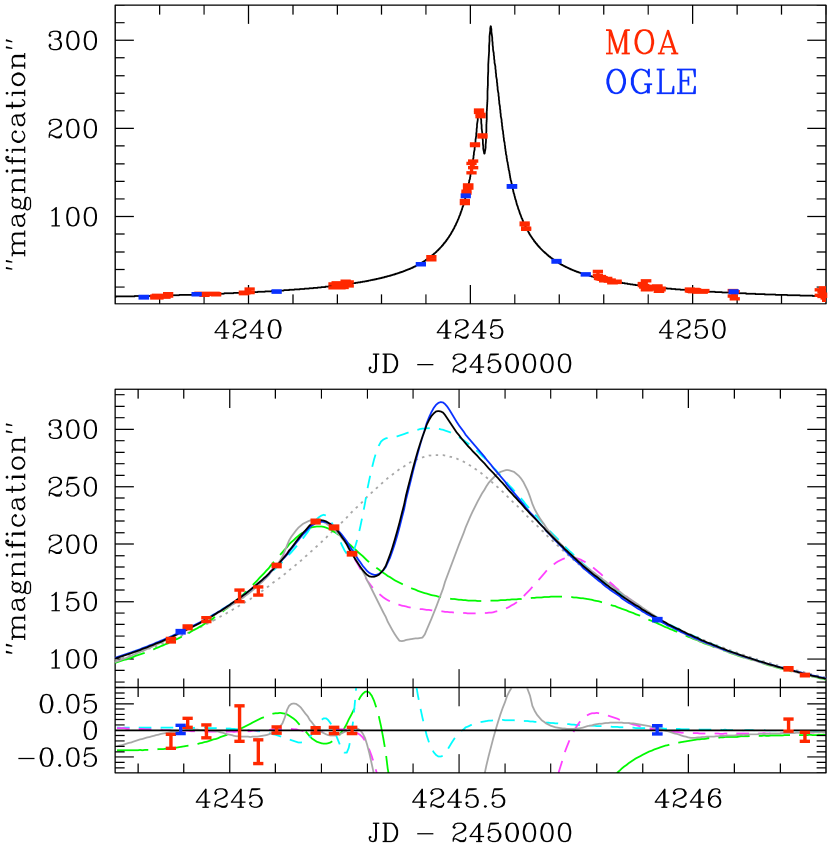
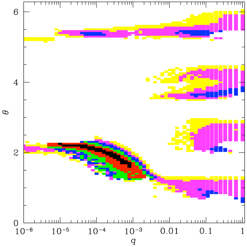
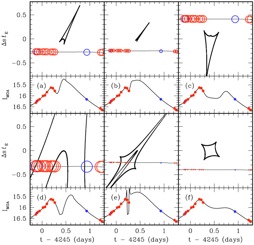
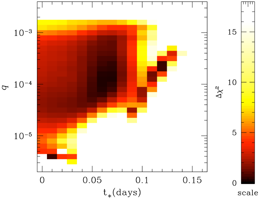
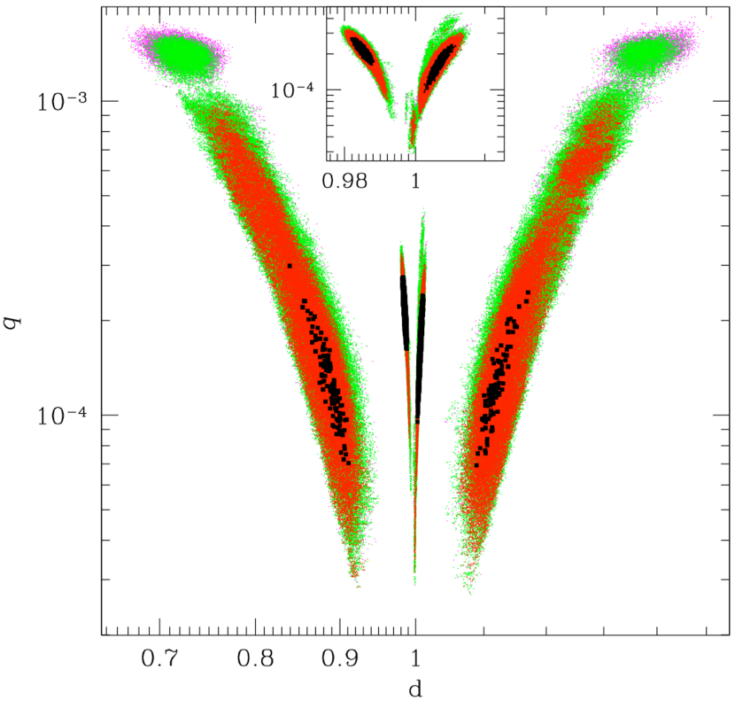
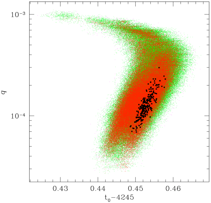
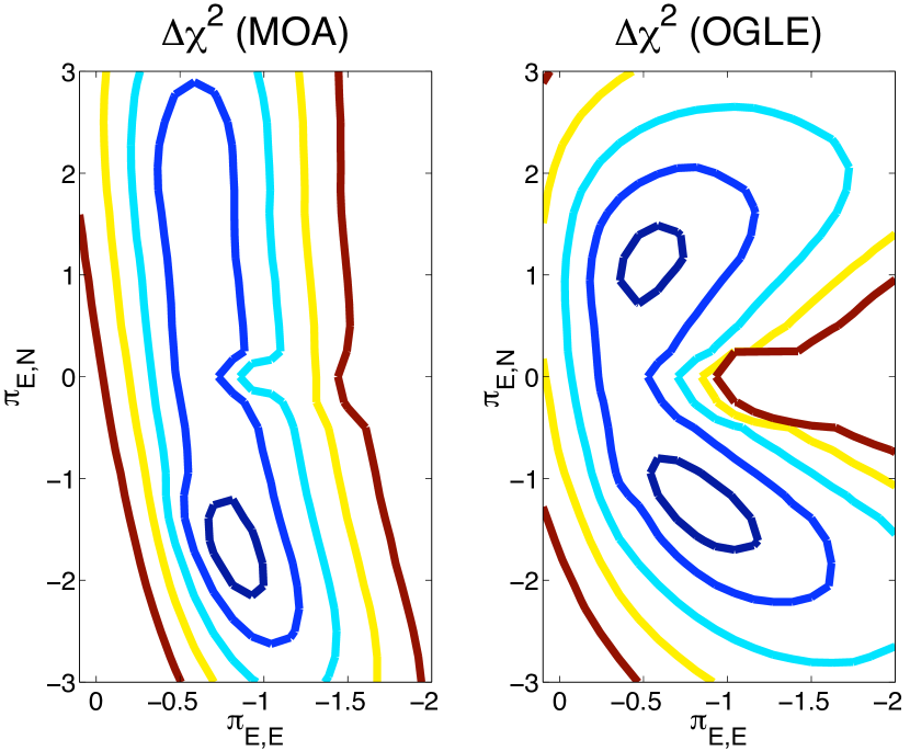
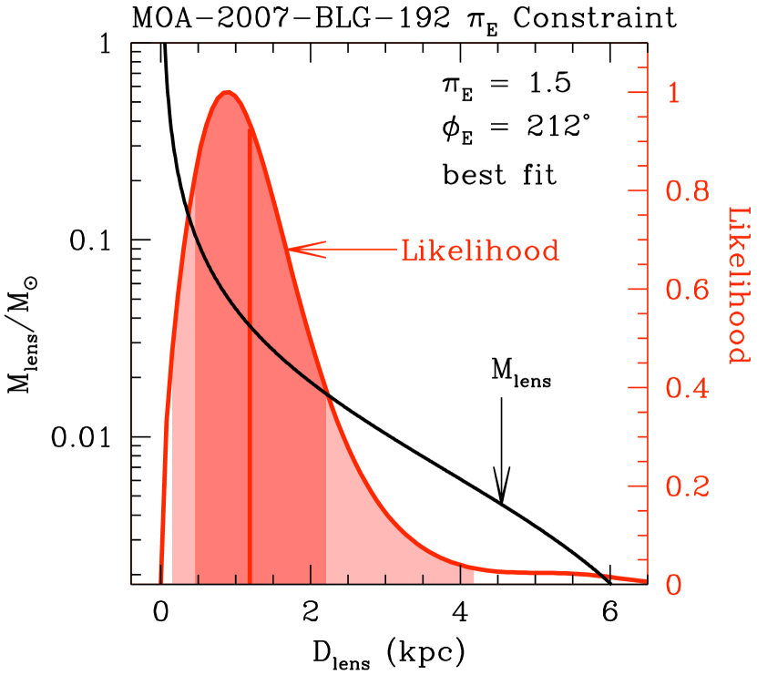
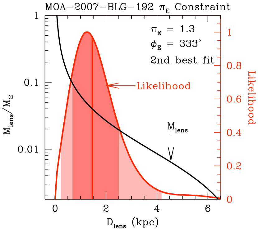
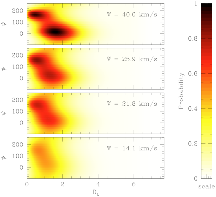
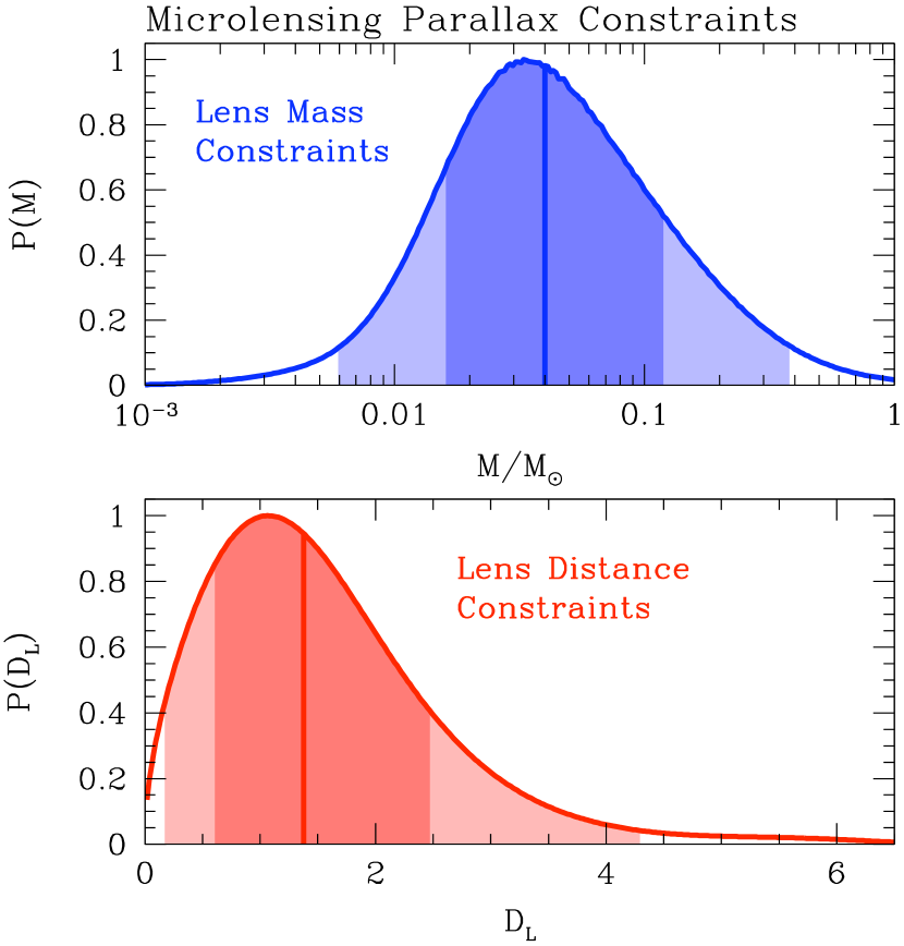
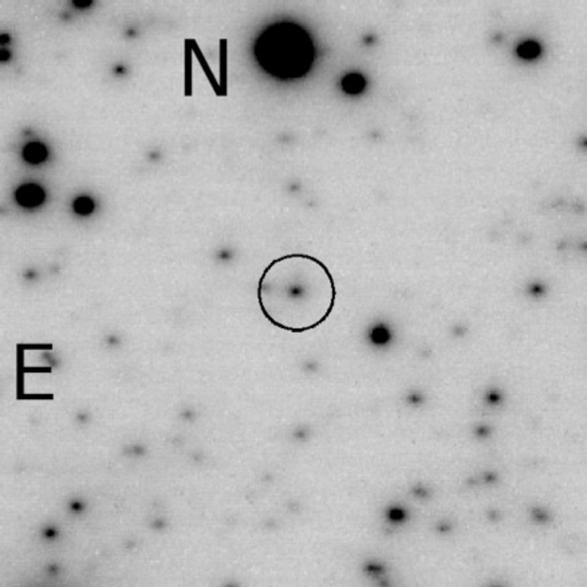
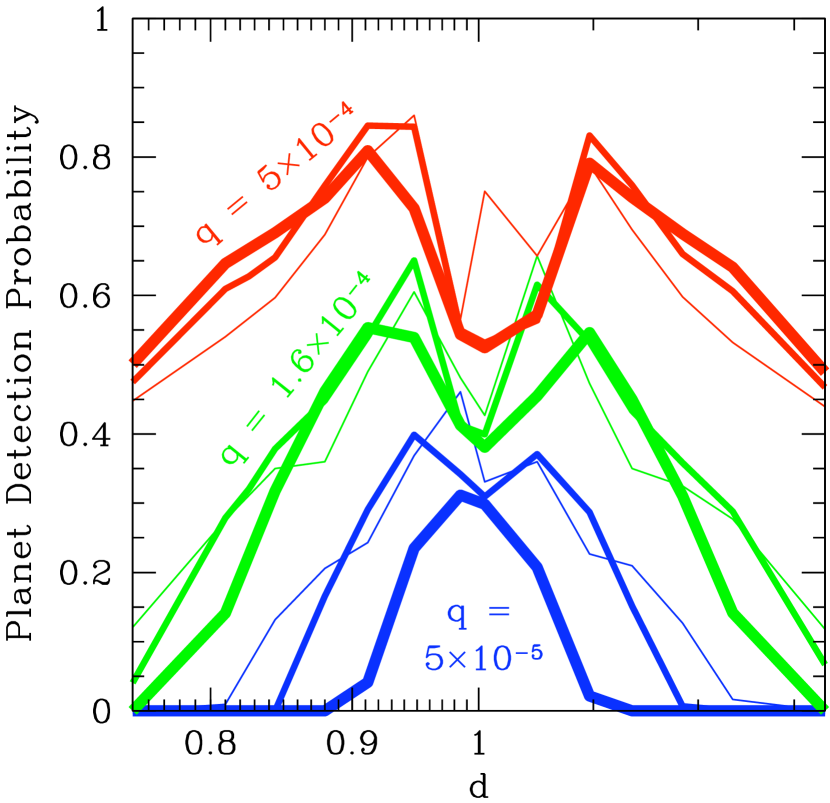
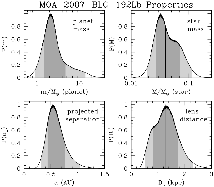
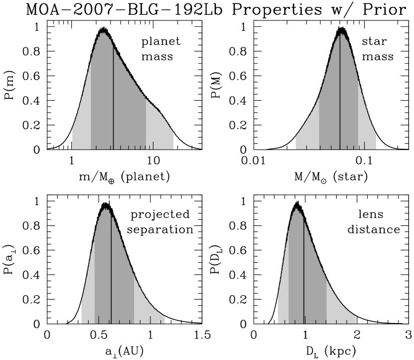
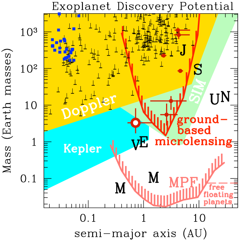
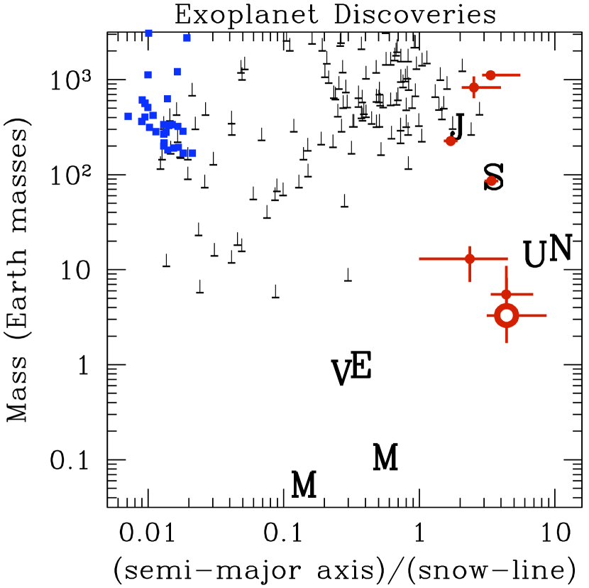
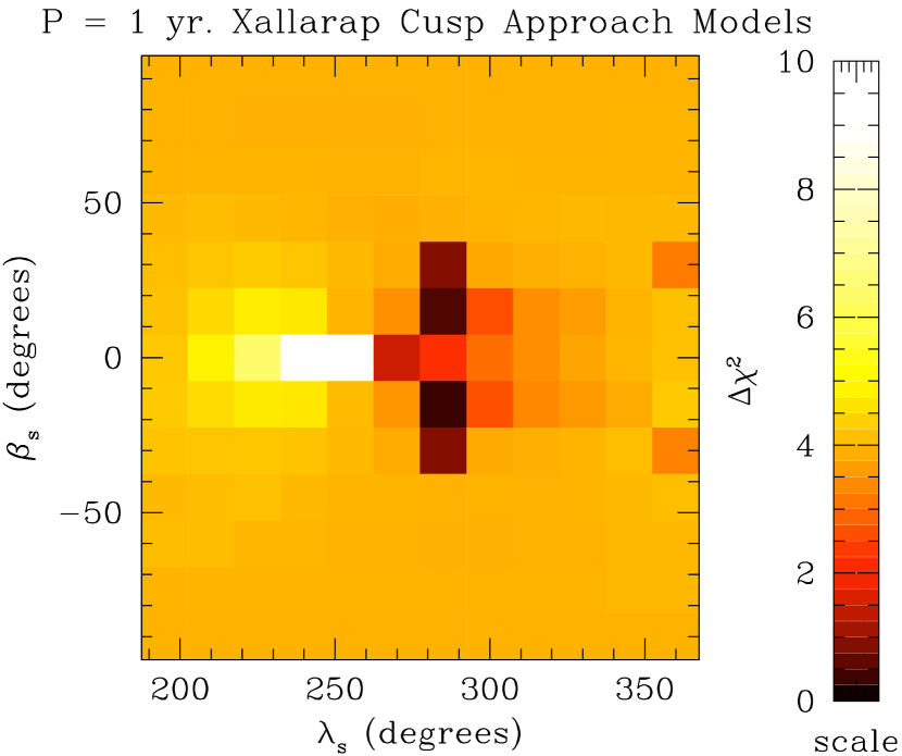
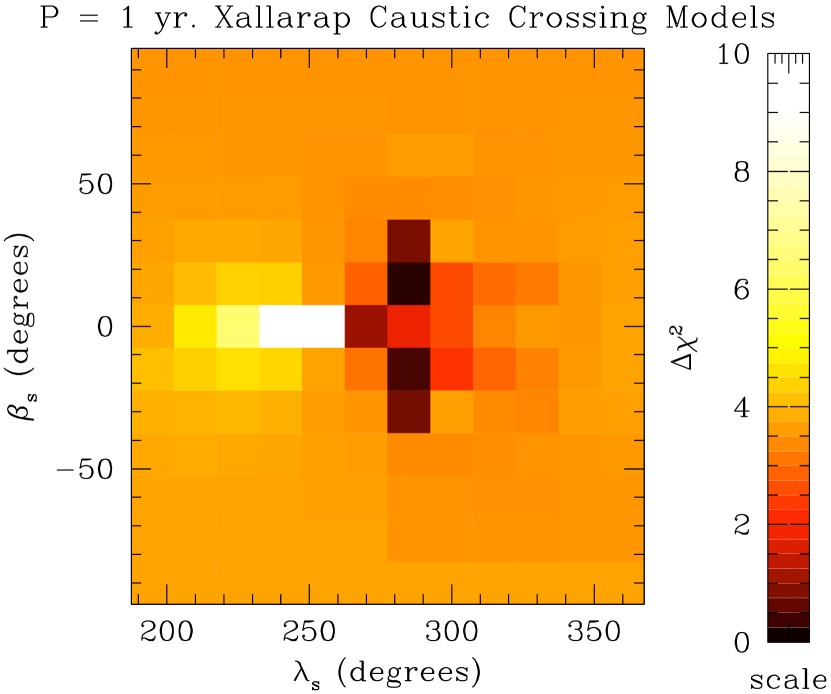
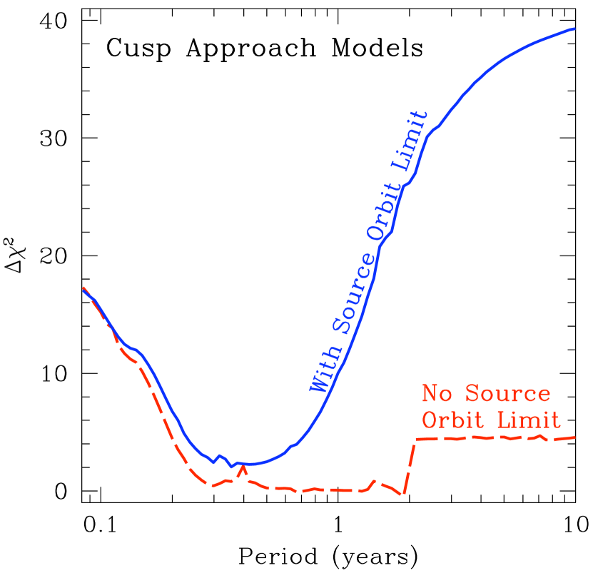
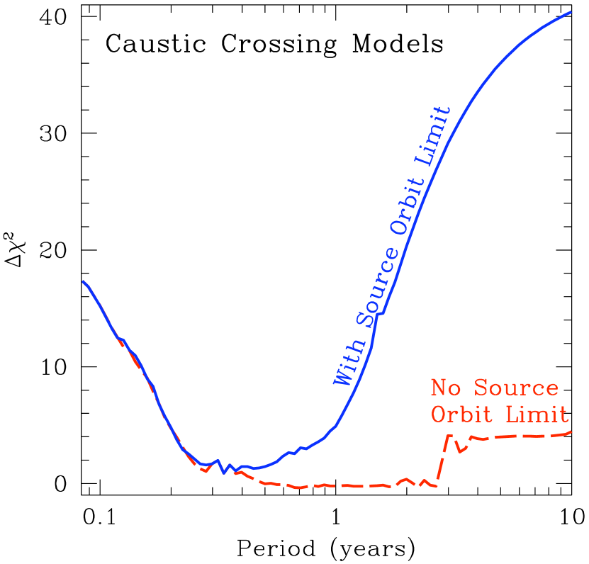
| Fit | |||||||||||
|---|---|---|---|---|---|---|---|---|---|---|---|
| A | 1115.52 | 75.0 | 5.453 | -0.00364 | 0.881 | 0.067 | 21.49 | 1.54 | |||
| B | 1115.46 | 74.5 | 5.453 | -0.00360 | 1.120 | 0.064 | 21.48 | 1.52 | |||
| C | 1116.32 | 73.4 | 5.449 | 0.00381 | 0.874 | 0.062 | 21.47 | 1.43 | |||
| D | 1116.37 | 73.8 | 5.448 | 0.00372 | 1.120 | 0.063 | 21.48 | 1.53 | |||
| E | 1117.69 | 70.6 | 5.454 | -0.00390 | 0.879 | 0.063 | 21.43 | 1.17 | |||
| F | 1117.84 | 69.1 | 5.451 | -0.00420 | 1.152 | 0.068 | 21.40 | 1.20 | |||
| G | 1117.38 | 70.1 | 5.454 | 0.00395 | 0.885 | 0.069 | 21.41 | 1.29 | |||
| H | 1117.35 | 69.9 | 5.456 | 0.00404 | 1.134 | 0.069 | 21.41 | 1.21 | |||
| I | 1115.14 | 75.1 | 5.462 | -0.00433 | 0.985 | 0.117 | 21.49 | 1.60 | |||
| J | 1115.12 | 74.9 | 5.458 | -0.00420 | 1.007 | 0.114 | 21.49 | 1.59 | |||
| K | 1115.59 | 69.4 | 5.455 | 0.00490 | 0.984 | 0.117 | 21.41 | 1.50 | |||
| L | 1115.88 | 72.4 | 5.453 | 0.00442 | 1.006 | 0.111 | 21.46 | 1.52 | |||
| M | 1116.81 | 68.7 | 5.459 | -0.00483 | 0.985 | 0.116 | 21.39 | 1.30 | |||
| N | 1117.59 | 69.3 | 5.454 | -0.00452 | 1.005 | 0.111 | 21.41 | 1.23 | |||
| O | 1116.36 | 68.9 | 5.463 | 0.00476 | 0.985 | 0.117 | 21.39 | 1.34 | |||
| P | 1117.26 | 66.4 | 5.458 | 0.00475 | 1.006 | 0.113 | 21.35 | 1.29 |
Note. — This table shows the fit parameters for the 16 distinct planetary models for MOA-2007-BLG-192. days. and are the time and distance of the closest approach of the source to the lens center-of-mass. and are the planet:star mass ratio and separation, and is the angle between the source trajectory and the planet-star axis. is the best fit source magnitude, and and are the magnitude and angle of the microlensing parallax vector. The units for the Einstein radius crossing time, , the source radius crossing time, , and are days, and all other parameters are dimensionless.
| parameter | value | 2- range |
|---|---|---|
| 0.019– | ||
| 0.9– | ||
| AU | 0.32–AU | |
| kpc | 0.5–kpc | |
| 21.30–21.60 | ||
| 0.6– |
| parameter | value | 2- range |
|---|---|---|
| 0.024– | ||
| 1.0– | ||
| AU | 0.33–AU | |
| kpc | 0.5–kpc | |
| 21.31–21.61 | ||
| 0.5– |