Baryon acoustic signature in the clustering of density maxima
Abstract
We reexamine the two-point correlation of density maxima in Gaussian initial conditions. Spatial derivatives of the linear density correlation, which were ignored in the calculation of Bardeen et al. [Astrophys. J. , 304, 15 (1986)], are included in our analysis. These functions exhibit large oscillations around the sound horizon scale for generic CDM power spectra. We derive the exact leading-order expression for the correlation of density peaks and demonstrate the contribution of those spatial derivatives. In particular, we show that these functions can modify significantly the baryon acoustic signature of density maxima relative to that of the linear density field. The effect depends upon the exact value of the peak height, the filter shape and size, and the small-scale behaviour of the transfer function. In the CDM cosmology, for maxima identified in the density field smoothed at mass scale and with linear threshold height , the contrast of the BAO can be a few tens of percent larger than in the linear matter correlation. Overall, the BAO is amplified for and damped for . Density maxima thus behave quite differently than linearly biased tracers of the density field, whose acoustic signature is a simple scaled version of the linear baryon acoustic oscillation. We also calculate the mean streaming of peak pairs in the quasi-linear regime. We show that the leading-order 2-point correlation and pairwise velocity of density peaks are consistent with a nonlinear, local biasing relation involving gradients of the density field. Biasing will be an important issue in ascertaining how much of the enhancement of the BAO in the primeval correlation of density maxima propagates into the late-time clustering of galaxies.
I Introduction
Sound waves propagating in the primordial photon-baryon fluid imprint a oscillatory pattern in the anisotropies of the Cosmic Microwave Background (CMB) and in the matter distribution, whose characteristic length scale is the sound horizon at the recombination epoch baotheory . for the currently favoured cosmological models. While experiments have accurately measured this fundamental scale and its harmonic series in the temperature and polarisation power spectra of the CMB, this acoustic signature has recently been detected in the correlation function of galaxies Eisenstein et al. (2005); baoobs . There is also weak evidence for the baryon oscillations in the correlation function of clusters Estrada et al. (2008). In the 2-point correlation, the series of maxima and minima present in the power spectrum translates into a broad peak at the sound horizon scale. Since the latter can be accurately calibrated with CMB measurements, the baryon acoustic oscillations (BAO) have emerged as a very promising standard ruler for determining the angular diameter distance and Hubble parameter baoprobe . Measuring the BAO at different redshifts thus offers a potentially robust probe of the dark energy equation of state.
In linear theory, the amplitude of the baryon acoustic peak increases while its shape and contrast remain unchanged. However, the clustering of galaxies does not fully represent the primeval correlation. Mode-coupling, pairwise velocities and galaxy bias are expected to alter the position and shape of the acoustic peak and, therefore, bias the measurement 3dbias . The evolution of the acoustic pattern in the 2-point statistics of the matter, halo or galaxy distributions has been studied using both numerical simulations Meiksin et al. (1999); baosimu and analytic techniques based on the halo model or perturbation theory Jeong & Komatsu (2006); Schultz & White (2006); Guzik et al. (2007); Eisenstein et al. (2007); Smith et al. (2007); Matarrese & Pietroni (2007); Crocce & Scoccimarro (2008); Smith et al. (2008); Matsubara (2008); Matarrese & Pietroni (2008); Seo et al. (2008); JeongKomatsu2008 . Yet the results of these studies do not always agree and the impact of nonlinearities on the matter and galaxy power spectrum remains debatable. For instance, References Schultz & White (2006); Eisenstein et al. (2007) argue that any systematic shift (i.e. not related to random motions or biasing) must be less than the percent level owing to the particularly smooth power added by nonlinearities on those scale, and to the cancellation of the mean streaming of (linearly) biased tracers at first order. On the other hand, References Guzik et al. (2007); Smith et al. (2007); Crocce & Scoccimarro (2008); Smith et al. (2008) have shown that mode-coupling modifies the acoustic pattern in the correlation of dark matter and haloes, and generates a percent shift towards smaller scales. Despite their redshift dependence, these shifts appear to be predictable and could be removed from the data Seo et al. (2008).
There is a broad consensus regarding the shape of the acoustic peak. In light of the nonlinear gravitational evolution of matter fluctuations, it is sensible to expect a baryon acoustic peak less pronounced in the late-time clustering of galaxies than in the linear theory correlation. This can be shown to hold for any local transformation of the density field Eisenstein et al. (2007); Coles (1993); Scherrer & Weinberg (1998). Such biasing mechanisms do indeed predict a damping of the baryon acoustic features in the 2-point statistics of the galaxy distribution Meiksin et al. (1999); Seo & Eisenstein (2005); Smith et al. (2007). Galaxies, of course, form a discrete set of points but one commonly assumes them to be a Poisson sample of some continuous field. Still, the extent to which those models are an accurate approximation to the clustering of galaxies remains unclear. Notice also that a reconstruction of the primordial density field could significantly restore the original contrast of the acoustic oscillation Eisenstein et al. (2007).
The main objective of this paper is to demonstrate that the BAO in the correlation of tracers of the density field can be noticeably modified if we consider local biasing relations more sophisticated than local transformations of the density field Szalay (1988); Fry & Gaztañaga (1993). To this purpose, we will examine the clustering of density maxima in the initial cosmological density field. In this respect, we will assume that the initial fluctuations are described by Gaussian statistics. This assumption is remarkably well supported by measurements of the CMB and large-scale structures gaussianity ; wmap5 . Density peaks form a well-behaved point-process whose statistical properties depend not only on the underlying density field, but also on its first and second derivatives. Therefore, although the number of density maxima is modulated by large-scale fluctuations in the background, their clustering properties cannot be derived from a continuous field approach in which the peak overdensity would depend upon the value of the matter density only. Interestingly however, we shall see that, at large separations, the peak correlation and pairwise velocity are consistent with a nonlinear biasing relation involving gradients of the density field.
In a seminal paper, Bardeen, Bond, Kaiser & Szalay (hereafter BBKS) Bardeen et al. (1986) provided a compact expression for the average number density of peaks in a three-dimensional Gaussian random field, etc. Furthermore, they obtained a large-scale approximation for the correlation function of peaks which, at large threshold height, tends toward the correlation of overdense regions Kaiser (1984); Politzer & Wise (1984); Jensen & Szalay (1986) as it should be. However, BBKS determined the correlation function of density maxima only in the limit where derivatives of the 2-point function of the density field can be ignored. As we will see below, these correlations can greatly influence the large-scale correlation of density maxima for generic Cold Dark Matter (CDM) power spectra. It is also worth noticing that the statistics of Gaussian random fields in a cosmological context has received some attention in the literature Doroshkevich (1970); Hoffman & Shaham (1985); Peacock & Heavens (1985); Coles (1989); Lumsden, Heavens & Peacock (1989). Some of these results have been applied to the mass function and correlation of rich clusters for example Kaiser & Davis (1985); Otto et al. (1986); Cen (1998). The present work mainly follows the analytic study of BBKS, and the lines discussed in Desjacques (2007); Desjacques & Smith (2008), where 2-point statistics of the linear tidal shear are investigated. We refer the reader to Adler & Taylor (2007) for a rigorous introduction to the statistics of maxima of Gaussian random fields.
The paper is organised as follows. Section II introduces a number of useful variables and correlation functions. Section III is devoted to the derivation of the leading order expression for the large-scale asymptotics of the peak correlation. Our result can be thought as arising from a specific type of nonlinear local biasing relation including second spatial derivatives of the density field. In Sec. IV, we explore the impact of these derivatives on the amplitude and shape of the correlation of density maxima. Our attention focuses on the baryon oscillation, across which the amplitude of the linear matter correlation varies abruptly. It is shown that the BAO of density maxima can be amplified relative to that of the matter distribution. Section V deals with the peak pairwise velocity. Its leading order contribution is found to be consistent with the nonlinear local bias relation inferred from the 2-point correlation of peaks. A final section summarises our results.
II Properties of cosmological Gaussian density fields
We review some general properties of Gaussian random fields and provide explicit expressions for the correlations of the density and its lowest derivatives. We show that the latter are not always negligible in CDM cosmologies.
II.1 Useful definitions
We will assume a CDM cosmology with normalisation amplitude , and spectral index wmap5 . The matter transfer function is computed using publicly available Boltzmann codes boltzmann . The position of the BAO in the linear matter correlation function is close to .
Let q designate the Lagrangian coordinate. We are interested in the three-dimensional density field and its first and second derivatives. It is more convenient to work with the normalised variables , and , where the are the spectral moments of the matter power spectrum,
| (1) |
denotes the dimensionless power spectrum of the density field smoothed on scale with a spherically symmetric window .
The best choice of smoothing is open to debate. Among the popular window functions, the top hat filter is compactly supported and has a straightforward interpretation within the spherical collapse model. Notwithstanding this, oscillations that arise in Fourier space do not lead to well defined spectral moments with for CDM power spectra. This can be understood by examining the high- tail of the CDM transfer function. Neglecting the baryon thermal pressure on scale less than the Jeans length, the small-scale matter transfer function behaves as Bardeen et al. (1986); tksmalltail , which clearly leads to divergences when the integer is larger than one. By contrast, a Gaussian window function ensures the convergence of all the spectral moments for any realistic matter power spectra. Consequently, we shall mostly rely on the Gaussian filter throughout this paper, although the top hat filter will also be considered briefly in Sec. IV. Note that a Gaussian filter of characteristic width encloses a mass a few times larger than that encompassed by a top hat filter of identical smoothing radius.
Following BBKS, we also introduce the parameters and for subsequent use. The spectral width reflects the range over which is large, while characterises the radius of peaks. For the special case of a powerlaw power spectrum with Gaussian filtering on scale , these parameters are given by and . For CDM power spectra, when the smoothing length varies over the range .
II.2 Correlation of the density and its derivatives
Calculating the 2-point correlation of density peaks requires knowledge of the auto- and cross-correlations of the various fields. These objects can be decomposed into components with definite transformation properties under rotations. Statistical isotropy and symmetry implies that, in position space, the most general ansatz for the isotropic sector of the 2-point correlations of these fields reads
| (2) | |||||||
where is the Lagrangian separation, and the functions , , , and depend on only. We emphasise that these correlation functions transform as scalar under rotations. Note also that these expressions are valid for any arbitrary random field. For a cosmological Gaussian density field however, these functions can be summarised as follows :
| (3) | |||||
are spherical Bessel functions of the first kind. In the limit , all the correlation functions vanish but , and , which tend towards 1, 1/3 and 1/15, respectively. Averaging over the direction of the separation vector thus yields
| (4) | |||||
for the covariances of the fields and , where we have defined
| (5) | |||||
The angular average of the other correlation functions vanishes, except that of the density correlation of course.
and can be expressed in terms of the derivatives of the density correlation using relations like etc. For a density correlation that falls off as a powerlaw , and decay as and , respectively. This derivation assumes a powerlaw power spectrum with a fair amount of power at short wavenumbers. Hence, as recognised in BBKS, neglecting the derivatives of the density correlation should be a reasonable approximation when .
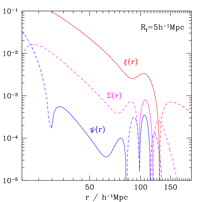
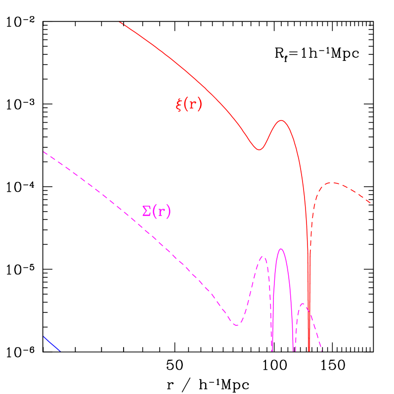
This simple argument may not hold for CDM cosmologies since the index is a smooth function of the separation . Namely, it is when , and increases to attain a value of the order of unity on scale . For illustration purpose, the functions , and are plotted in Figures 1 and 2 for the CDM cosmology considered here. The filtering length is and , respectively (The reason for choosing these values will become apparent below). Retaining only the density correlation appears to be a good approximation on scales larger than a few smoothing radii. However, the relative amplitude of the cross-correlations strongly depends upon the filtering scale. Namely, both and increase relative to with increasing smoothing length. Yet another striking feature of Figures 1 and 2 is the oscillatory behaviour of and . The large oscillations are caused by rapid changes in the linear matter correlation across the baryon acoustic peak. Notice that both and are positive at distances . On these scales, when , reaches to 3 per cent of the density correlation while is negligible. At the large smoothing length however, they nearly reach 20 and 10 per cent of the density correlation, respectively.
These results suggest that, for generic CDM power spectra, the derivatives of the density correlation could have a significant impact on the correlation of density maxima, especially in the vicinity of the baryon acoustic feature. This motivates the calculation presented in the next Section.
III Correlation of density maxima
Owing to the constraints on the derivatives of the density field, calculating the -point correlation function of peaks requires performing integration over a joint probability distribution in 10 variables. Therefore, even the evaluation of the 2-point correlation of density maxima proves difficult. Here, we derive the leading order expression that includes, in addition to the linear matter correlation , the contribution of the angular average functions and . We also show that the large-scale asymptotics of the peak correlation can be thought as arising from a specific type of nonlinear biasing relation involving second derivatives of the density field.
III.1 The Kac-Rice formula
As shown in BBKS for instance, the correlation of density extrema (maxima, minima and saddle points) can be entirely expressed in terms of and its derivatives, and . In the neighbourhood of an extremum, the first derivative is approximately
| (6) |
Using the properties of the Dirac delta, the number density of extrema can be written as
| (7) |
provided that the Hessian is invertible. The delta function ensures that all the extrema are included. In this paper however, we are interested in counting the maxima solely. Consequently, we further have to require be negative definite at the extremum position . Note that, later, we will also restrict the set to those maxima with a certain threshold height. The average number density of maxima eventually reads
| (8) |
This expression, known as the Kac-Rice formula Kac (1943); Rice (1954); Belyaev (1967); Cline et al. (1987); Adler & Taylor (2007), holds for arbitrary smooth random fields. In the general case of a random field in dimensions, it is trivial to show that the mean density of maxima scales as .
The 2-point correlation function of density peak is defined such that
| (9) |
is the joint probability that a density maxima is in a volume about each . Let be the diagonal matrix of entries where is the non-increasing sequence of eigenvalues of the symmetric matrix . The condition that the extrema are maxima implies . Therefore, the correlation function of peaks is given by
where, for shorthand convenience, subscripts denote quantities evaluated at different Lagrangian positions, and is the usual Lebesgue measure on the six-dimensional space of symmetric matrices. Here and henceforth designates the Heaviside step-function, i.e. for and zero otherwise.
III.2 Two-point probability distribution
The joint probability distribution of the density fields together with its first and second derivatives, , is given by a multivariate Gaussian whose covariance matrix has 20 dimensions. This matrix may be partitioned into four block matrices, in the top left corner and bottom right corners, and its transpose in the bottom left and top right corners, respectively. The components , of the ten-dimensional vector symbolise the entries of . To emphasise that the entries transform as a tensor under rotation, we shall also label them as the matrix in what follows.
The matrices and can be further decomposed into block sub-matrices of size 4 and 6,
| (11) |
Unlike the which describe the covariances at a single position, the matrices generally are functions of the separation vector r. Using the harmonic decomposition of the tensor products , they can be written as
| (12) |
are spherical harmonics and are matrices which satisfy . Only multipoles up to appear in the harmonic decomposition since the correlations given in eq. (II.2) involve products of up to four unit vectors . The monopole terms are
| (15) | |||||
| (18) | |||||
| (21) |
where
| (22) |
is the identity matrix and etc. The matrices are readily obtained as . An explicit computation of the higher multipole matrices is unnecessary here as we confine the calculation to the monopole contribution.
It is important to note that the joint density preserves its functional form under the action of the rotation group SO(3). However, in a given frame of reference, does change when moves on the unit sphere. Does this mean that truly depends on the direction of the separation vector r ? No, as it should be clear from eq. (III.1) where the volume measure is a rotational invariant. More precisely, the volume element can be cast into the form
| (23) |
where the s are, as before, the three ordered eigenvalues of , and is the Vandermonde determinant. is the Haar measure (for the Euler angles for example) on the group SO(3) normalised to . The peak correlation thus is proportional to
| (24) |
where the integral runs over the two SO(3) manifolds that define the orientation of the principal frames of and relative to the frame of reference. Alternatively, we can choose the coordinate system such that the coordinate axes are aligned with the principal axes of . In this new coordinate frame, the above integral becomes
| (25) |
where is an orthogonal matrix that defines the orientation of the eigenvectors of relative to those of . This demonstrates that only the monopole component of contributes to the peak correlation function. Therefore, is invariant under rotations of the coordinate system, namely, it is a function of the separation only.
III.3 Large scale asymptotics
To obtain the correlation function of peak, we need first to calculate the 2-point probability distribution function averaged over the unit sphere for the variables ,
| (26) |
In the large-distance limit (), the cross-correlation matrix is small when compared to the zero-point contribution , e.g. . Following Desjacques (2007); Desjacques & Smith (2008), the quadratic form which appears in the probability distribution ,
| (27) |
where is the determinant of the covariance matrix , can be computed easily using Schur’s identities. Expanding the exponential in the small perturbation yields, to first order,
| (28) |
where the quadratic form can be recast as
| (29) |
in agreement with the results of BBKS. The calculation of is tedious but straightforward. Fortunately, only the monopole terms survive after averaging over the directions . After further simplification, the result can be reduced to the following compact expression :
The invariance under rotation requires that be a symmetric function of the eigenvalues, and thus a function of ,
Since the above expression depends only upon the relative orientation of the two principal axes frames of and (through the presence of ), we choose a coordinate system whose axes are aligned with the principal frame of . With this choice of coordinate, we define and , where is an orthogonal matrix that defines the relative orientation of the eigenvectors of . and are the diagonal matrices consisting of the three ordered eigenvalues and of the Hessian . The properties of the trace imply that , (and similarly for ), while the term depends explicitely on the rotation matrix .
The integral over the SO(3) manifold that describes the orientation of the orthonormal triad of is immediate. The result is (and not ) as we don’t care whether the axes are directed towards the positive or negative direction. The integral over the second SO(3) manifold involves
| (31) |
and yields cancellation of the first term in the right-hand side of eq. (25). To integrate over the eigenvalues of and , we transform to the new set of variables , where
| (32) |
The variables are similarly defined in terms of the . We will henceforth refer to as the peak curvature.
Our choice of ordering imposes the constraints and . The condition that the density extrema be maxima, i.e. all three eigenvalues of the Hessian are negative, translates into . Another condition, , should also be applied if one is interested in selecting maxima with positive threshold height.
For shorthand convenience, and to facilitate the comparison with the calculation of BBKS, we introduce the auxiliary function
measures the degree of asphericity expected for a peak and can be used to determine the probability distribution of ellipticity and prolateness Bardeen et al. (1986). It scales as in the limit .
III.4 The peak correlation
For sake of generality, we will present results for the cross-correlation between two populations of density maxima identified at smoothing scale . However, we shall focus shortly on the auto-correlation ( and ), which is more directly related to the clustering properties of dark matter haloes of a given mass or galaxies and clusters of a given luminosity spanning a narrow redshift range. It may also be interesting to work out the correlation of peaks with a fixed height but identified at smoothing radii , which can be thought as mimicking the statistical properties of haloes above a given mass. However, we will not consider this correlation here since it requires a solution to the cloud-in-cloud problem Bond et al. (1991) at the location of density maxima.
Let hereafter denote the differential density of peaks in the range to . The expectation value of the product of the local peak densities that appears in eq. (9) is then
| (34) |
where
is equation (25) averaged over the relative orientation of the frames spanned by the eigenvectors of and . depends on the separation through the correlation functions , and only. Furthermore, the quadratic form simply is
| (36) |
in the variables (32).
The integration over the variables and is lengthy but straightforward. We refer the reader to BBKS for the details since the calculation now proceeds along similar lines. Let us mention that the allowed domain of integration is the interior of a triangle bounded by the points , and . As shown in BBKS, the differential density of peak of height can be cast into the form
| (37) |
where is the zeroth moment of the peak curvature . Higher moments are written in explicit compact form as
| (38) |
Using this result, the correlation of peaks can be rearranged as follows :
| (39) |
For sake of completeness,
as demonstrated in BBKS, who noted also that the asymptotic limits of this function include a cancellation to eighth order at small , and the law expected for density maxima at large .
The integration over must generally be done numerically. It is worth noticing that, while the exponential decays rapidly to zero, are monotonically and rapidly rising. As a result, the functions are sharply peaked around their maximum. For large values of , we find that and asymptote to
| (41) | |||||
The coefficients , and are obtained from the asymptotic expansion of the Error function that appears in eq. (III.4). We have explicitly
| (42) |
The rest of the calculation is easily accomplished. The 2-point correlation function of peaks eventually reads
where we have introduced the mean curvature . Also, the notation is such that . The function is accurately fitted by eq. (4.4) of BBKS, which is constructed to match the asymptotic large expansions of and given in eq. (III.4). In the special case , the 2-point correlation of peaks simplifies to
| (44) |
where the bias functions , and are
| (45) |
The sign convention is chosen such that all three bias parameters are positive when . Notice that is precisely the amplification factor found by BBKS when derivatives of the density correlation function are neglected.
Equation (44), which holds for any value of the peak height and the smoothing length , is the main result of this Section. It describes the asymptotic behaviour of the peak correlation function in the limit where the correlation functions , and are much less than unity.
III.5 The bias parameters
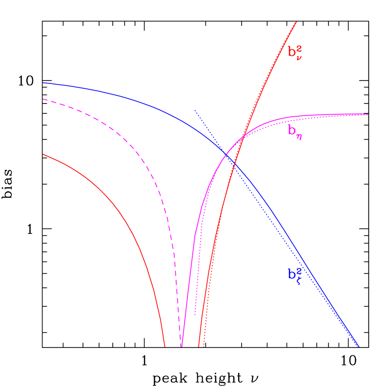
To gain some insight into the behaviour of the peak correlation function , we have plotted in Fig. 3 the biasing parameters , and as a function of the peak height. Again, the density field is smoothed on scale with a Gaussian filter. The dotted curves show the following large approximations,
| (46) |
obtained from the asymptotic expansions of and (eq. III.4). They provide a good match to the bias parameters when the peak height is larger than . As we can see, tends towards the constant value of 6 when . Moreover, for a threshold height less than unity, is negative and of absolute magnitude larger than . This is also true in the intermediate region . For these threshold heights, both and vanish while the bias parameter is of the order of a few. Consequently, the correlation of density maxima, albeit weak for peak heights of the order of unity, never cancels out. Overall, retaining the density correlation solely is not a reasonable approximation when the peak height does not exceed . Although the exact value of the bias parameters changes somewhat with the smoothing scale , their global behaviour varies little as weakly depends on the filtering scale. Therefore, the above statements hold regardless of the exact amount of smoothing.
III.6 Peak biasing : nonlinear and local ?
Equation (44) clearly differs from the linear, local relation that would be expected if the peak overdensity were related to the underlying density field through the linear mapping . However, it is worth noticing that eq. (44) is compatible with a nonlinear, local, deterministic biasing relation involving a differential operator. Namely, it can be explicitly checked that
| (47) |
where , leads to the correlation function (44). This demonstrates that, at large distances, can be thought as arising from a specific case of nonlinear local bias. We will see later (Sec. V) that this local mapping is also consistent with the peak pairwise velocity at first order.
To make connection with the formalism introduced by Fry & Gaztañaga (1993), we may conceive of a Taylor series
| (48) |
to describe the properties of the peak distribution at all separations and filtering scales. An expansion of the peak correlation beyond leading order will be required to determine the values of the and when . Higher derivatives of the density field may also contribute to this general expression. However, (nonlocal) integrals of the linear density correlation are expected only in the evolved matter distribution when the non-Gaussianity induced by gravitational clustering is significant.
Finally, it is worth noticing that, upon Fourier transformation, the peak power spectrum reads
| (49) |
where and is the power spectrum of the smoothed density field. The exact amount of scale-dependence induced by the nonlinear bias depends upon the exact value of and . We defer a thorough investigation of this effect to a future work.
IV Clustering of density peaks in Gaussian Initial Conditions
After a brief discussion on the peak-background split, we focus on the acoustic signature in the 2-point correlation of density maxima. We examine how the baryon acoustic oscillation changes with the filtering, the threshold height and the small-scale behaviour of the transfer function. We find that the extra contributions and to the linear relation can boost significantly the contrast of the acoustic peak.
IV.1 Filtering scale and peak height
The peak height and the filtering radius could in principle be treated as two independent variables. However, in order to make as much connection with dark matter haloes (and, to a lesser extent, galaxies) as possible, we will follow the Press-Schechter prescription Press & Schechter (1974) which is based on the critical density criterion issued from the spherical collapse dynamics Gunn & Gott (1972). Namely, we assume that density maxima with peak height identified in the primeval density field smoothed at scale are related to dark matter haloes of mass collapsing at redshift . Moreover, we will only present results at redshift , at which the linear critical density for (spherical) collapse is , and the characteristic mass for clustering is . While there is a direct correspondence between the massive cluster-sized haloes in the evolved density field and the largest maxima of the initial density field, it is unclear the extent to which galaxy-sized haloes trace the initial density maxima galaxypeak . For this reason, we will only consider mass scales in the range or, equivalently, a smoothing radius .
We note that the spherical infall model provides a local approximation to the collapse of a perturbation. However, in the Press-Schechter approach, it is applied to random points in space and leads to linear local biasing at large scales Mo & White (1996); Sheth & Tormen (1999) while, in the present work, it is applied to density maxima and leads to the specific type of nonlinear local biasing exemplified by eq. (47).
IV.2 Peak-background split and the halo multiplicity function
Before illustrating the impact of derivatives of the density field on the baryon acoustic signature, we note that, in the limit , the peak correlation is amplified by an effective bias which is significantly smaller than the value derived for thresholded regions Kaiser (1984). As recognised in BBKS, this difference arises from the correlation between the peak height and the peak curvature . More precisely, in the spherical infall model, the linear Lagrangian bias of high density peaks that are collapsing at redshift evaluates to
| (50) |
in the limit . This should be compared to the expression derived in Mo & White (1996); Cole & Kaiser (1989) from the Press-Schechter formalism Press & Schechter (1974); Bond et al. (1991),
| (51) |
In this second approach, the clustering of haloes is described by the properties of regions above a given density threshold. In both cases however, the Kaiser limit is recovered. This, however, does not apply to the bias factor derived by Sheth & Tormen (1999) using the ellipsoidal collapse,
| (52) |
where . Assuming the peak-background split holds Kaiser (1984), these various bias parameters predict multiplicity functions Bond et al. (1991) that have quite a different behaviour in the limit of large threshold heights. In particular, the Sheth-Tormen (ST) multiplicity function is proportional to Sheth & Tormen (2002), and exponentially deviates from the scaling inferred from and , which is and , respectively. It is worth emphasising that the factor was essentially determined by the number of massive haloes in the GIF simulations Kauffmann et al. (1999) and, therefore, is not a direct outcome of the ellipsoidal collapse dynamics. In fact, there is no compelling theoretical reason for a halo mass function whose high-mass end deviates exponentially from the scaling . Furthermore, recent lines of evidence suggest that the high-mass tail, while being above the Press-Schechter (PS) mass function Press & Schechter (1974), may depart from the Sheth-Tormen scaling highmassend .
In our opinion, it is likely that the true multiplicity function scales as in the limit of large . This would lead to a different parametrisation of the halo bias and mass function. Given the lack of a convincing physical description of these quantities, one may, for instance, consider a phenomenological bias of the form
| (53) |
which, for a peak-background split, leads to a multiplicity function
| (54) |
For and (which guarantees in the limit ), the biasing (53) closely follows the peak scaling eq. (50) at large mass and, simultaneously, exhibits an upturn at low mass. Unfortunately, such a bias cannot be derived from an excursion set approach (upon which PS and ST are based), where invariably. This issue, which lies beyond the scope of the present paper, will be examined in a separate paper.
IV.3 Baryon acoustic signature
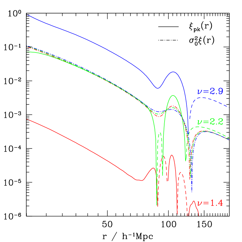
We now turn to the behaviour of the peak correlation function. is shown in Fig. 4 for a filtering length , 4 and . The mass enclosed in the Gaussian window thus is , and , respectively. To illustrate, we have adopted a peak height such that , 2.1 and 2.9, respectively. In the spherical infall dynamics, a top hat overdensity enclosing a similar amount of mass would collapse at redshift . Furthermore, the density correlation is also shown for comparison as the dotted curve.
The three correlations considered here exhibit a very different behaviour that reflects the strong dependence of the bias factors , and on the threshold height (see Sec. III.5). In particular, we find , 0.847 and 1.771 with increasing smoothing radius. As a result, for , the contribution of the term dominates the others and strongly suppresses the amplitude of relative to that of the density correlation. This term has the sign of and features several oscillations across the BAO scale (see Figures 1 and 2). However, for peaks of threshold height identified at smoothing scale , merely contributes to decrease the level of the minimum at distance . Interestingly, the term boosts significantly the contrast of the acoustic peak. This effect is still present, albeit weaker, for and . We also note that zero-crossings of do not generally coincide with those of , in agreement with numerical studies of the clustering of density maxima Coles (1989); Lumsden, Heavens & Peacock (1989).
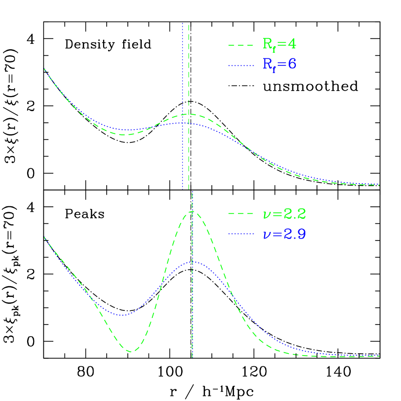
Fig. 5 further illustrates the sharpening of the acoustic peak due to correlations among derivatives of the density field. The density and the peak correlations are compared in the neighbourhood of the acoustic feature for the smoothing radii and considered above. To emphasise the contrast of the acoustic peak, all the correlations have been rescaled such that, at a distance , their amplitude is equal to 3. Fig. 5 nicely demonstrates the large impact of , which fully restores the acoustic signature of otherwise smeared out by the large filtering. The contrast of the acoustic peak can even be enhanced relative to that of the unsmoothed () linear density correlation (dotted-dashed line). The effect is strongest for the density peaks identified at the smaller smoothing, . For these maxima, the difference between the height of the (negative) minimum at and the maximum at is twice as large as in the linear density correlation. The enhancement is somewhat smaller, roughly 20 per cent, for the peaks at the filtering scale . This shows that density maxima behave rather differently than linearly biased tracers of the density field, whose acoustic signature cannot be larger than that of the linear matter correlation Eisenstein et al. (2007).
We now concentrate on the vertical lines which indicate the position of the local maximum. On the one hand, the top panel shows that smoothing in the density correlation generates a shift towards smaller scales, because the acoustic feature is not quite symmetric around its maximum Smith et al. (2007). On the other hand, the presence of in the peak correlation acts in the opposite sense and compensates for the shift induced by the smoothing. We find the maximum to be close to its linear value in both cases. More precisely, there is a small shift of per cent towards larger scales.
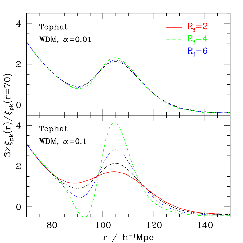
IV.4 Sensitivity to the filter shape and the transfer function
As discussed in BBKS, the filtering of the density field is an essential operation for power spectra covering a wide range of wavenumbers. However, the optimal choice of filter is disputable. Furthermore, the (analytic) properties of the filtered density field can depend significantly upon the amount of power in small-scale fluctuations. It is, therefore, important to assess the influence of the smoothing operation and the small-scale transfer function on the baryon acoustic signature in the correlation of density peaks.
To this purpose, we have repeated the numerical calculation of using a top hat filter. To avoid divergence of the spectral moments and the correlation functions, we have introduced a high- cutoff whose functional form is motivated by the damping of fluctuations due to the free streaming of the dark matter particle(s). So far, we have considered a CDM cosmology in which the velocity dispersion of the dark matter particle is negligible. By contrast, in Warm Dark Matter (WDM) cosmologies, the dark matter candidate(s) can suppress the matter power spectrum on galaxy scales Bond et al. (1980). The latter can be approximated as , where the transfer function that accounts for the free-streaming cutoff has the form tkwdm
| (55) |
Here, and depends upon the properties of the dark matter particles. Typically, for thermal relics of mass .
In spite of its compactness, the top hat filter has some inconvenient. Firstly, because of its slowly decaying tail, it produces a density field that is not differentiable for generic CDM power spectra Bond et al. (1991). Secondly, it is good at discriminating peaks from the background field so long as the height of the latter is small, namely, when the background field is uncorrelated over scales comparable to the filtering length. By contrast, the Gaussian filter is less sensitive to high frequencies and thus fares better at picking up smoother objects. Indeed, the “true” filter may lie between these two extremes Dalal et al. (2008). Notice that the sharp -space window will not be considered here as it leads to undesirable oscillations at all separations.
Fig. 6 shows the baryon acoustic peak in the correlation of density maxima for the smoothing radii used in Fig. 4 and 5. Note, however, that the filter mass scale is now roughly four times smaller than with the Gaussian window. The peak correlation is plotted for two values of the free-streaming cutoff, and 0.1 (top and bottom panels). Also shown in both panels for comparison is the linear matter correlation (dotted-dashed line). At smoothing length and , the enhancement of the acoustic peak is very significant for while, for , it is only 10-20 per cent. The main reason is a sharper power spectrum, which leads to a larger contribution of the correlations and to . At for instance, the spectral width is and 0.26 for and 0.01, respectively. This difference mostly arises because of the second spectral moment, which increases from to 0.76 upon the decrease in the free-streaming scale. Yet another interesting feature of Fig. 6 is the rather broad acoustic peak at filtering scale (see bottom panel), for which . This broadening follows from the fact that is negative at that value of threshold height. As a consequence, the oscillatory pattern of across the BAO (see Figures 1 and 2) smears out the acoustic feature in . As seen from Fig. 3, this damping always occurs at sufficiently low values of the threshold height, regardless of the filtering length. It should also be noted that, unlike the correlation of density maxima, the BAO in the smoothed linear matter correlation is weakly insensitive to the small-scale behaviour of the power spectrum. In however, the BAO acquires an extra dependence upon the high- tail of the transfer function through the correlation functions and .
To summarise,
-
•
Both and contribute to the correlation of density maxima and can affect the shape of the baryon acoustic signature for peak heights .
-
•
makes a significant contribution only in the range , where and are much less than unity.
-
•
The contribution of increases with the spectral width . At constant filtering length, it increases with the amount of power suppression due to the small scale free streaming.
-
•
is positive (negative) for (). As a result, the baryon acoustic peak is generally enhanced in when , and damped out when .
These results depend upon the exact shape of the filter and the transfer function. Clearly however, the effect cannot be reduced to a simple rescaling of the linear matter correlation. This is due to the peculiar type of nonlinear local biasing, eq. (47), which involves the Laplacian of the density field.
V Pairwise velocity of density maxima
Thus far, we have explored the BAO signature in the correlation of maxima of the primordial density field. However, pairwise motions caused by small- and large-scale structures, redshift space distortions etc. are likely to degrade the acoustic signature, leading to a broadening and, possibly, a shift of the acoustic peak. A thorough investigation of these effects is postponed to a subsequent work. Here, we consider a simple model in which the peak centres evolve according to the Zeldovich ansatz. This allows us to calculate the peak pairwise velocity at leading order, which is the main result of this Section. We show that, at first order, the peak mean streaming is consistent with the nonlinear local bias found in Sec. IV. Dynamical evolution is also briefly addressed using the pair conservation equation.
V.1 Zeldovich approximation
The Eulerian comoving position and proper velocity of a density peak can generally be expressed as a mapping
| (56) |
where q is the initial position, is the displacement field and is the scale factor. A dot denotes a time derivative. At first order, the peak position is described by the Zeldovich approximation Zeldovich (1970), in which the displacement factorises into a time and a spatial component,
| (57) |
Here, is the perturbation potential linearly extrapolated to present time. Explicitly, where is the Newtonian gravitational potential, is the average matter density and is the growth factor. is proportional to the logarithmic derivative , which scales as for a wide range of CDM cosmologies Peebles (1980). Finally, is the Hubble constant.
Such a simple model cannot account (among other things) for the internal properties of peaks Grinstein & Wise (1987). Furthermore, it provides a very limited description of the late-time distribution of density maxima such as cluster- or galaxy-size haloes zapeak ; Coles (1993). Notwithstanding this, it is not intended to be realistic, but only to capture the weakly nonlinear regime reasonably well. A more sophisticated approach can be found in peakpatch for instance.
The peak pairwise velocity, or mean streaming Peebles (1976); Davis & Peebles (1977), is now obtained from the statistics of the (proper) matter velocity field . The complication arises from the fact that the latter has to be evaluated at those maxima of the density field.
V.2 Mean streaming of peak pairs
We introduce the normalised velocity field for subsequent use, and define as the average number weighted pairwise velocity along the line of sight.
The calculation of the peak pairwise velocity is more intricate than the peak correlation since we have three additional degrees of freedom. Nevertheless, it closely follows the analysis described in Sec. III. Details of the calculation can be seen at Appendix A. The peak mean streaming weighted by the number density of peaks at and eventually reads
For comparison, the pairwise velocity of the matter distribution is . The first term in the right-hand side of eq. (V.2) is similar to the mean streaming derived for locally biased tracers of the density field Sheth et al. (2001). The second term arises because of the particular nature of the bias of density maxima. Interestingly, eq. (V.2) can again be thought of as arising from the nonlinear local bias eq. (47) if we choose the peak velocity field to be
| (59) |
In this continuous approach, the peak velocity field is still unbiased with respect to the matter velocity field , but it receives a contribution from the first derivative of the density, , that is proportional to .
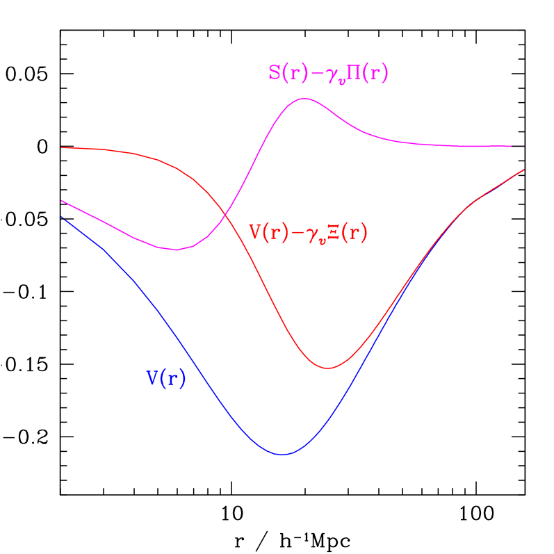
The sign and the strength of the peak pairs flow depend upon the detailed behaviour of the functions and . As seen in Fig. 7 where for illustration, the former is negative at all separations . By contrast, the latter is positive at distances larger than a few smoothing radii but goes negative at smaller scales, regardless of the exact value of . The mean streaming of random field points is also shown in Fig. 7 for comparison. Peak-peak exclusion leads to a deficit of pairs at separation comparable to the filtering scale. It adds to the smoothing and further damps the relative velocity of peaks out to distances that are much larger than the typical extent of density maxima. This is the reason why the correlation is strongly suppressed relative to when . Still, the term proportional to is most strongly negative at distances of the order of the smoothing length and, therefore, could restore significantly the small-scale mean streaming when the threshold height is less than (for which ). At large enough separations however, the mean streaming of peak pairs is unaffected by small-scale exclusion effects and closely tracks the pairwise velocity of ambient field points.
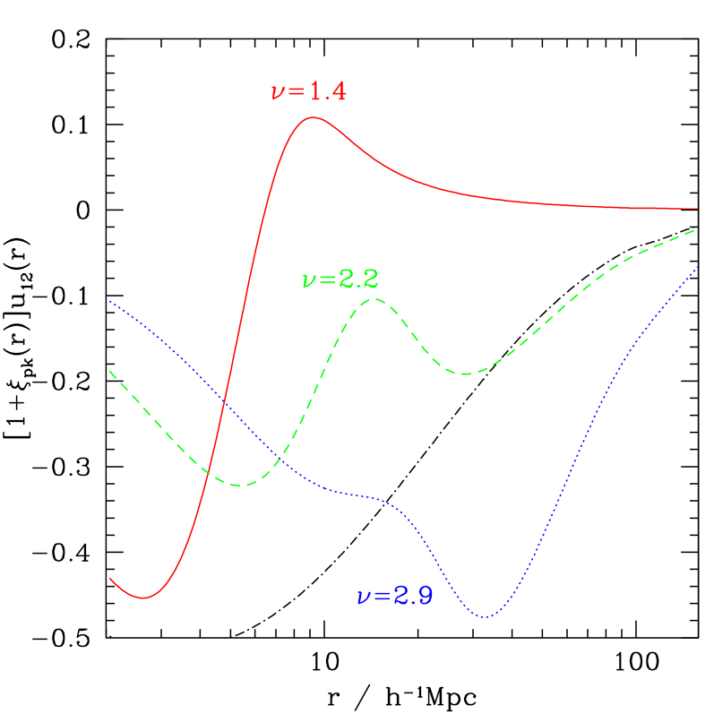
To illustrate the impact of the correlation function on the mean streaming, we show in Fig. 8 the peak pairwise velocity for the smoothing radii , 4 and 6 considered in Sec. IV (recall that the peak height is specified by the relation ). Also shown for comparison is the mean streaming of the (unsmoothed) matter density field (dotted-dashed curve). At the smallest filtering scale for which , the bias parameters are so that is the dominant contribution at all separations. The resulting strong “inward” transport at distances less than a few reflects the fact that these small peaks tend to accrete onto high density regions. At separation , there is a positive net flow presumably owing to the fact that the peaks fall onto nearby distinct overdense regions. Notice that, at all separation, the mean streaming of these maxima is larger than that of the density field, indicating that these small peaks move apart from each other (in an average sense) relative to the matter distribution. At larger filtering scales, the contribution of the first term in the right-hand side of eq.(V.2) increases with the smoothing length as seen from the progressive disappearance of the broad bump at . The maxima identified at () stream towards each other relative to the underlying density field, but their relative motion is strongly suppressed at distances due to the exclusion effect mentioned above.
V.3 Pair conservation equation
So long as peaks do not merge, the time evolution of the peak correlation function is governed by the pair conservation equation. Transforming the time variable to the scale factor, this equation can be written as
| (60) |
where and are the comoving separation and scaled pairwise velocity, respectively. The root-mean-square (rms) variance (computed from eq. 1) defines the length scale for the values of cosmological parameters used here.
Following the approach outlined in Smith et al. (2008), the general solution of eq. (60) can be found by solving the characteristic equation
| (61) |
This equation gives which, upon insertion into the pair conservation equation (60), allows us to write down a first order ordinary differential equation along the characteristics,
| (62) |
where it is understood that Smith et al. (2008).
We will not attempt to solve eq. 62 since, as recognised by Smith et al. (2008); Crocce & Scoccimarro (2008), nonlinearity in the divergence of the pairwise velocity, which is lacking here, is a crucial ingredient in the redshift evolution of the baryon acoustic signature. Instead, we will simply estimate the first order change in the initial separation of peak pairs, , induced by coherent motions across the acoustic scale, . To proceed, we assume that the peaks move according to the Zeldovich ansatz described above, an approximation expected to be valid only in the early (quasi-linear) stages of gravitational clustering. Owing to the near constancy of the peak pairwise velocity at those scales, we can write where . For the maxima considered above, we find , -0.25 and -0.74 with increasing . For comparison, for the dark matter. These values are consistent with those found by Smith et al. (2008). Therefore, at the linear order, changes in the acoustic signature of will be roughly at the percent level. This suggests that some of the enhancement of the BAO in the initial correlation of density maxima may survive in the correlation of high redshift density peaks. Clearly, a thorough numerical investigation and detailed analytic modelling will be needed to ascertain how much of this effect propagates into the late-time clustering of galaxies.
VI Conclusions
We have investigated the strength of the baryon acoustic signature in the 2-point correlation of maxima of the linear (Gaussian) density field . To this purpose, we examined in Sec. III the large-scale asymptotics of the peak correlation and derived the leading order contribution, eq. (44). In contrast to the analysis of BBKS, spatial derivatives of the linear density correlation were included in our derivation. These derivatives are not negligible for generic CDM power spectra, especially around the BAO scale where they exhibit large oscillations. we find that the leading asymptotic behaviour of the peak correlation is governed by three terms : a term previously derived in BBKS plus two terms involving the spatial derivatives and of the linear density correlation. The relative contribution of these functions is controlled by two independent bias parameters, and (The third being , see eq. 45). We also showed that the large-scale asymptotics of can be thought as arising from a nonlinear, local biasing relation, eq. 47, involving second derivatives of the density field.
In Sec. IV, we demonstrated that those extra terms have a large impact on the correlation of density maxima in the vicinity of the BAO. The results are sensitive to the exact value of the threshold height , the smoothing length , the filter shape and the high- tail of the transfer function. For the Gaussian filter adopted throughout this paper, the contrast of the baryon acoustic signature can be significantly enhanced relative to that in the linear matter correlation when the peak height is in the range . This boost originates from the oscillatory behaviour of and around the sound horizon scale. For instance, we find that, at filtering scale , the contrast of the BAO in the correlation of density maxima of height is about twice as large as in . The amplification fades as we go to larger peak height. For a peak height of the order of unity, can exhibit several bumps which reflect those of around the BAO scale. For a threshold height less than , the original acoustic peak is smeared out by the negative contribution of the term .
To avoid the divergence of the (fourth order) spatial derivative of the density correlation, we have filtered the density field with a Gaussian window. The main drawback of this window function is the lack of a well-defined mass and spatial extent associated to the density fluctuations. A top hat filter appears better motivated in the context of, e.g., the spherical infall model, although it does not produce an infinitely differentiable density field for generic CDM power spectra. Furthermore, the differentiability of the density field depends strongly upon the small-scale behaviour of the transfer function. Fluctuations in the matter density are damped on scales smaller than the free-streaming length of the dark matter particle. In the CDM cosmology considered here, the velocity dispersion of the dark matter particle is negligible. By contrast, Warm Dark Matter (WDM) particles such as massive neutrinos for example can suppress the matter power spectrum on galaxy scales Bond et al. (1980). For these reasons, we also discussed in Sec. IV how the BAO changes with the window function and the free-streaming cutoff. We found that the correlation of density maxima is more sensitive to the properties of the dark matter particle(s) than the matter correlation itself. This follows from the dependence of the peak biasing upon the second derivatives of the density field. However, whether the baryon acoustic signature in the clustering of peaks varies significantly with the nature of dark matter remains to be determined.
In Sec. V, we calculated the pairwise velocity of peak pairs at leading order. We showed that it is consistent with the nonlinear local biasing relation inferred from the 2-point correlation of density maxima, provided that the peak velocity field receives a contribution from the gradient of the density field. Explicitly, the leading-order peak correlation and mean streaming can be derived from the nonlinear local biasing relation
| (63) |
where we have dropped some factors for clarity and is the linear matter velocity field. This particular bias relation may be helpful to translate the Lagrangian analysis performed in this paper into quantitative predictions for the baryon oscillation in the low redshift distribution of galaxies, which is currently the primary observable proxy of the baryonic acoustic oscillations. Using the formalism introduced by Fry & Gaztañaga (1993), one may conceive of sophisticated extensions of the halo model halomodel that would include derivatives of the density field, so as to ascertain how much of the amplification of the acoustic signature in the initial clustering of density maxima propagates into the late-time correlation of galaxies and clusters. Extensions which, as a general criterion, reproduce the observed properties of the galaxy distribution, would provide an interesting complement to current local biasing models.
We emphasise that the calculations presented in this paper are performed in the initial conditions. As nonlinearities progress, the late-time acoustic signature is smeared out by structure formation as reported by many authors using N-body simulations baosimu . This might explain why numerical investigations of the clustering of dark matter haloes have not shown thus far any evidence for an amplification of the BAO. Interestingly however, preliminary results from a large suite of N-body simulations hint at a an enhancement of the contrast of the baryonic signature in the clustering of low redshift dark matter haloes resmith . In this regard, it is also worth noticing that the clustering of the SDSS (Sloan Digital Sky Survey) LRG (Luminous Red Galaxies) sample Eisenstein et al. (2005), for instance, shows a slightly sharper acoustic peak than expected from linear theory and smearing due to nonlinearities. However, one should remember that the data points are strongly correlated, so that a very high acoustic peak is actually allowed by the current CDM cosmology. Future redshift surveys such as ADEPT, BOSS, CIP, DES, HETDEX, LSST, Pan-STARRS, PAU, WiggleZ or WFMOS galaxysurveys , which will obtain redshifts for millions of galaxies, should achieve an exquisite precision on the shape of the baryon acoustic signature in the clustering of galaxies. Beyond the nature of dark energy, a precise measurement of the BAO could also place constraints on galaxy biasing and the physical mechanisms that cause it.
Acknowledgements.
I am indebted to Ravi Sheth for pointing out the inconsistency of the expression for the peak mean streaming in an earlier version of this manuscript. I would also like to thank Robert Smith for helpful comments on a preliminary draft; Ilian Iliev and Uros̆ Seljak for interesting discussions; Martin Crocce and Teppei Okumura for stimulating correspondence. This work is supported by the Swiss National Foundation under contract No. 200021-116696/1.Appendix A Mean streaming of peak pairs
A.1 Correlations of velocity field
Let us introduce the scaled velocity field . The rms variance is the three-dimensional proper velocity dispersion of random field points, which is at present time in the cosmology considered here. Also, the notational shorthand will designate the difference . The auto-correlation of the velocity and its cross-correlations with the fields , and can be written as
| (64) | |||||||
Here designates the components of . Notice that and are the radial and transverse correlation functions of the velocity field corrvel . For sake of completeness, the various angle average correlations are
| (65) | |||||
for the Gaussian density field considered here. The functions and satisfy the relation . Like the spectral width , the parameter characterises the range over which the velocity power spectrum is large. It should be noted that the latter peaks on scale much larger than the density power spectrum. Also, the correlation is proportional to the mean streaming of ambient field points,
| (66) |
which is mass weighted by the densities at and .
A.2 Mean streaming at leading order
The calculation of the peak pairwise velocity is more intricate than the peak correlation since we have three additional degrees of freedom, but it closely follows the analysis described in Sec. III.
The line of sight pairwise velocity weighted over all pairs with comoving separation can be expressed as
The local peak density is given by equation (7), supplemented by the appropriate conditions to select those maxima with a certain threshold height. To obtain the average pair velocity as a function of separation , we need to calculate the 2-point probability distribution for the variables . At zero lag, both and are uncorrelated with the density and the Hessian . Hence, the covariance of the components is a block matrix which reads
| (68) |
Similarly, the covariance of the Hessian, and the cross-covariance between and the entries are
| (71) | |||||
| (74) |
Proceeding as in Sec. III, we now consider the regime where all the correlations are much less than unity. The 2-point probability distribution can thus be expanded in the small perturbation ,
| (75) |
Here designates the 1-point probability density. As before, the (now ) matrix denotes the covariances at different comoving positions. It has a (unique) harmonic decomposition in term of the matrices (equation (12). The computation of these matrices is, however, unnecessary as we will see later. Furthermore, the quadratic form now reads
| (76) | |||||
We note that the velocity dispersion of density maxima is lower by a factor than that of random field points Bardeen et al. (1986). One has for a smoothing length . Moreover, eq. (76) leads to a one-point probability distribution separable into the product , where is the one-point distribution of the density and its second derivatives, and is the velocity distribution of peaks,
| (77) |
The separability of the one-point distribution separability considerably simplifies the calculation.
Taking the product mixes the various multipole matrices , so that the result depends on the correlation functions of , , and in a rather complicated way. Averaging over the directions gives
| (78) |
where the block matrices have the same dimensions as . The minus sign in the right-hand side of eq. 78 arises from the negative parity of the correlations and . Owing to the angular average, the calculation of the can be avoided by writing down the entries of using the relations eq. (II.2) and (A.1), and retaining only those components involving odd products of the unit vector . A tedious calculation shows that and can be cast into the form
| (82) | |||||
| (85) |
The functions are
| (86) |
where we have omitted the explicit -dependence of the correlations for brevity. The matrices have the components of the vector as entries,
| (90) | |||||
| (94) | |||||
| (98) |
We have also set
| (99) |
The matrix is identically zero.
The rest of the calculation is easily accomplished owing to the factorisation of the one-point probability distribution . Notice that the scalar contains terms linear and quadratic in and . After integrating out the velocities, the linear terms vanish and we eventually find
Transforming to the set of variables and substituting the expressions (45) of the bias parameters and , the mean streaming of peak pairs can be recast into the form of equation (V.2).
References
- (1) P.J.E. Peebles, J.T. Yu, Astrophys. J. , 162, 815 (1970); R. Sunyaev, Ya.-B Zeldovich, Astrophys. J. Suppl. Ser., 7, 3 (1970); J.R. Bond, G. Efstathiou, Astrophys. J. , 285, L45 (1984); J.A. Holtzmann, Astrophys. J. Suppl. , 71, 1 (1989); W. Hu, N. Sugiyama, Astrophys. J. , 471, 542 (1996); D.J. Eisenstein, W. Hu, Astrophys. J. , 496, 605 (1998).
- Eisenstein et al. (2005) D.J. Eisenstein, et al., Astrophys. J. , 633, 560 (2005).
- (3) S. Cole, et al., Mon. Not. R. Astron. Soc. , 362, 505 (2005); G. Hütsi, Astron. Astrophys. , 449, 891 (2006); M. Tegmark, et al., Phys. Rev. D. , 74, 123507 (2006); W.J. Percival, et al., Astrophys. J. , 657, 51 (2007); W.J. Percival, et al., Mon. Not. R. Astron. Soc. , 381, 1053 (2007); C. Blake, A. Collister, S. Bridle, O. Lahav, Mon. Not. R. Astron. Soc. , 374, 1527 (2007); N. Padmanabhan, et al., Mon. Not. R. Astron. Soc. , 378, 852 (2007); T. Okumura, et al., Astrophys. J. , 676, 889 (2008).
- Estrada et al. (2008) J. Estrada, E. Sefusatti, J.A. Frieman, ArXiv Astrophysics eprint:astro-ph/0801.3485 (2008).
- (5) W. Hu, M. White, Astrophys. J. , 471, 30 (1996); D.J. Eisenstein, W. Hu, M. Tegmark, Astrophys. J. , 504, L57 (1998); A. Cooray, W. Hu, D. Huterer, M. Joffre, Astrophys. J. , 557, L7 (2001); W. Hu, Z. Haiman, Phys. Rev. D. , 68, 063004 (2003); C. Blake, K. Glazebrook, Astrophys. J. , 594, 665 (2003); E.V. Linder, Phys. Rev. D. , 68, 3504 (2003); T. Matsubara, Astrophys. J. , 615, 573 (2004); L. Amendola, C. Quercellini, E. Giallongo, Mon. Not. R. Astron. Soc. , 357, 429 (2005); C. Blake, S. Bridle, Mon. Not. R. Astron. Soc. , 363, 1329 (2005); K. Glazebrook, C. Blake, Astrophys. J. , 631, 1 (2005); D. Dolney, B. Jain, M. Takada, Mon. Not. R. Astron. Soc. , 366, 884 (2006); H. Zhan, L. Knox, Astrophys. J. , 644, 663 (2006); C. Blake, et al., Mon. Not. R. Astron. Soc. , 365, 255 (2006); N. Padmanabhan, M. White, ArXiv Astrophysics eprint:astro-ph/0804.0799 (2008); M. Shoji, D. Jeong, E. Komatsu, ArXiv Astrophysics eprint:astro-ph/0805.4238 (2008).
- (6) Magnification bias and, to a lesser extent, stochastic deflections also affect baryonic features in the 3D galaxy correlation. See, for instance, T. Nishimichi, et al., Pub. Astron. Soc. Jap., 59, 93 (2007); L. Hui, E. Gaztañaga, M. Loverde, Phys. Rev. D. , 76, 103502 (2007); A. Vallinotto, S. Dodelson, C. Schimd, J.-P. Uzan, Phys. Rev. D. , 75, 103509 (2007); M. Loverde, L. Hui, E. Gaztañaga, Phys. Rev. D. , 77, 023512 (2008); L. Hui, E. Gaztañaga, M. Loverde, Phys. Rev. D. , 77, 063526 (2008).
- (7) H-J. Seo, D.J. Eisenstein, Astrophys. J. , 598, 720 (2003); M. White, Astro-particle Phys. , 24, 334 (2005); V. Springel, et al., Nature (London) , 435, 629 (2005); R.E. Angulo, et al., Mon. Not. R. Astron. Soc. , 362, L25 (2005). E. Huff, A.E. Schultz, M. White, D.J. Schlegel, M.S. Warren, Astro-particle Phys. , 26, 351 (2007); Z. Ma, Astrophys. J. , 665, 887 (2007); R.E. Angulo, C.M. Baugh, C.S. Frenk, C.G. Lacey, Mon. Not. R. Astron. Soc. , 383, 755 (2008); R. Takahashi, et al., ArXiv Astrophysics eprint:astro-ph/0802.1808 (2008); A.G. Sanchez, C.M. Baugh, R. Angulo, ArXiv Astrophysics eprint:astro-ph/0804.0233 (2008).
- Meiksin et al. (1999) A. Meiksin, M. White, J.A. Peacock, Mon. Not. R. Astron. Soc. , 304, 851 (1999).
- Seo & Eisenstein (2005) H.J.-Seo, D.J. Eisenstein, Astrophys. J. , 633, 575 (2005).
- Jeong & Komatsu (2006) D. Jeong, E. Komatsu, Astrophys. J. , 651, 619 (2006).
- Schultz & White (2006) A.E. Schultz, M. White, Astro-particle Phys. , 25, 172 (2006).
- Guzik et al. (2007) J. Guzik, G. Bernstein, R.E. Smith, Mon. Not. R. Astron. Soc. , 375, 1329 (2007).
- Eisenstein et al. (2007) D.J. Eisenstein, H.-J. Seo, M. White, Astrophys. J. , 664, 660 (2007).
- Smith et al. (2007) R.E. Smith, R. Soccimarro, R.K. Sheth, Phys. Rev. D. , 75, 063512 (2007).
- Matarrese & Pietroni (2007) S. Matarrese, M. Pietroni, JCAP, 06, 026 (2007).
- Crocce & Scoccimarro (2008) M. Crocce, R.Scoccimarro, Phys. Rev. D. , 77, 023533 (2008).
- Smith et al. (2008) R.E. Smith, R.Scoccimarro, R.K. Sheth, Phys. Rev. D. , 77, 043525 (2008).
- Matsubara (2008) T. Matsubara, Phys. Rev. D. , 77, 063530 (2008).
- Matarrese & Pietroni (2008) S. Matarrese, M. Pietroni, Mod. Phys. Lett. A, 23, 25 (2008).
- Seo et al. (2008) H.-J. Seo, E.R. Siegel, D.J. Eisenstein, M. White, ArXiv Astrophysics eprint:astro-ph/0805.0117 (2008).
- (21) D. Jeong, E. Komatsu, ArXiv Astrophysics eprint:astro-ph/0805.2632
- Eisenstein et al. (2007) D.J. Eisenstein, H.-J. Seo, E. Sirko, D.N. Spergel, Astrophys. J. , 664, 675 (2007).
- Coles (1993) P. Coles, Mon. Not. R. Astron. Soc. , 262, 1065 (1993).
- Scherrer & Weinberg (1998) R.J. Scherrer, D.H. Weinberg, Astrophys. J. , 504, 607 (1998).
- Fry & Gaztañaga (1993) J.N. Fry, E. Gaztañaga, Astrophys. J. , 413, 447 (1993).
- Szalay (1988) A.S. Szalay, Astrophys. J. , 1988, 333, 21.
- (27) Komatsu, et al., Astrophys. J. Suppl. , 148, 119 (2003); P. Creminelli, N. Alberto, L. Senatore, M. Tegmark, M. Zaldarriaga, JCAP, 06, 004 (2006); A. Yadav, B.D. Wandelt, ArXiv Astrophysics eprint:astro-ph/0712.1148 (2007); A. Slosar, et al., ArXiv Astrophysics eprint:astro-ph/0805.3580 (2008).
- (28) E. Komatsu, et al., ArXiv Astrophysics eprint:astro-ph/0803.0547 (2008); E.L. Wright, et al., ArXiv Astrophysics eprint:astro-ph/0803.0577 (2008); J. Dunkley, et al., ArXiv Astrophysics eprint:astro-ph/0803.0586 (2008); M.R. Nolta, et al., ArXiv Astrophysics eprint:astro-ph/0803.0593 (2008); B. Gold, et al., ArXiv Astrophysics eprint:astro-ph/0803.0715 (2008); G. Hinshaw, et al., ArXiv Astrophysics eprint:astro-ph/0803.0732 (2008).
- Bardeen et al. (1986) J.M. Bardeen, J.R. Bond, N. Kaiser, A.S. Szalay, Astrophys. J. , 304, 15 (1986).
- Kaiser (1984) N. Kaiser, Astrophys. J. , 284, L9 (1984).
- Politzer & Wise (1984) D. Politzer, M. Wise, Astrophys. J. , 285, L1 (1984).
- Jensen & Szalay (1986) L.G. Jensen, A.S. Szalay, Astrophys. J. , 305, L5 (1986).
- Doroshkevich (1970) A.G. Doroshkevich, Astrofizika, 3, 175 (1970).
- Hoffman & Shaham (1985) Y. Hoffman, J. Shaham, Astrophys. J. , 297, 16 (1985).
- Peacock & Heavens (1985) J.A. Peacock, A.F. Heavens, Mon. Not. R. Astron. Soc. , 217, 805 (1985).
- Coles (1989) P. Coles, Mon. Not. R. Astron. Soc. , 238, 319 (1989).
- Lumsden, Heavens & Peacock (1989) S.L. Lumsden, A.F. Heavens, J.A. Peacock, Mon. Not. R. Astron. Soc. , 238, 293 (1989).
- Kaiser & Davis (1985) N. Kaiser, M. Davis, Astrophys. J. , 297, 365 (1985).
- Otto et al. (1986) S. Otto, H.D. Politzer, M.B. Wise, Phys. Rev. Lett. , 56, 2772 (1986).
- Cen (1998) R. Cen, Astrophys. J. , 509, 494 (1998).
- Desjacques (2007) V. Desjacques, Mon. Not. R. Astron. Soc. , 388, 638 (2008).
- Desjacques & Smith (2008) V. Desjacques, R.E. Smith, Phys. Rev. D. , 78, 023527 (2008).
- Adler & Taylor (2007) R.J. Adler, J. Taylor, Random Fields and Geometry, Springer Monographs in Mathematics, Springer, New York (2007).
- (44) U. Seljak, M. Zaldarriaga, Astrophys. J. , 469, 437 (1996); A. Lewis, A. Challinor, A. Lasenby, Astrophys. J. , 538, L473 (2000);
- (45) W. Hu, N. Sugiyama, Astrophys. J. , 471, 542 (1996); K. Yamamoto, N. Sugiyama, H. Sato, Phys. Rev. D. , 56, 7566 (1997); K. Yamamoto, N. Sugiyama, H. Sato, Astrophys. J. , 501, 442 (1998); S. Naoz, R. Barkana, Mon. Not. R. Astron. Soc. , 362, 1047 (2005).
- Kac (1943) M. Kac, Bull. Am. Math. Soc., 49, 314 (1943).
- Rice (1954) S.O. Rice, Mathematical analysis of random noise, in Selected Papers on Noise and Stochastic Processes, Dover, New York (1954).
- Belyaev (1967) J.K. Belyaev, Sov. Math. Dokl., 8, 1107 (1967).
- Cline et al. (1987) J.M. Cline, H.D. Politzer, S.-Y. Rey, M.B. Wise, Commun. Math. Phys., 112, 217 (1987).
- Bond et al. (1991) J.R. Bond, S. Cole, G. Efstathiou, N. Kaiser, Astrophys. J. , 379, 440 (1991).
- Press & Schechter (1974) W.H. Press, P. Schechter, Astrophys. J. , 187, 425 (1974).
- Gunn & Gott (1972) J.E. Gunn, J.R. Gott III, Astrophys. J. , 176, 1 (1972).
- Mo & White (1996) H.J. Mo, S.D.M. White, Mon. Not. R. Astron. Soc. , 282, 347 (1996).
- Sheth & Tormen (1999) R.K Sheth, G. Tormen, Mon. Not. R. Astron. Soc. , 308, 119 (1999).
- Cole & Kaiser (1989) S. Cole, N. Kaiser, Mon. Not. R. Astron. Soc. , 237, 1127 (1989).
- Sheth & Tormen (2002) R.K. Sheth, G. Tormen, Mon. Not. R. Astron. Soc. , 329, 61 (2002).
- Kauffmann et al. (1999) G. Kauffmann, J.M. Colberg, A. Diafero, S.D.M. White, Mon. Not. R. Astron. Soc. , 303, 188 (1999).
- (58) D. Reed, et al., Mon. Not. R. Astron. Soc. , 346, 565 (2003); K. Heitmann, Z. Lukić, S. Habib, P.M. Ricker, Astrophys. J. , 646, L1 (2006); I.T. Iliev, et al., Mon. Not. R. Astron. Soc. , 369, 1625 (2006); D. Reed, R. Bower, C.S. Frenk, A. Jenkins, T. Theuns, Mon. Not. R. Astron. Soc. , 374, 2 (2007); Z. Lukić, K. Heitmann, S. Habib, S. Bashinsky, P.M. Ricker, Astrophys. J. , 671, 1160 (2007); O. Zahn, et al., Astrophys. J. , 654, 12 (2007).
- Bond et al. (1980) J.R. Bond, G. Efstathiou, J. Silk, Phys. Rev. Lett. , 45, 1980 (1980).
- (60) P. Bode, J.P. Ostriker, N. Turok, Astrophys. J. , 556, 93 (2001); S.H. Hansen, J. Lesgourgues, S. Pastor, J. Silk, Mon. Not. R. Astron. Soc. , 333, 544 (2002).
- Dalal et al. (2008) N. Dalal, M. White, J.R. Bond, A. Shirokov, ArXiv Astrophysics eprint:astro-ph/0803.3453 (2008).
- Zeldovich (1970) Y.B. Zeldovich, Astron. Astrophys. , 5, 84 (1970).
- Peebles (1980) P.J.E Peebles, The Large-Scale Structure of the Universe (Princeton University Press, 1980).
- Grinstein & Wise (1987) B. Grinstein, M.B. Wise, Astrophys. J. , 320, 448 (1987).
- (65) R.G. Mann, A.F. Heavens, J.A. Peacock, Mon. Not. R. Astron. Soc. , 263, 798 (1993); S. Borgani, P. Coles, L. Moscardini, Mon. Not. R. Astron. Soc. , 271, 223 (1994).
- (66) J.R. Bond, S.T. Myers, Astrophys. J. Suppl. , 103, 1 (1996); J.R. Bond, S.T. Myers, Astrophys. J. Suppl. , 103, 41 (1996); J.R. Bond, S.T. Myers, Astrophys. J. Suppl. , 103, 63 (1996).
- Peebles (1976) P.J.E. Peebles, Astrophys. Space Science , 45, 3 (1976).
- Davis & Peebles (1977) M. Davis, P.J.E. Peebles, Astrophys. J. Suppl. , 34, 425 (1977).
- Sheth et al. (2001) R.K. Sheth, A. Diafero, L. Hui, R. Scoccimarro, Mon. Not. R. Astron. Soc. , 326, 463 (2001).
- (70) A.J. Benson, S. Cole, C.S. Frenk, C. Baugh, C. Lacey, Mon. Not. R. Astron. Soc. , 311, 793 (2000); J.A. Peacock, R.E. Smith, Mon. Not. R. Astron. Soc. , 318, 1144 (2000); U. Seljak, Mon. Not. R. Astron. Soc. , 318, 203 (2000); R. Scoccimarro, R.K. Sheth, L. Hui, B. Jain, Astrophys. J. , 546, 20 (2001); A. Berlind, D. Weinberg, Astrophys. J. , 575, 587 (2002).
- (71) C.S. Frenk, S.D.M. White, M. Davis, G. Efstathiou, Astrophys. J. , 327, 507 (1988); N. Katz, T. Quinn, J.M. Gelb, Mon. Not. R. Astron. Soc. , 265, 689 (1993); C. Porciani, A. Dekel, Y. Hoffman, MNRAS, 332, 325 (2002).
- (72) Robert Smith, private communication.
- (73) ADEPT: http://www.jhu.edu/news_info/news/home06/ aug06/adept.html; BOSS: http://www.sdss3.org/cosmology.php; CIP: http://cfa-www.harvard.edu/cip; DES: http://www.darkenergysurvey.org; HETDEX: http://www.as.utexas.edu/hetdex; LSST: H. Zhan, L. Knox, T.J. Anthony, V. Margoniner, Astrophys. J. , 640, 8 (2006) (http://www.lsst.org); Pan-STARRS: http://pan-starrs.ifa.hawaii.edu; PAU: N. Benitez et al., ArXiv Astrophysics eprint :astro-ph/0807.0535; WiggleZ: http://astronomy.swin.edu.au; WFMOS : Glazebrook et al., ArXiv Astrophysics eprint : astro-ph/0507457 (2005).
- (74) A.S. Monin, A.M. Yaglom, Statistical Fluid Mechanics (Cambridge MIT Press, 1975); K. Górski, Astrophys. J. , 332, L7 (1988).