Loebl–Komlós–Sós Conjecture: dense case

Abstract

We prove a version of the Loebl–Komlós–Sós Conjecture for dense graphs. For each $q>0$ there exists a number $n_{0}\in\mathbb{N}$ such that for each $n>n_{0}$ and $k>qn$ the following holds: if $G$ is a graph of order $n$ with at least $\tfrac{n}{2}$ vertices of degree at least $k$, then each tree of order $k+1$ is a subgraph of $G$.

Keywords: Loebl–Komlós–Sós Conjecture, Ramsey number of trees.

1 Introduction

Embedding problems play a central role in Graph Theory. A variety of graph embeddings (subgraphs, minors, subdivisions, immersions, etc) have been studied extensively. A graph (finite, undirected, loopless, simple; here as well as in the rest of the paper) $H$ embeds in a graph $G$ if there exists an injective mapping $\phi:V(H)\rightarrow V(G)$ which preserves the edges of $H$, i. e., $\phi(x)\phi(y)\in E(G)$ for every edge $xy\in E(H)$. As a synonym we say that $G$ contains $H$ (as a subgraph) and write $H\subseteq G$. Let $\mathcal{H}$ be a family of graphs. The graph $G$ is $\mathcal{H}$-universal if it contains every graph from $\mathcal{H}$. This fact is denoted by $\mathcal{H}\subseteq G$.

In this paper we investigate embeddings of trees. This topic has received considerable attention during the last 40 years. The class $\mathcal{T}_{\ell}$ consists of all trees of order $\ell$. One can ask which properties force a graph $G$ to be $\mathcal{T}_{\ell}$-universal. One sufficient condition for $\mathcal{T}_{\ell}$-universality can be given in terms of minimum degree.

Fact 1.1.

If a graph $G$ has the minimum degree $\delta(G)\geq k$ then $\mathcal{T}_{k+1}\subseteq G$.

To prove Fact 1.1 it suffices to embed a given tree $T\in\mathcal{T}_{k+1}$ greedily in the host graph $G$. Loebl, Komlós and Sós conjectured (see [10]) that the minimum degree condition can be relaxed to a median degree one.

Conjecture 1.2 (LKS Conjecture).

Let $G$ be a graph of order $n$. If at least $\tfrac{n}{2}$ of the vertices of $G$ have degree at least $k$, then $\mathcal{T}_{k+1}\subseteq G$.

The bound on $k$ of the minimal degree of large degree vertices cannot be decreased. Indeed, if $G$ is a graph with maximum degree $k-1$, then it does not contain a star $K_{1,k}$. The graph shown in Figure 1 shows that the requirement on the number of large degree vertices cannot be relaxed substantially below $\frac{n}{2}$.

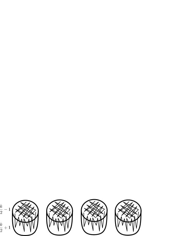
Figure 1: A graph with almost half of its vertices of degree $k$ which does not contain a path of length $k$.

See [28] and [13] for further discussions.

There have been several partial results concerning the LKS Conjecture. In [3], Bazgan, Li and Woźniak proved the conjecture for paths. Piguet and Stein [22] proved that the LKS Conjecture is true when restricted to the class of trees of diameter at most 5, improving upon results of Barr and Johansson [2] and of Sun [26]. There are several results proving the LKS Conjecture under additional assumptions on the host graph. Soffer [25] showed that the conjecture is true if the host graph has girth at least 7. Dobson [7] proved the conjecture when the complement of the host graph does not contain a $K_{2,3}$.

A special case of the LKS Conjecture is when $k=\tfrac{n}{2}$. This is often referred to as the ($\tfrac{n}{2}$–$\tfrac{n}{2}$–$\tfrac{n}{2}$) Conjecture, or Loebl’s Conjecture. Zhao [28] proved the conjecture for large graphs.

Theorem 1.3.

There exists a number $n_{0}\in\mathbb{N}$ such that if a graph $G$ of order $n>n_{0}$ has at least $\tfrac{n}{2}$ of the vertices of degrees at least $\tfrac{n}{2}$, then $\mathcal{T}_{\lfloor\tfrac{n}{2}\rfloor+1}\subseteq G$.

An approximate version of the LKS Conjecture for dense graphs was proven by Piguet and Stein [23].

Theorem 1.4.

For each $q,\varepsilon>0$ there exists a number $n_{0}$ such that for each $n>n_{0}$ and $k>qn$ the following holds. If $G$ is a graph of order $n$ with at least $\tfrac{n}{2}$ vertices of degree at least $(1+\varepsilon)k$, then $\mathcal{T}_{k+1}\subseteq G$.

In this paper we strengthen Theorem 1.4 by removing the $\varepsilon$ term.

Theorem 1.5 (Main Theorem).

For each $q>0$ there exists a number $n_{0}=n_{0}(q)\in\mathbb{N}$ such that for each $n>n_{0}$ and $k>qn$ the following holds. If $G$ is a graph of order $n$ with at least $\tfrac{n}{2}$ vertices of degree at least $k$, then $\mathcal{T}_{k+1}\subseteq G$.

We can see from our proof of Theorem 1.5 that the requirement on the number of vertices of large degree can be relaxed in the case when $\tfrac{n}{k}$ is far from being an integer.

Theorem 1.6.

For each $q_{2}>q_{1}>0$ such that the interval $[\tfrac{1}{q_{2}},\tfrac{1}{q_{1}}]$ does not contain any integer, there exist $\varepsilon=\varepsilon(q_{1},q_{2})>0$ and $n_{0}$ such that for each $n>n_{0}$ and $k\in(q_{1}n,q_{2}n)$ the following holds: if $G$ is a graph of order $n$ with at least $(\tfrac{1}{2}-\varepsilon)n$ vertices of degree at least $k$, then $\mathcal{T}_{k+1}\subseteq G$.

In the paper, we explicitly prove only Theorem 1.5. In Section 2 we sketch how the proof method can be revised to give Theorem 1.6. However, determining the optimal value of $\varepsilon(q_{1},q_{2})$ remains open. Note also that Theorem 1.5 has slightly weaker assumptions on $G$ than Theorem 1.3 when reduced to the case $k=\lfloor\tfrac{n}{2}\rfloor$ — when $n$ is odd, the requirement on degrees of large vertices in Theorem 1.5 is smaller by one compared to Theorem 1.3.

The property which is considered in the LKS conjecture is given in terms of the median degree. If we consider the average degree instead we obtain a famous conjecture of Erdős and Sós which dates back to 1963.

Conjecture 1.7 (ES Conjecture, [8, p.30]).

Let $G$ be a graph of order $n$ with more than $\tfrac{1}{2}(k-2)n$ edges. Then $\mathcal{T}_{k}\subseteq G$.

If true, the ES Conjecture is sharp. After several partial results on the problem, a breakthrough was achieved by Ajtai, Komlós, Simonovits and Szemerédi, who announced a proof of the Erdős–Sós Conjecture for large $k$.

Theorem 1.8.

There exists a number $k_{0}$ such that for each $k>k_{0}$ the following holds: if a graph $G$ of order $n$ has more than $\tfrac{1}{2}(k-2)n$ edges, then $\mathcal{T}_{k}\subseteq G$.

A version of Theorem 1.8 for $k$ linear in $n$ could be obtained by an application of the Regularity Lemma; such a theorem would be a counterpart to Theorem 1.5. The proof of Theorem 1.8 by Ajtai et al. uses a decomposition technique which substantially generalizes the Regularity Lemma, and which is applicable even to sparse graphs. Hladký, Komlós, Piguet, Simonovits, Stein, and Szemerédi [14, 15, 16, 17] used this decomposition technique to prove an approximate version of the LKS Conjecture (see also [18] for a high-level overview of the proof).

Theorem 1.9.

For each $\varepsilon>0$ there exists a number $k_{0}$ such that for each $k>k_{0}$ the following holds. If $G$ is a graph of order $n$ with at least $(\tfrac{1}{2}+\varepsilon)n$ vertices of degrees at least $(1+\varepsilon)k$, then $\mathcal{T}_{k+1}\subseteq G$.

We believe that the techniques developed for Theorem 1.5 and for Theorem 1.9 can be utilized to proving the LKS Conjecture for $k$ sufficiently large.

The current work builds on techniques of Zhao [28] and of Piguet and Stein [23]. We postpone a detailed discussion of similarities between our approach and theirs and of our own contribution until Section 2. After the first version of this manuscript was posted on the arXiv, Oliver Cooley [5] published an independent proof of Theorem 1.5.

1.1 Ramsey number of trees

In this section we show the connection between the LKS Conjecture and the Ramsey number of trees. For two graphs $F$ and $H$ we write $R(F,H)$ for the Ramsey number of the graphs $F$ and $H$. This is the smallest number $m$ such that in each red/blue edge-coloring of $K_{m}$ there is a red copy of $F$ or a blue copy of $H$. For two families of graphs $\mathcal{F}$ and $\mathcal{H}$ the Ramsey number $R(\mathcal{F},\mathcal{H})$ is the smallest number $m$ such that in each red/blue edge-coloring of $K_{m}$ the graph induced by the red edges is $\mathcal{F}$-universal, or the graph induced by the blue edges is $\mathcal{H}$-universal. Theorem 1.5 implies an almost tight upper bound (up to an additive error of one) on the Ramsey number of pairs of families of trees of similar orders. This partially answers a question of Erdős, Füredi, Loebl and Sós [10]. For a fixed real $p\in(0,\tfrac{1}{2})$ consider two natural numbers $\ell_{1}$ and $\ell_{2}$ such that

$$n_{0}<\ell_{1}\leq\ell_{2}<\tfrac{\ell_{1}}{p}\;,$$ (1.1)

where $n_{0}=n_{0}(\tfrac{p}{2})$ comes from Theorem 1.5. Consider any red/blue edge-coloring of the graph $K_{\ell_{1}+\ell_{2}}$. We color a vertex $v\in V(K_{\ell_{1}+\ell_{2}})$ red if it incident with at least $\ell_{1}$ red edges, and blue otherwise (in which case it is incident with at least $\ell_{2}$ blue edges). Thus at least half of the vertices of $K_{\ell_{1}+\ell_{2}}$ have the same color. Applying Theorem 1.5 to the graph whose edges are induced by this color, we conclude that $R(\mathcal{T}_{\ell_{1}+1},\mathcal{T}_{\ell_{2}+1})\leq\ell_{1}+\ell_{2}$.

For the lower bound, first consider the case when at least one of $\ell_{1}$ and $\ell_{2}$ is odd. It is a well-known fact that there exists a red/blue edge-coloring of $K_{\ell_{1}+\ell_{2}-1}$ such that the red degree of every vertex is $\ell_{1}-1$. Neither a red copy of $K_{1,\ell_{1}}$ nor a blue copy of $K_{1,\ell_{2}}$ is contained in $K_{\ell_{1}+\ell_{2}-1}$ with this coloring. Thus $R(\mathcal{T}_{\ell_{1}+1},\mathcal{T}_{\ell_{2}+1})>\ell_{1}+\ell_{2}-1$. A construction in a similar spirit shows that $R(\mathcal{T}_{\ell_{1}+1},\mathcal{T}_{\ell_{2}+1})>\ell_{1}+\ell_{2}-2$, if both $\ell_{1}$ and $\ell_{2}$ are even. Under the assumptions given by (1.1) we thus have

$$R(\mathcal{T}_{\ell_{1}+1},\mathcal{T}_{\ell_{2}+1}) =\ell_{1}+\ell_{2}\;,\quad\mbox{if $\ell_{1}$ is odd or $\ell_{2}$ is odd, and}$$ (1.2)

$$\ell_{1}+\ell_{2}-1\leq R(\mathcal{T}_{\ell_{1}+1},\mathcal{T}_{\ell_{2}+1}) \leq\ell_{1}+\ell_{2}\;,\quad\mbox{ otherwise.}$$ (1.3)

The ES Conjecture, if true, shows that the lower bound in (1.3) is attained.

Ramsey numbers of several other classes of trees have been investigated; the reader is referred to a survey of Burr [4] and to newer results in [9, 11, 12].

2 Outline of the proof

We iterate the following procedure in steps $i=1,2,3,\ldots$. At the beginning of step $i$ we are given sets $V_{1},\ldots,V_{i-1}$ that were obtained in previous steps. We then find a set $Q\subseteq V(G)\setminus\bigcup_{j<i}V_{j}$ such that at least about a half of the vertices in $Q$ are large (i. e., of degree at least $k$). Furthermore, the set $Q$ is almost isolated from the rest of the graph. Using the Regularity Lemma, we try to embed $T$ in $Q$. If we do not succeed, then we can extract from $Q$ a subset $V_{i}\subseteq Q$ of size approximately $k$ which is nearly isolated from the rest of the graph, and for which at least half of the vertices are large. If we cannot embed $T$ in any of the iterating steps (i. e., $V(G)\setminus\bigcup_{i}V_{i}\cong\emptyset$), we obtain a particular configuration of the graph $G$, called the Extremal Configuration. The structure of $G$ is then very similar to that depicted in Figure 1. In this case, we prove that $T\subseteq G$, without the use of the Regularity Lemma.

In the remainder of the overview, we explain in more detail the proof of the part using the Regularity Lemma, as well as the part when $G$ is in the Extremal configuration.

The Regularity Lemma Part.

Before applying the Regularity Lemma, we first resolve two simple cases. The first one is when $Q$ is close to a bipartite graph with one of its color classes being the large vertices (see Lemma 5.1). The second case (see Lemma 5.5) is when the tree $T$ is locally unbalanced (see the definition on page 5.4). In both cases easy arguments show that $T\subseteq G$.

In other cases we use the Regularity Lemma on the graph $G$ and obtain a cluster graph $\mathbf{G}$. We apply a matching lemma (Lemma 5.8) to the subgraph induced by the clusters in $Q$. This lemma guarantees the existence of one of two certain matching structures in $\mathbf{G}$. Each of these structures exposes a matching $M$ in the cluster graph, and two clusters $A$ and $B$ that are adjacent in $\mathbf{G}$ and that have high average degree to the matching $M$. These structures are called Case I and Case II. The principle of the embedding is to use the edges of $M$ to embed parts of the tree $T$ in them, and use the clusters $A$ and $B$ to connect these parts.

The Extremal Case Configuration.

In the Extremal case we are given disjoint sets $V_{1},\ldots,V_{i}\subseteq V(G)$ such that each of them has size approximately $k$, contains at least nearly $\tfrac{k}{2}$ large vertices, and each set $V_{j}$ is almost isolated from the rest of the graph.

If the sets $V_{1},\ldots,V_{i}$ exhaust the whole graph $G$, we are able to show $T\subseteq G$ as follows. We find a set $V_{i_{0}}$ so that most of $T$ can be embedded in $V_{i_{0}}$. We may need to use a few edges that connect distinct sets $V_{j}$ and embed some part of $T$ outside $V_{i_{0}}$. The way of finding these “bridges” depends on the structure of the tree $T$.

If $V_{1},\ldots,V_{i}$ do not exhaust $G$, the method remains the same. However, it has two possible outcomes. Either we show that $T\subseteq G$ or we are able to exhibit a set $Q\subseteq V\setminus\bigcup_{j<i}V_{j}$ with the properties as above allowing the next step of the iteration.

Strengthening of Theorem 1.5 — Theorem 1.6.

The only place where we use the exact bound on the number of large vertices is the last step of the Extremal case. That is, the whole vertex set $V(G)$ is decomposed into sets $V_{1},\ldots,V_{s}$, each of size approximately $k$. Assume now that $k\in(q_{1}n,q_{2}n)$. We have $n=|V_{1}|+|V_{2}|+\ldots+|V_{s}|\approx ks\in(q_{1}sn,q_{2}sn)$, yielding that the the interval $(q_{1}s,q_{2}s)$ must contain 1 (or at least to be “close to 1”). Thus the Extremal case cannot occur when $[\tfrac{1}{q_{2}},\tfrac{1}{q_{1}}]\cap\mathbb{N}=\emptyset$. This suffices to prove Theorem 1.6.

Relation to previous work.

The proof of Theorem 1.5 is inspired by techniques used to prove Theorem 1.4 ([23]) and Theorem 1.3 ([28]). Both these papers build on a seminal paper of Ajtai, Komlós and Szemerédi [1] where an approximate version of the $(\tfrac{n}{2}$–$\tfrac{n}{2}$–$\tfrac{n}{2})$ Conjecture was proven. In [1] the basic strategy is outlined. It is worth noting that even though [1] addresses explicitly only the $(\tfrac{n}{2}$–$\tfrac{n}{2}$–$\tfrac{n}{2})$ Conjecture the proof actually yields Theorem 1.4 in the regime $\tfrac{k}{n}\geq\tfrac{1}{2}$. As in the proof overview above, the key step is a certain matching lemma applied to the cluster graph of the host graph.

The key ingredient in [28] was to identify — using the approach of Ajtai, Komlós and Szemerédi combined with the Stability method of Simonovits [24] — one extremal case. This extremal case was analysed and resolved by ad-hoc methods. The main contribution of [23] is a more general matching lemma, which is applicable even when $\tfrac{k}{n}<\tfrac{1}{2}$. In this paper we further strengthen the matching lemma from [23]. The Extremal case is an extensive generalization of the Extremal case from [28].

Algorithmic questions.

Let us remark that our proof of Theorem 1.5 yields a polynomial time algorithm for finding an embedding of each tree $T\in\mathcal{T}_{k+1}$ in $G$, given that $k$ and $G$ satisfy the conditions of Theorem 1.5. Indeed, all the existential results we use (Regularity Lemma, and various matching theorems) are known to have polynomial-time constructive algorithmic counterparts. We omit details.

3 Notation and preliminaries

For $n\in\mathbb{N}$ we write $[n]=\{1,2,\ldots,n\}$. The symbol $\triangle$ means the symmetric difference of two sets. The function $\mathrm{ci}:\mathbb{R}\rightarrow\mathbb{Z}$ is the closest integer function defined by $\mathrm{ci}(x)=\lfloor x\rfloor$ if $x-\lfloor x\rfloor<0.5$, and $\mathrm{ci}(x)=\lceil x\rceil$ otherwise.

We use standard graph theory terminology and notation, following Diestel’s book [6]. We define here only symbols that are not used there. The order of a graph $H$ and the number of its edges are denoted by $v(H)$ and $e(H)$, respectively. For two vertex sets $X$ and $Y$ we write $E(X,Y)$ for the set of edges with one end-vertex in $X$ and the other in $Y$. We write $e(X,Y)=|E(X,Y)|$ (note that edges inside $X\cap Y$ get counted only once). When $X$ and $Y$ are disjoint, we write $H[X,Y]$ for the bipartite graph they induced. For a vertex $x$ and a vertex set $X$ we define $\deg(x,X)=\deg_{X}(x)=e(\{x\},X)$. For two sets $X,Y\subseteq V(H)$ we define the average degree from $X$ to $Y$ by $\mathrm{d\overline{eg}}_{H}(X,Y)=\tfrac{e(X,Y\setminus X)}{|X|}$. We write $\mathrm{d\overline{eg}}_{H}(X)$ as a short for $\mathrm{d\overline{eg}}_{H}(X,V(H))$. Let $X$ and $Y$ are arbitrary (not necessarily disjoint vertex sets). We define two variants of the minimum degree: $\delta(X)=\min_{v\in X}\deg(v)$, and $\delta(X,Y)=\min_{v\in X}\deg(v,Y)$. In this case, we may write $H$ in the subscript (e.g. $\delta_{H}(X)$) to emphasize which graph we are dealing with. We denote by $\mathrm{N}(x)$ the set of neighbors of the vertex $x$, by $\mathrm{N}_{X}(x)$ the neighborhood of $x$ restricted to a set $X$, i. e., $\mathrm{N}_{X}(x)=\mathrm{N}(x)\cap X$, and by $\mathrm{N}(X)$ the set of all vertices in $H$ which are adjacent to at least one vertex from $X$, i. e., $\mathrm{N}(X)=\bigcup_{v\in X}\mathrm{N}(v)$.

Let $P=v_{1}v_{2}\ldots v_{\ell}$ be a path. For arbitrary sets of vertices $X_{1},X_{2},\ldots,X_{\ell}$ we say that $P$ is an $X_{1}-X_{2}-\ldots-X_{\ell}$-path if $v_{i}\in X_{i}$ for every $i\in[\ell]$. An edge $xy$ is an $X-Y$ edge if $x\in X$ and $y\in Y$ and a matching $M$ is an $X-Y$ matching if its every edge is an $X-Y$ edge.

A pair $(H,\omega)$ is a weighted graph if $H$ is a graph and $\omega:E(H)\rightarrow(0,+\infty)$ is a weight function. For two sets $X,Y\subseteq V(H)$ the weight of the edges crossing from $X$ to $Y$ is defined by $\omega(X,Y)=\sum_{xy\in E(X,Y)}\omega(xy)$. Denote also by $\omega$ the weighted degree, $\omega(v)=\sum_{u\in V(H),vu\in E(H)}\omega(vu)$. For a vertex $v$ and a vertex set $X$ we define $\omega(v,X)$ analogously to $\deg(v,X)$.

We omit rounding symbols when this does not effect the correctness of calculations.

3.1 Trees

Let $T$ be a rooted tree with a root $r\in V(T)$. We define a partial order $\preceq$ on $V(T)$ by saying that $a\preceq b$ if and only if the vertex $b$ lies on the (unique) path connecting $a$ with $r$. If $a\preceq b$ and $a\neq b$ we say that $a$ is below $b$. A vertex $a$ is a child of $b$ if $a\preceq b$ and $ab\in E(T)$. The vertex $b$ is then the parent of $a$. $\mathrm{Ch}(b)$ denotes the set of children of $b$. The parent of a vertex $a$ is denoted $\mathrm{Par}(a)$ (note that $\mathrm{Par}(a)$ is undefined if $a=r$). We extend the definitions of $\mathrm{Ch}(\cdot)$ and $\mathrm{Par}(\cdot)$ to an arbitrary set $U\subseteq V(T)$ by $\mathrm{Par}(U)=\bigcup_{u\in U}\mathrm{Par}(u)$ and $\mathrm{Ch}(U)=\bigcup_{u\in U}\mathrm{Ch}(u)$. We say that a tree $T_{1}\subseteq T$ is induced by a vertex $x\in V(T)$ if $V(T_{1})=\{v\in V(T)\>:\>v\preceq x\}$ and we write $T_{1}=T(r,\downarrow x)$, or if the root is obvious from the context $T_{1}=T(\downarrow x)$. Subtrees induced by a vertex are called end subtrees. Other subtrees are called internal subtrees. A subtree $T_{0}$ of $T$ is a full-subtree, if there exists a vertex $y\in V(T)$ and a set $C\subseteq\mathrm{Ch}(y)$, $C\not=\emptyset$ such that $T_{0}=T[\{y\}\cup\bigcup_{b\in C}\{v\>:\>v\preceq b\}]$. Internal vertices are simply non-leaf vertices.

We will want to find a full-subtree in such a way that we have some control over its order or over its number of leaves. To this end we will use the following fact.

Fact 3.1 ([28, Fact 7.9]).

Let $(T,r)$ be a rooted tree of order $m$ with $\ell$ leaves.

1. For each integer $m_{0}$, $0<m_{0}\leq m$, there exists a full-subtree $T_{0}$ of $T$ of order $\tilde{m}\in[\tfrac{m_{0}}{2},m_{0}]$.

2. For each integer $\ell_{0}$, $0<\ell_{0}\leq\ell$, there exists a full-subtree $T_{0}$ of $T$ with $\tilde{\ell}$ proper leaves (i.e. leaves of $T$), where $\tilde{\ell}\in[\tfrac{\ell_{0}}{2},\ell_{0}]$.

For each tree $F$ we write $F_{\oplus}$ and $F_{\ominus}$ for the vertices of its two color classes with $F_{\oplus}$ being the larger one. We define the gap of the tree $F$ as $\mathrm{gap}(F)=|F_{\oplus}|-|F_{\ominus}|$. For a tree $F$, a partition of its vertices into sets $U_{1}$ and $U_{2}$ is called semi-independent if $|U_{1}|\leq|U_{2}|$ and $U_{2}$ is an independent set. Furthermore, the discrepancy of $(U_{1},U_{2})$ is $\mathrm{disc}(U_{1},U_{2})=|U_{2}|-|U_{1}|$ and the discrepancy of $F$ is defined as

$$\mathrm{disc}(F)=\max\{\mathrm{disc}(U_{1},U_{2})\>:\>\mbox{$(U_{1},U_{2})$ is semi-independent}\}\;\mbox{.}$$

Clearly, $\mathrm{gap}(F)\leq\mathrm{disc}(F)$.

The next three facts relate discrepancy to other properties of trees.

Fact 3.2 ([28, Fact 6.9]).

Let $(U_{1},U_{2})$ be a semi-independent partition of a tree $T$ of order $v(T)>1$. Then $U_{2}$ contains at least $|U_{2}|-|U_{1}|+1$ leaves.

Fact 3.3.

Let $r$ be a vertex of a tree $F$, and let $(U_{1},U_{2})$ be any semi-independent partition of $F$. Let $\mathcal{K}$ be a subset of the components of the forest $F-\{r\}$ and let $V(\mathcal{K})$ denote all the vertices contained in the components of $\mathcal{K}$. Then

1. $\left||V(\mathcal{K})\cap F_{\oplus}|-|V(\mathcal{K})\cap F_{\ominus}|\right|\leq\mathrm{disc}(F)+1$, and

2. $|V(\mathcal{K})\cap U_{2}|-|V(\mathcal{K})\cap U_{1}|\leq\mathrm{disc}(F)+1$.

Proof.

We focus first on $(i)$. The statement is obvious when $|V(\mathcal{K})\cap F_{\oplus}|-|V(\mathcal{K})\cap F_{\ominus}|=0$. Suppose that $|V(\mathcal{K})\cap F_{a}|-|V(\mathcal{K})\cap F_{b}|=\ell>0$, where $a,b\in\{\oplus,\ominus\}$, $a\not=b$ is a choice of the color classes. It is enough to exhibit a semi-independent partition $(W_{1},W_{2})$ of the tree $F$ with $|W_{2}|-|W_{1}|\geq\ell-1$. Partition the components of the forest $F-\{r\}$ that are not included in $\mathcal{K}$ into two families $\mathcal{A}$ and $\mathcal{B}$ so that $\mathcal{A}$ contains those components $K\not\in\mathcal{K}$ for which $|V(K)\cap F_{a}|\geq|V(K)\cap F_{b}|$. Then the partition below satisfies the requirements.

$$W_{1} =\{r\}\cup(V(\mathcal{K})\cap F_{b})\cup(V(\mathcal{A})\cap F_{b})\cup(V(\mathcal{B})\cap F_{a})\;\mbox{,}$$

$$W_{2} =(V(\mathcal{K})\cap F_{a})\cup(V(\mathcal{A})\cap F_{a})\cup(V(\mathcal{B})\cap F_{b})\;\mbox{.}$$

The proof of $(ii)$ is similar, and we only sketch it. Again, we shall exhibit a semi-independent partition $(W_{1},W_{2})$ with $|W_{2}|-|W_{1}|\geq|V(\mathcal{K})\cap U_{2}|-|V(\mathcal{K})\cap U_{1}|-1$. We put $r$ into $W_{1}$. On the components of $\mathcal{K}$ the partition into $W_{1}$ and $W_{2}$ is inherited from the partition $(U_{1},U_{2})$. Every component $K\not\in\mathcal{K}$ of $F-\{r\}$ is partitioned so that $W_{2}$ gets the majority color class of $K$. ∎

Fact 3.4.

Suppose that $T$ is a tree with $\mathrm{disc}(T)\leq\ell$. Let $V(T)=U_{1}\dot{\cup}U_{2}$ be a partition such that $U_{2}$ is independent. Then for the set $X$ of the leaves in $U_{1}$ that have another leaf-sibling in $U_{1}$ we have $|X|\leq\ell+|U_{1}|-|U_{2}|$.

Proof.

We have $|X|\geq 2|\mathrm{Par}(X)|$. Thus, if $|X|>\ell+|U_{1}|-|U_{2}|$, we consider the partition

$$\big{(}(U_{1}\setminus X)\cup\mathrm{Par}(X)\;,\;(U_{2}\setminus\mathrm{Par}(X))\cup X\big{)}\;.$$

Even though we do not necessarily have $\mathrm{Par}(X)\subseteq U_{2}$ this is semi-independent partition of discrepancy at least $|U_{2}|-|U_{1}|+2(|X|-|\mathrm{Par}(X)|)>\ell$, a contradiction. ∎

3.2 Greedy embeddings

Given a tree $T$ and a graph $H$ there are several situations when one can embed $T$ in $H$ greedily. The simplest such setting is given in Fact 1.1. An analogous procedure works if $H$ is bipartite, $H=(V_{1},V_{2};E)$, and $\delta(V_{1},V_{2})\geq|T_{\oplus}|,\delta(V_{2},V_{1})\geq|T_{\ominus}|$. The facts stated below generalize the greedy procedure.

Fact 3.5 ([28, Fact 7.2(2)]).

Let $(U_{1},U_{2})$ be a semi-independent partition of a tree $T$. If there are two disjoint sets of vertices $V_{1}$ and $V_{2}$ of a graph $H$ such that $\min\{\delta(V_{1},V_{2}),\delta(V_{1},V_{1}),\delta(V_{2},V_{1})\}\geq|U_{1}|$ and $\delta(V_{1})\geq v(T)-1$, then $T\subseteq H$.

Fact 3.6 ([28, Fact 7.2(1)]).

Suppose that $H$ is a graph with a bipartite subgraph $K=(W_{1},W_{2};J)$. If $\delta(K)>\tfrac{\ell}{2}$ and $\delta_{H}(W_{1})\geq\ell$ then $\mathcal{T}_{\ell+1}\subseteq H$.

Fact 3.7.

Suppose $H^{\prime}\subseteq H$ are two graphs. If $\delta(H^{\prime})\geq x$ and $\delta_{H}(V(H^{\prime}))\geq\ell$, then $F\subseteq H$ for each tree $F\in\mathcal{T}_{\ell+1}$ with at least $\ell-x$ leaves.

Proof.

We first embed the internal vertices of $F$ in $H^{\prime}$ using the greedy procedure from Fact 1.1. We can then extend this embedding using the high degrees of $V(H^{\prime})$. ∎

The next lemma allows us to embed a tree $T$ into a graph containing a bipartite subgraph $H$ which can almost accomodate $T$. So, additional connecting structures $\mathcal{M}$, $\mathcal{E}$ that will allow to divert small parts of $T$ elsewhere are introduced. The main structures assumed in the lemma are shown in Figure 2.

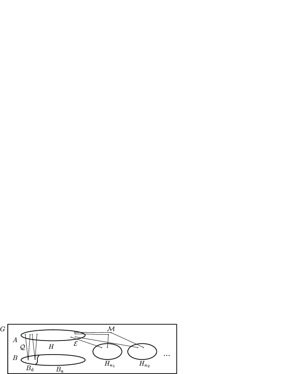
Figure 2: The situation in Lemma 3.8. Most of the set $T_{\ominus}$ is embedded in $A$, most of the set $T_{\oplus}$ will be embedded in $B$. The connections $\mathcal{E}$ and $\mathcal{M}$ are used to divert parts of $T$ to the graphs $H_{\kappa}$.

Lemma 3.8.

Suppose that $\alpha\in(0,\frac{1}{10})$ is arbitrary. For each tree $T\in\mathcal{T}_{k+1}$ with less than $\alpha k$ leaves the following holds. Suppose that a bipartite graph $H=(A,B;E)$ and graphs $\{H_{\kappa}\}_{\kappa\in I}$ (where $I$ is arbitrary) are pairwise vertex-disjoint subgraphs of a graph $G$ on vertex set $V$. Suppose that the following properties are fulfilled.

1. $\delta(H_{\kappa})>34\alpha k$ for each $\kappa\in I$.

2. $\delta_{G}(A)\geq k$.

3. There exists an $A-(\bigcup_{\kappa}(V(H_{\kappa})))$-matching $\mathcal{E}$, and a family $\mathcal{M}$ of pairwise vertex-disjoint $A-(V\setminus V(H))-(\bigcup_{\kappa}V(H_{\kappa}))$ paths. Moreover, $V(\mathcal{E})\cap V(\mathcal{M})=\emptyset$.

4. $|\mathcal{E}|+|\mathcal{M}|<\alpha k$.

5. $|A|+|\mathcal{E}|\geq|T_{\ominus}|$.

6. $|B|+|\mathcal{E}|+|\mathcal{M}|\geq|T_{\oplus}|-1$.

7. $\delta(A,B)\geq|B|-\alpha k$.

8. The set $B$ has a decomposition $B=B_{\mathrm{a}}\dot{\cup}B_{\mathrm{d}}$, $|B_{\mathrm{d}}|\leq\alpha k$, $\delta(B_{\mathrm{a}},A)\geq|A|-\alpha k$, and there exists a family $\mathcal{Q}$ of $|B_{\mathrm{d}}|$ pairwise vertex-disjoint $A-B_{\mathrm{d}}-A$ paths. Moreover, $V(\mathcal{Q})\cap(V(\mathcal{E})\cup V(\mathcal{M}))=\emptyset$.

Then, $T\subseteq G$.

The proof is given in the Appendix.

3.3 Specific notation

A graph $H$ is said to have the LKS-property (with parameter $k$) if at least half of its vertices have degree at least $k$, i. e., we have $|L|\geq\tfrac{v(H)}{2}$, where $L=\{v\in V(H)\>:\>\deg_{H}(v)\geq k\}$.

When we refer to $q,n_{0},n,k$ or $G$ in the rest of the paper, we always refer to the objects from the statement of Theorem 1.5. The vertex set of $G$ is denoted by $V$. We partition $V=L\dot{\cup}S$, where $L=\{v\in V\>:\>\deg(v)\geq k\}$ and $S=\{v\in V\>:\>\deg(v)<k\}$. We call the vertices from $L$ large and the vertices from $S$ small. The hypothesis of Theorem 1.5 implies that $|L|\geq\tfrac{n}{2}$. Finally $T$ denotes a tree of order $k+1$ that we want to embed in $G$.

We write $\alpha\ll\beta$ to express that $\alpha$ is sufficiently small compared to $\beta$.

4 Proof of the Main Theorem (Theorem 1.5)

The proof of Theorem 1.5 is based on an iterated application of Lemma 4.1 and 4.2 below. To state Lemma 4.1 we need to introduce the notion of $(\beta,\sigma)$-extremality. The $(\beta,\sigma)$-extremality says that a part of a graph resembles the extremal structure as in Figure 1. For two reals $\beta,\sigma\in(0,1)$, a partition of the vertex set $V=V_{1}\dot{\cup}V_{2}\dot{\cup}\ldots\dot{\cup}V_{\ell}\dot{\cup}\tilde{V}$ is $(\beta,\sigma)$-extremal if the following conditions are satisfied.

• $\ell\geq 1\;$.

• $(1-\beta)k\leq|V_{i}|\leq(1+\beta)k$ for each $i\in[\ell]\;$.

• $\tilde{V}=\emptyset$ or $|\tilde{V}|>\sigma k\;$.

• $e(V_{i},V\setminus V_{i})\leq\beta k^{2}$ for each $i\in[\ell]\;$, and $e(\tilde{V},V\setminus\tilde{V})\leq\beta k^{2}\;$.

• $(\tfrac{1}{2}-\beta)k\leq|V_{i}\cap L|$ for each $i\in[\ell]\;$.

• $|\tilde{V}\cap L|\leq(\tfrac{1}{2}-\sigma)|\tilde{V}|\;$.

Lemma 4.1 below, which will be proved in Section 7, deals with a graph that admits an extremal partition.

Lemma 4.1.

Given a number $q>0$, there exists a constant $c_{\mathbf{E}}>0$ such that the following holds. For each $\sigma\leq c_{\mathbf{E}}$ there exists a number $\beta\in(0,\sigma)$ such that if $G$ is a graph satisfying the LKS-property with $k\geq qn$ that admits a $(\beta,\sigma)$-extremal partition $V=V_{1}\dot{\cup}\ldots\dot{\cup}V_{\ell}\dot{\cup}\tilde{V}$, then $\mathcal{T}_{k+1}\subseteq G$, or there exists a set $Q\subseteq\tilde{V}$ such that

1. $|Q|>\tfrac{k}{2}\;$.

2. $|Q\cap L|>\tfrac{|Q|}{2}\;$.

3. $e(Q,V\setminus Q)<\sigma k^{2}\;$.

The next statement, which will be proved in Section 6, entails the regularity part of the proof of Theorem 1.5.

Lemma 4.2.

Given numbers $q,c,\rho>0$ there are numbers $\lambda\in(0,\rho)$ and $n_{0}=n_{0}(q,c,\rho)\in\mathbb{N}$ such that for each graph $G$ on $n\geq n_{0}$ vertices satisfying the LKS-property with $k\geq qn$ with a subset $V_{*}\subseteq V$ having the following properties

1. $|V_{*}|>ck\;$,

2. $e(V_{*},V\setminus V_{*})\leq\lambda k^{2}\;$, and

3. $|L\cap V_{*}|\geq\tfrac{1}{2}(1-\lambda)|V_{*}|\;$,

there exists a subset $V^{\prime}\subseteq V_{*}$ such that

• $(1-\rho)k\leq|V^{\prime}|\leq(1+\rho)k\;$,

• $|V^{\prime}\cap L|\geq\tfrac{1}{2}|V^{\prime}|\;$, and

• $e(V^{\prime},V\setminus V^{\prime})\leq\rho k^{2}\;$,

or $\mathcal{T}_{k+1}\subseteq G$.

Proof of Theorem 1.5.

Given $q>0$ let $c_{\mathbf{E}}$ be given by Lemma 4.1. Further let $\beta$ be given by Lemma 4.1 with input parameters $q,c_{\mathbf{E}}$ and $\sigma=c_{\mathbf{E}}$. Set $c=\frac{q\beta}{2}$ and $C=\lceil\frac{1}{q}\rceil$. We find a sequence of parameters

$$0<\sigma_{1}\ll\rho_{1}\ll\sigma_{2}\ll\rho_{2}\ll\dots\ll\rho_{C-1}\ll\sigma_{C}\ll\rho_{C}\;,$$ (4.1)

constructed as follows. Set $\rho_{C}=c$. Inductively for each $i=C,\dots,1$ let $\sigma_{i}=\lambda(q,c,\rho_{i})$ be given by Lemma 4.2 for input parameters $q,c$ and $\rho_{i}$. Further let $\beta_{i}$ be given by Lemma 4.1 with input parameters $q,c_{\mathbf{E}}$ and $\frac{\sigma_{i}}{2}$. Finally for $i>1$ set $\rho_{i-1}=\frac{\beta_{i}}{C}$. Set $n_{0}=\underset{i=1,\dots,C}{\max}\{n_{0}(q,c,\rho_{i})\}$, where the numbers $n_{0}(q,c,\rho_{i})$ are from Lemma 4.2.

Let $G$ be a graph satisfying the conditions of Theorem 1.5 (i.e., $q$ is fixed, $n\geq n_{0}$, and $k>qn$).

Recall that $\mathrm{ci}(x)$ denotes the closest integer to $x$. Let $\vartheta=\mathrm{ci}(\tfrac{n}{k})$. We iterate the following process for at most $\vartheta$ steps. In step $i,\;i\leq\vartheta$, we prove that $\mathcal{T}_{k+1}\subseteq G$ or we define a set $V_{i}\subseteq V\setminus\bigcup_{j<i}V_{j}$ such that the following conditions are fulfilled for each $j\in[i]$.

• $(1-\rho_{i})k\leq|V_{j}|\leq(1+\rho_{i})k$,

• $|L\cap V_{j}|\geq(\tfrac{1}{2}-\rho_{i})k$, and

• $e(V_{j},V\setminus V_{j})\leq\rho_{i}k^{2}$.

In step $i=1$, we apply Lemma 4.2 with parameters $q,c,\rho_{1}$ and input set $V_{*}=V$. We obtain that $\mathcal{T}_{k+1}\subseteq G$, or there exists a set $V_{1}$ satisfying (P1)₁, (P2)₁, and (P3)₁. In step $i>1$, suppose that we have sets $V_{1},\dots,V_{i-1}$ satisfying (P1)_i-1, (P2)_i-1, and (P3)_i-1. Set $V^{*}=V\setminus\bigcup_{j<i}V_{j}$.

First assume that $|V^{*}|>ck$. If $|L\cap V^{*}|\geq\tfrac{1}{2}(1-\sigma_{i})|V^{*}|$, the graph $G$ satisfies the conditions of Lemma 4.2 (with input parameters $q,c,\rho_{i}$ and input set $V_{*}=V^{*}$). Indeed, $|V^{*}|>ck$ by assumption, $e(V^{*},V\setminus V^{*})\leq(i-1)\rho_{i-1}k^{2}\leq\beta_{i}k^{2}<\sigma_{i}k^{2}$ because $V_{1},\ldots,V_{i-1}$ satisfy (P3)_i-1, and $|L\cap V^{*}|\geq\tfrac{1}{2}(1-\sigma_{i})|V^{*}|$ by assumption.

If $|L\cap V^{*}|<\tfrac{1}{2}(1-\sigma_{i})|V^{*}|$, then the partition $V=V_{1}\dot{\cup}\dots\dot{\cup}V_{i-1}\dot{\cup}V^{*}$ is $(C\rho_{i-1},\tfrac{\sigma_{i}}{2})$-extremal. Indeed,

• $i>1$;

• $(1-C\rho_{i-1})k\leq(1-\rho_{i-1})k\leq|V_{j}|\leq(1+\rho_{i-1})k\leq(1+C\rho_{i-1})k$ for each $j\leq i-1$ by (P1)_i-1;

• $|V^{*}|>ck\geq\tfrac{\sigma_{i}k}{2}$ by assumption;

• $e(V_{j},V\setminus V_{j})\leq\rho_{i-1}k^{2}\leq C\rho_{i-1}k^{2}$ for each $j\leq i-1$ by (P3)_i-1 and
  $e(V^{*},V\setminus V^{*})\leq(i-1)\rho_{i-1}k^{2}<C\rho_{i-1}k^{2}$;

• $|V_{j}\cap L|\geq(\tfrac{1}{2}-\rho_{i-1})k\geq(\tfrac{1}{2}-C\rho_{i-1})k$ for each $j\leq i-1$ by (P2)_i-1;

• $|V^{*}\cap L|<\tfrac{1}{2}(1-\sigma_{i})|V^{*}|=(\tfrac{1}{2}-\tfrac{\sigma_{i}}{2})|V^{*}|$.

Therefore Lemma 4.1 with parameters $q,c_{\mathbf{E}},\tfrac{\sigma_{i}}{2}$ applies. Thus $\mathcal{T}_{k+1}\subseteq G$, or there exists a set $Q\subseteq V^{*}$ satisfying Lemma 4.1 $(i)$–$(iii)$. It is enough to assume the latter case. Here again, the graph $G$ satisfies the conditions of Lemma 4.2 (with input parameters $q,c,\rho_{i}$ and input set $V_{*}=Q$). Indeed, $|Q|>\tfrac{k}{2}\geq\tfrac{q\beta}{2}k=ck$, $e(Q,V\setminus Q)<\tfrac{\sigma_{i}}{2}k^{2}<\sigma_{i}k^{2}$ and $|Q\cap L|>\tfrac{|Q|}{2}>\tfrac{1}{2}(1-\sigma_{i})|Q|$. Thus Lemma 4.2 yields that $\mathcal{T}_{k+1}\subseteq G$, or that there exists a set $V_{i}\subseteq Q$ satisfying Properties (P1)_i–(P3)_i.

It remains to deal with the case $|V^{*}|\leq ck$. The set $V$ is decomposed into sets $V_{1},\ldots,V_{i-1}$, each of which is of size approximately $k$, and a little set $V^{*}$. Thus, $i-1=\theta$. Having found sets $V_{1},\dots,V_{\vartheta}$ satisfying (P1)_ϑ–(P3)_ϑ, we set $V_{1}^{\prime}=V_{1}\cup V^{*}$ and $V_{j}^{\prime}=V_{j}$ for $j\geq 2$. The thus defined partition $V=V^{\prime}_{1}\dot{\cup}\dots\dot{\cup}V^{\prime}_{\vartheta}\dot{\cup}\emptyset$ is $(\beta,c_{\mathbf{E}})$-extremal. Indeed, by (P1)_ϑ–(P3)_ϑ, we have

• $\vartheta\geq 1$;

• $(1-\beta)k\leq(1-\rho_{\vartheta})k\leq|V_{j}|\leq|V^{\prime}_{j}|\leq|V_{j}|+|V^{*}|\leq(1+\rho_{\vartheta}+c)k\leq(1+\beta)k$ for each $j\leq\vartheta$;

• $e(V^{\prime}_{j},V\setminus V^{\prime}_{j})\leq e(V_{j},V\setminus V_{j})+e(V^{*},V\setminus V^{*})\leq\rho_{\vartheta}k^{2}+(\vartheta-1)\rho_{\vartheta}k^{2}\leq\beta k^{2}$ for each $j\leq\vartheta$ (the summand $e(V^{*},V\setminus V^{*})$ is necessary only when $j=1$);

• $|V^{\prime}_{j}\cap L|\geq|V_{j}\cap L|\geq(\tfrac{1}{2}-\rho_{\vartheta})k\geq(\tfrac{1}{2}-\beta)k$ for each $j\leq\vartheta$.

Lemma 4.1 with parameters $q,c_{\mathbf{E}}$ and $\sigma=c_{\mathbf{E}}$ yields that $\mathcal{T}_{k+1}\subseteq G$ (as no new set $Q$ can be found). ∎

5 Tools for the proof of Lemma 4.2

5.1 Sparsity in the set of large vertices

Suppose that $G$ is a graph with the LKS-property with parameter $k$ such that its set $L$ of large vertices is almost independent. In this section we provide an ad-hoc argument showing that in (a situation a bit more general than) the setting above, we have $\mathcal{T}_{k+1}\subseteq G$. Indeed, in this case $G$ is close to a $k$-regular bipartite graph with color classes $L$ and $S$, and thus we are roughly in the setting of Fact 3.6.

Lemma 5.1.

For every $q>0$ there exists a real $c_{\mathbf{S}}>0$ such that for each $c\in(0,c_{\mathbf{S}}]$ and each $n$-vertex graph $G=(V,E)$ with the LKS-property with parameter $k>qn$, and with a set $V_{*}\subseteq V$ satisfying

1. $|V_{*}|>\sqrt[4]{c}k\;$,

2. $e(V_{*},V\setminus V_{*})<ck^{2}\;$,

3. $(\tfrac{1}{2}-c)|V_{*}|<|V_{*}\cap L|\;$, and

4. $e(G[V_{*}\cap L])<cn^{2}\;$,

we have $\mathcal{T}_{k+1}\subseteq G$.

Proof.

Set $c_{\mathbf{S}}=q^{9}10^{-8}$. Let $c\in(0,c_{\mathbf{S}}]$ be arbitrary. Let $G$ be any graph satisfying the assumptions of the lemma. First observe that

$$|V_{*}|\geq\tfrac{3k}{4}\;.$$ (5.1)

Indeed, suppose the contrary. Assumptions $(i)$ and $(iii)$ imply that $|V_{*}\cap L|\geq(\tfrac{1}{2}-c)\sqrt[4]{c}k>\tfrac{1}{4}\sqrt[4]{c}k$. By the negation of (5.1), each vertex in $V_{*}\cap L$ emanates at least $\tfrac{k}{4}$ edges into $V\setminus V_{*}$. Therefore $e(V_{*}\cap L,V\setminus V_{*})>\tfrac{1}{16}\sqrt[4]{c}k^{2}$, a contradiction to $(ii)$.

Fix a set $L_{1}\subseteq L\cap V_{*}$ of size $|L_{1}|=(\tfrac{1}{2}-c)|V_{*}|$. Define $L_{2}=\{u\in L_{1}\>:\>\deg(u,V_{*}\setminus L_{1})\geq(1-2\sqrt{c})k\}$. For each vertex $x\in L_{1}\setminus L_{2}$ we have that $\deg(x,L_{1})+\deg(x,V\setminus V_{*})>2\sqrt{c}k$, otherwise $x$ would have been included in $L_{2}$. Summing up $(ii)$ and $(iv)$, we have $e(G[L_{1}])+e(L_{1}\setminus L_{2},V\setminus V_{*})<2cn^{2}$. Theorefore, we have that

$$|L_{1}\setminus L_{2}|\leq\frac{4cn^{2}}{2\sqrt{c}k}\overset{\mbox{\tiny{\eqref{eq:barVbig}}}}{<}3\sqrt{c}q^{-2}|V_{*}|\leq\frac{1}{2}\sqrt[4]{c}|V_{*}|\;.$$

Consequently,

$$|L_{2}|>(\tfrac{1}{2}-\sqrt[4]{c})|V_{*}|\;.$$ (5.2)

We verify that the set $\tilde{S}=\{u\in V_{*}\setminus L_{1}\>:\>\deg(u,L_{2})\geq(1-\sqrt[8]{c})k\}$ covers almost the whole set $V_{*}\setminus L_{1}$. Define $L_{*}=\{y\in V_{*}\setminus L_{1}\>:\>\deg(y,L_{2})\geq k\}$. Observe that $L_{*}\subseteq L\cap\tilde{S}$. By $(iv)$, less than $cn^{2}$ edges of $E[L_{2},V_{*}\setminus L_{1}]$ are incident with a vertex from $L_{*}$. Hence the number of edges in the bipartite graph $B=G[L_{2},V_{*}\setminus(L_{1}\cup L_{*})]$ is at least

$$e(B)\geq|L_{2}|(1-2\sqrt{c})k-cn^{2}\overset{\mbox{\tiny{\eqref{eqLtilBig},\eqref{eq:barVbig}}}}{\geq}(\tfrac{1}{2}-2\sqrt[4]{c})|V_{*}|k\;\mbox{.}$$ (5.3)

On the other hand, we upper-bound the number of edges in the graph $B$ using the fact that for each $x\in\tilde{S}\setminus L_{*}$ and for each $y\in V_{*}\setminus(L_{1}\cup\tilde{S})$ we have that $\deg_{B}(x)<k$ and $\deg_{B}(y)\leq(1-\sqrt[8]{c})k$, respectively.

$$e(B) \leq|\tilde{S}\setminus L_{*}|k+|V_{*}\setminus(L_{1}\cup\tilde{S})|(1-\sqrt[8]{c})k\qquad\big{[}\mbox{as $\tilde{S}\cup(V_{*}\setminus(L_{1}\cup\tilde{S}))=V_{*}\setminus L_{1}$}\big{]}$$

$$=|V_{*}\setminus L_{1}|k-\sqrt[8]{c}|V_{*}\setminus(L_{1}\cup\tilde{S})|k$$

$$=(\tfrac{1}{2}+c)|V_{*}|k-\sqrt[8]{c}|V_{*}\setminus(L_{1}\cup\tilde{S})|k\mbox{.}$$ (5.4)

Combining (5.3) with (5.4) we obtain

$$|V_{*}\setminus(L_{1}\cup\tilde{S})|\leq 3\sqrt[8]{c}|V_{*}|\leq\frac{3\sqrt[8]{c}k}{q}\;.$$ (5.5)

By the choice of $L_{2}$ and $\tilde{S}$, the minimum degree of the vertices in $L_{2}$ in the bipartite graph $G_{1}=G[L_{2},\tilde{S}]$ is at least $(1-2\sqrt{c})k-|V_{*}\setminus(L_{1}\cup\tilde{S})|$, and of those in $\tilde{S}$ at least $(1-\sqrt[8]{c})k$. By (5.5) and the choice of $c_{\mathbf{S}}$ we have that $\delta(G_{1})>\tfrac{k}{2}$.

Fact 3.6 applied on the graphs $B$ and $G$ yields that $\mathcal{T}_{k+1}\subseteq G$. ∎

5.2 Cutting trees, and (un)balanced trees

Definition 5.2.

An $\ell$-fine partition of a tree $T\in\mathcal{T}_{k+1}$ rooted at a vertex $R\in V(T)$ is a quaternary $\mathcal{D}=(W_{A},W_{B},\mathcal{D}_{A},\mathcal{D}_{B})$ with the following properties.

1. $W_{A}$ and $W_{B}$ are sets of vertices in $V(T)$. $\mathcal{D}_{A}$ and $\mathcal{D}_{B}$ are sets of subtrees in $T$. Further, $V(T)$ is a disjoint union of $W_{A}$, $W_{B}$, and the sets $V(t)$, $t\in\mathcal{D}_{A}\dot{\cup}\mathcal{D}_{B}$.

2. The distance from each vertex in $W_{A}$ to each vertex in $W_{B}$ is odd. The distance between each pair of vertices in $W_{A}$ or between each pair of vertices in $W_{B}$ is even.

3. No tree from $\mathcal{D}_{A}$ is adjacent to any vertex in $W_{B}$. No tree from $\mathcal{D}_{B}$ is adjacent to any vertex in $W_{A}$.

4. $v(t)\leq\ell$ for each tree $t\in\mathcal{D}_{A}\cup\mathcal{D}_{B}$.

5. $R\in W_{A}\cup W_{B}$.

6. $\max\{|W_{A}|,|W_{B}|\}\leq\frac{12k}{\ell}$.

7. $\mathcal{D}_{B}$ contains no internal tree.

8. We have

   $$\sum_{\begin{subarray}{c}t\in\mathcal{D}_{A}\\ t\textrm{ end-tree}\end{subarray}}v(t)\geq\sum_{t\in\mathcal{D}_{B}}v(t)\;\mbox{.}$$

9. Each internal tree from $\mathcal{D}_{A}$ is adjacent to two vertices of $W_{A}$.

For an $\ell$-fine partition $\mathcal{D}=(W_{A},W_{B},\mathcal{D}_{A},\mathcal{D}_{B})$ the trees from $\mathcal{D}_{A}\cup\mathcal{D}_{B}$ are called shrubs. For a subset $\mathcal{F}\subseteq\mathcal{D}_{A}\cup\mathcal{D}_{B}$, we denote the vertices contained in $\mathcal{F}$ by $V(\mathcal{F})$ and we write $v(\mathcal{F})=|V(\mathcal{F})|$.

It is proven in [23] that for every $\ell$ each tree can be cut up in a way which results in a partition that satisfies (i)–(viii) of Definition 5.2. Here we extend this result by the additional requirement of (ix) from Definition 5.2.

Lemma 5.3.

Let $T\in\mathcal{T}_{k+1}$ be a tree rooted at a vertex $R$ and let $\ell\in\mathbb{N},\ell<k$. Then the rooted tree $(T,R)$ has an $\ell$-fine partition.

For the proof, we shall need the following easy claim.

Fact 5.4 ([28, Proposition 7.11]).

Let $T$ be a tree with $\ell$ leaves. Then $T$ has at most $\ell-2$ vertices of degree at least three.

Proof of Lemma 5.3.

We first cut up the tree $T$ into components of order at most $\ell$. To this end we start with an empty set $W_{1}$ and place a token $v$ on the root $R$. At each step we check whether all the components of $T-v$ possibly except the one containing $R$ are of individual orders at most $\ell$. If that is the case then we insert $v$ into $W_{1}$, and we delete $v$ as well as all the said components from $T$. We restart with the token $v$ again on $R$. Otherwise, we move $v$ one vertex down to any component of order more than $\ell$. Obviously, at the stage when the process terminates, we have $|W_{1}|\leq\frac{k+1}{\ell+1}$. Last, we add $R$ to $W_{1}$. Then $|W_{1}|\leq\frac{k+1}{\ell+1}+1$.

Next, we want to refine the set of cut vertices $W_{1}$ in order to satisfy (ix) of Definition 5.2. To this end, consider the components $\mathcal{D}_{\geq 3}$ of $T-W_{1}$ that neighbour at least 3 vertices of $W_{1}$. Fix an arbitrary tree $t\in\mathcal{D}_{\geq 3}$. Let $X(t)\subseteq V(t)$ be the neighbors of $W_{1}$. Let $X^{\prime}(t)$ be all the vertices of $X(t)$ with the $\preceq$-maximal element removed. We have $|X^{\prime}(t)|=|X(t)|-1$. Consider the tree $\text{branch}(t)\subseteq t$ induced by the paths in $t$ connecting all the pairs of vertices of $X(t)$. Let $Y(t)$ be the vertices of degree at least 3 in $\text{branch}(t)$. By Fact 5.4, we have $|Y(t)|\leq|X(t)|-2<|X^{\prime}(t)|$. Observe that a map assigning to each vertex of $\bigcup_{t\in\mathcal{D}_{\geq 3}}X^{\prime}(t)$ any of its $\preceq$-minimal neighbors in $W_{1}$ is injective. Set $W_{2}=W_{1}\cup\bigcup_{t\in\mathcal{D}_{\geq 3}}Y(t)$. By the above, $|W_{2}|\leq|W_{1}|+\sum_{t\in\mathcal{D}_{\geq 3}}|X^{\prime}(t)|\leq 2|W_{1}|\leq\frac{2(k+1)}{\ell+1}+2$. Let $\mathcal{S}_{A}$ and $\mathcal{S}_{B}$ be a partition of all the components of $T-W_{2}$ where the respective membership of a component to $\mathcal{S}_{A}$ or to $\mathcal{S}_{B}$ is given by the parity of the distance of that component to $R$, and further such that

$$\sum_{\begin{subarray}{c}t\in\mathcal{S}_{A}\\ t\textrm{ end-tree}\end{subarray}}v(t)\geq\sum_{\begin{subarray}{c}t\in\mathcal{S}_{B}\\ t\textrm{ end-tree}\end{subarray}}v(t)\;\mbox{.}$$

In particular, we can write $W_{2}=W_{2A}\dot{\cup}W_{2B}$ where $W_{2A}$ are the parents of all the components of $\mathcal{S}_{A}$ and $W_{2B}$ are the parents of all the components of $\mathcal{S}_{B}$.

It remains to add further cut vertices in order to satisfy (iii) and (vii) of Definition 5.2. Initially, set $W_{3}=W_{2}$. For each internal tree $t_{B}\in\mathcal{S}_{B}$ we take its unique $\preceq$-maximal vertex and add it to the set $W_{3}$. Further, we add $\mathrm{Par}(W_{2B})\cap V(t_{B})$ to $W_{3}$. For each internal tree $t_{A}\in\mathcal{S}_{A}$ we add $\mathrm{Par}(W_{2B})\cap V(t_{A})$ to $W_{3}$. See Figure 3.

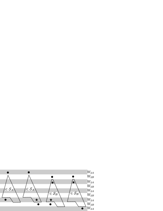
Figure 3: Obtaining the set $W_{3}$ from the set $W_{2}$ on examples of four internal trees depending on the parity of the neighbouring vertices of $W_{2}$ (which are denoted by dots). The newly added vertices are marked by stars.

As each vertex of $W_{2B}$ has at most one parent lying in some internal tree from $S_{A}\cup S_{B}$, we have

$$|W_{3}|\leq|W_{2}|+|\{\text{internal trees in $\mathcal{S}_{B}$}\}|+|W_{2B}|\;.$$

As each internal tree can be associated with a unique vertex of $W_{2}$ lying directly below it we get $|W_{3}|\leq 3|W_{2}|\leq\frac{6(k+1)}{\ell+1}+6\leq\frac{12k}{\ell}$. It is straightforward to check that the set $W_{3}$ partitioned according to the bipartite colouring $W_{3}=W_{A}\dot{\cup}W_{B}$ with the correspondingly partitioned components $\mathcal{D}_{A}\dot{\cup}\mathcal{D}_{B}$ of $T-W_{3}$ satisfies all requirements of Definition 5.2. ∎

The next lemma will allow us to remove trees which are locally unbalanced from further considerations in our proof of Theorem 1.5. Let us introduce the notion of (un)balanced forest now. For a real number $c\in(0,\tfrac{1}{2})$ we say that a family $\mathcal{C}$ of trees of total order at most $k+1$ is $c$-balanced if the forest formed by the trees $t\in\mathcal{C}$ with $|t_{\ominus}|>c\cdot v(t)$ is of order at least $ck$, i. e.,

$$\sum_{\begin{subarray}{c}t\in\mathcal{C}\\ |t_{\ominus}|>cv(t)\end{subarray}}v(t)\geq ck\;\mbox{.}$$

Otherwise, we say that $\mathcal{C}$ is $c$-unbalanced.

Note that when $\mathcal{C}$ is $c$-balanced, then

$$\sum_{t\in\mathcal{C}}|t_{\ominus}|\geq c^{2}k\;.$$ (5.6)

Lemma 5.5.

For each number $q>0$ there exists a constant $c_{\mathbf{U}}>0$ such that the following holds for each $n$-vertex graph $G$ with the LKS-property with parameter $k>qn$. Suppose that $T\in\mathcal{T}_{k+1}$ is given. If there exists a set $W\subseteq V(T)$, $|W|<c_{\mathbf{U}}k$ such that the family $\mathcal{C}$ of all components of the forest $T-W$ is $c_{\mathbf{U}}$-unbalanced, then $T\subseteq G$.

Proof.

Set $c_{\mathbf{U}}=\tfrac{c_{\mathbf{S}}}{6}$, where $c_{\mathbf{S}}$ is given by Lemma 5.1.

If the set $L$ induces less then $c_{\mathbf{S}}n^{2}$ edges then we have $T\subseteq G$ by Lemma 5.1 with $V_{*}=V$. In the rest we assume that $G[L]$ contains at least $c_{\mathbf{S}}n^{2}$ edges. A well-known fact asserts that there exists a graph $G^{\prime}\subseteq G[L]$ with minimum degree at least half of the average degree of $G[L]$, i. e., $\delta(G^{\prime})\geq c_{\mathbf{S}}n\geq 6c_{\mathbf{U}}(k+1)$.

Let $\mathcal{C}^{\prime}\subseteq\mathcal{C}$ be those trees $t\in\mathcal{C}$ for which $|t_{\ominus}|\leq c_{\mathbf{U}}v(t)$. Since $\mathcal{C}$ is $c_{\mathbf{U}}$-unbalanced we have $\sum_{t\in\mathcal{C}\setminus\mathcal{C}^{\prime}}v(t)<c_{\mathbf{U}}k$. Consequently,

$$\sum_{t\in\mathcal{C}^{\prime}}v(t)=v(T)-|W|-\sum_{t\in\mathcal{C}\setminus\mathcal{C}^{\prime}}v(t)>k+1-c_{\mathbf{U}}k-c_{\mathbf{U}}k>(1-2c_{\mathbf{U}})(k+1)\;.$$ (5.7)

Fact 3.2 gives that each tree $t\in\mathcal{C}^{\prime}$, $v(t)>1$ contains more than $(1-2c_{\mathbf{U}})v(t)$ leaves. The same property holds trivially for each tree $t\in\mathcal{C}^{\prime}$, $v(t)=1$. Employing (5.7), we get that there are at least $(1-2c_{\mathbf{U}})\sum_{t\in\mathcal{C}^{\prime}}v(t)\geq(1-4c_{\mathbf{U}})(k+1)$ leaves in the trees of $\mathcal{C}^{\prime}$. A leaf of a tree $t\in\mathcal{C}^{\prime}$ is either a leaf of $T$ or it is adjacent to a vertex in $W$. We root $T$ at an arbitrary vertex $r$, thus obtaining a partial order $\preceq$. Let $X$ be the set of vertices that are leaves of some tree $t\in\mathcal{C}^{\prime}$ but not leaves of $T$. Each vertex in $X$ is either a $\preceq$-minimal or a $\preceq$-maximal vertex of some tree $t\in\mathcal{C}$. Let $X_{\mathrm{min}}\subseteq X$ be the $\preceq$-minimal vertices and $X_{\mathrm{max}}=X\setminus X_{\mathrm{min}}$. (Note that the vertices which come out from $1$-vertex trees of $\mathcal{C}^{\prime}$ are included only in $X_{\mathrm{min}}$.) As each tree in $\mathcal{C}^{\prime}$ has a unique $\preceq$-maximal vertex we get $|X_{\mathrm{max}}|\leq h$, where $h$ is the number of trees in $\mathcal{C}^{\prime}$ which have order more than 1. Observe that each such tree has at least $\tfrac{1}{c_{\mathbf{U}}}$ vertices and thus $h\leq c_{\mathbf{U}}(k+1)$. For each $v\in X_{\mathrm{min}}$ we have $|\mathrm{Ch}(v)\cap W|\geq 1$. Since for each $u\in W$ it holds $|\mathrm{Par}(u)\cap X_{\mathrm{min}}|\leq 1$, we have $|X_{\mathrm{min}}|\leq|W|<c_{\mathbf{U}}k$. Summing the bounds we get $|X|<2c_{\mathbf{U}}(k+1)$. Thus $T$ has at least $(1-6c_{\mathbf{U}})(k+1)$ leaves. Therefore, we can apply Fact 3.7 on $G^{\prime}\subseteq G$ and conclude that $T\subseteq G$. ∎

5.3 A matching structure

A graph $H$ is said to be factor critical if for each its vertex $v$ the graph $H-v$ has a perfect matching. The following statement is a fundamental result in Matching theory. See [6, Theorem 2.2.3], for example.

Theorem 5.6 (Gallai–Edmonds Matching Theorem).

Suppose that $H$ is a graph. Then there exist a set $Q\subseteq V(H)$ and a matching $M$ of size $|Q|$ in $H$ such that every component of $H-Q$ is factor critical and the matching $M$ matches every vertex in $Q$ to a different component of $H-Q$.

The set $Q$ in Theorem 5.6 is called a separator. In order to introduce the main result of this section, Lemma 5.8, we need the following setting.

Setting 5.7.

Let $s>0$ and let $(H,\omega)$ be a weighted graph of order $N$, with $\omega:E(H)\rightarrow(0,s]$. Let $\sigma,K$ be two positive reals with $\tfrac{1}{2N}<\sigma<\min\{\tfrac{K}{32Ns},\tfrac{1}{30}\}$. Let $\mathcal{L}$ be a set of vertices such that

1. $V(H)\setminus\mathcal{L}$ is an independent set,

2. $|\mathcal{L}|>\tfrac{N}{2}-\sigma N$,

3. $\omega(u)\geq K$ for every $u\in\mathcal{L}$,

4. the set $\mathcal{L}$ induces at least one edge in $H$,

5. $\omega(u)<(1+\sigma)K$ for every $u\in V(H)\setminus\mathcal{L}$.

Lemma 5.8.

Let $s,N,\sigma,K,\mathcal{L}$, and a graph $(H,\omega)$ be as in Setting 5.7. Set $\mathcal{L}^{*}=\{u\in V(H)\>:\>\omega(u)\geq\tfrac{1}{2}(1+\sigma)K\}$. Then there exist a matching $M$ such that at least one of the following holds.

• There are two adjacent vertices $A,B\in V(H)\setminus V(M)$ with $A\in\mathcal{L}$, $\omega(A,V(M))\geq K-s$, and $\omega(B,V(M)\cup\mathcal{L}^{*})\geq\tfrac{1}{2}(1+\sigma)K$. For each edge $e\in M$ we have $|\mathrm{N}(A)\cap e|\leq 1$.

• There exists a set $\mathcal{O}\subseteq V(H)$ such that for each $x\in\mathcal{O}$ all but at most $2\sigma N$ neighbours of $x$ are covered by $M$. Furthermore, the set $\mathcal{O}\cap\mathcal{L}$ induces at least one edge, and $|V(M^{\prime})\setminus\mathcal{O}|\leq 1$, where $M^{\prime}=\{xy\in M\>:\>x,y\in\mathrm{N}(\mathcal{O})\}$.

Moreover, observe that each edge $e\in M$ intersects the set $\mathcal{L}$.

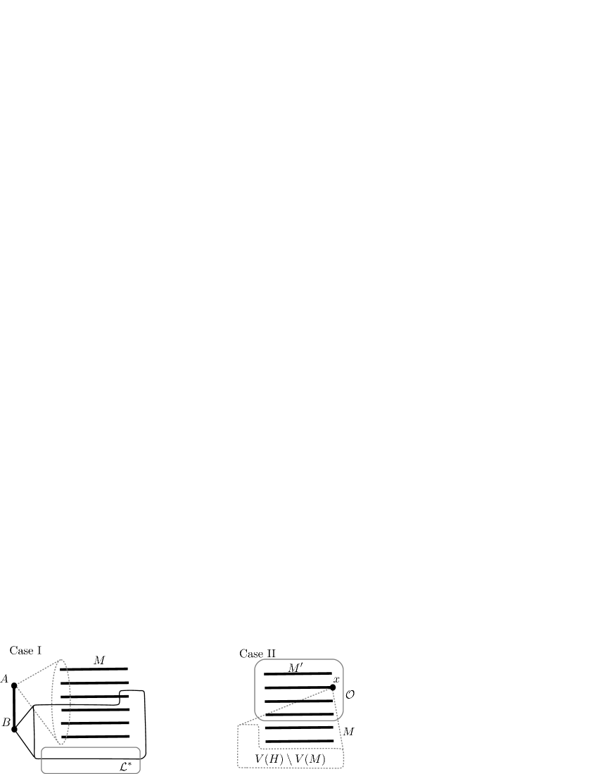
Figure 4: Two resulting matching structures from Lemma 5.8. Dashed lines represent no connections (in Case I), or sparse connections (in Case II).

Proof.

Among all the matchings satisfying the conclusion of Theorem 5.6, choose a matching $M_{0}$ that covers the maximum number of vertices from $V(H)\setminus\mathcal{L}^{*}$. Let $Q$ be the corresponding separator. By definition, $M_{0}$ is a $Q-(V(H)\setminus Q)$-matching. Set $\mathcal{L}_{0}=\mathcal{L}\setminus Q$ and $\mathcal{S}=V(H)\setminus\mathcal{L}$. We distinguish three cases.

$\bullet$  There exists an $\mathcal{L}_{0}-\mathcal{L}_{0}$ edge. Let $C$ be a component of $H-Q$ containing an $\mathcal{L}_{0}-\mathcal{L}_{0}$ edge. If $V(M_{0})\cap V(C)\not=\emptyset$, then we take $\{z\}=V(M_{0})\cap V(C)$. Otherwise, we choose $z$ arbitrarily in $C$. Since $C$ is factor critical, there exists a perfect matching $M_{1}$ in $C-z$. We claim that the conditions of Case II are satisfied for $M=M_{0}\cup M_{1}$, and $\mathcal{O}=V(C)$. Thus, $\mathcal{O}\cap\mathcal{L}$ induces an edge. Next, let $x\in\mathcal{O}$. We have $\mathrm{N}(x)\setminus\{z\}\subseteq V(M)$. Therefore, $\omega(x,V(M))\geq\omega(x)-s\geq\omega(x)-2\sigma Ns$. Consequently, all but at most $2\sigma N$ neighbours of $x$ are covered by $M$. To check that $|V(M^{\prime})\setminus\mathcal{O}|\leq 1$, it is enough to observe that each edge of $M^{\prime}$ except at most one is contained entirely in $C$.

$\bullet$  We have $\mathcal{L}_{0}=\emptyset$. Set $\mathcal{O}=V(H)$ and $M=M_{0}$. Setting 5.7 $(iv)$ implies that there is an edge in $\mathcal{O}\cap\mathcal{L}$. It is clear that $V(M^{\prime})\setminus\mathcal{O}=\emptyset$. Since $Q\supseteq\mathcal{L}$, $|\mathcal{L}|\geq\tfrac{N}{2}-\sigma N$, and $|V(M)|=2|Q|$ it holds that all but at most $2\sigma N$ vertices of $H$ are covered by $M$. The conditions of Case II are met.

$\bullet$  $\mathcal{L}_{0}$ is an independent set and $\mathcal{L}_{0}\not=\emptyset$. We first derive some auxiliary properties of the graph $H$.

Claim 5.8.1.

Each component $C$ of $H-Q$ is a singleton.

Proof.

Indeed, since $\mathcal{S}$ and $\mathcal{L}_{0}$ are independent, all the edges in each matching in $C$ are in the form $\mathcal{S}-\mathcal{L}_{0}$. Since $C$ is factor critical, we have $|V(C-u)\cap\mathcal{L}_{0}|=|V(C-u)\cap\mathcal{S}|$ for each vertex $u\in V(C)$. This is possible only when $v(C)=1$. ∎

Claim 5.8.1 implies that $M_{0}$ is a maximum matching in $H$. Define $\mathcal{\tilde{L}}=\{u\in\mathrm{N}(\mathcal{L}_{0})\>:\>\omega(u)\geq K\}$. Observe that $\mathcal{\tilde{L}}\subseteq Q$. By Setting 5.7 $(iii)$, we also have

$$\mathrm{N}(\mathcal{L}_{0})\setminus\tilde{\mathcal{L}}\subseteq Q\setminus\mathcal{L}\;.$$ (5.8)

Claim 5.8.2.

We have $\mathcal{\tilde{L}}\not=\emptyset$.

Proof.

Assume for contradiction that $\mathcal{\tilde{L}}=\emptyset$. Then for every vertex $u\in\mathrm{N}(\mathcal{L}_{0})$ we have $\omega(u)<K$. We get $|\mathcal{L}_{0}|K\leq\omega(\mathcal{L}_{0},\mathrm{N}(\mathcal{L}_{0}))<K|\mathrm{N}(\mathcal{L}_{0})|$ (the second inequality is indeed strict because $\mathrm{N}(\mathcal{L}_{0})\neq\emptyset$) implying

$$|\mathcal{L}_{0}|<|\mathrm{N}(\mathcal{L}_{0})|\;.$$ (5.9)

On the other hand, from $\mathcal{\tilde{L}}=\emptyset$ it follows that $\mathrm{N}(\mathcal{L}_{0})\cap\mathcal{L}=\emptyset$. Thus every vertex in $\mathrm{N}(\mathcal{L}_{0})$ is matched by $M_{0}$ to a distinct vertex in $\mathcal{L}_{0}$, a contradiction to (5.9). ∎

We show that the graph $V(H)$ fulfills the conditions of Case I. Suppose first that $B\in\mathrm{N}(\mathcal{L}_{0})$ is such that $\omega(B,V(M_{0})\cup\mathcal{L}^{*})\geq\tfrac{1}{2}(1+2\sigma)K$ and let $A\in\mathrm{N}(B)\cap\mathcal{L}_{0}$ be arbitrary. Set $M=M_{0}\setminus\{A,B\}$. It can then be easily shown that that pair $(A,B)$ satisfies the conditions of Case I.

So assume that for every $B\in\mathcal{\tilde{L}}\subseteq\mathrm{N}(\mathcal{L}_{0})$ we have

$$\omega(B,V(M_{0})\cup\mathcal{L}^{*}) <\tfrac{1}{2}(1+2\sigma)K\;\mbox{,}$$ (5.10)

which yields

$$\omega(B,X) >\tfrac{1}{2}(1-2\sigma)K\;\mbox{,}$$ (5.11)

where $X=V(H)\setminus(V(M_{0})\cup\mathcal{L}^{*})$.

Claim 5.8.3.

$M_{0}$ does not contain any edge with both end-vertices in $\mathcal{L}$.

Proof.

Indeed, suppose that such an edge $xy\in M_{0}$ exists. Then $x\in\mathcal{L}_{0}$ and $y\in\mathcal{\tilde{L}}$. By (5.11), $\omega(y,X)>\tfrac{1}{2}(1-2\sigma)K$. In particular, there exists a vertex $p\in\mathrm{N}_{X}(y)$. The matching $\{yp\}\cup M_{0}\setminus\{xy\}$ is a matching as in Theorem 5.6 (with separator $Q$) which covers more vertices of $V(H)\setminus\mathcal{L}^{*}$ than $M_{0}$. This contradicts the choice of $M_{0}$. ∎

Observe that for each vertex $u\in X$, we have $\omega(u,V(M))=\omega(u)<\tfrac{1}{2}(1+\sigma)K$. As $\mathcal{\tilde{L}}\subseteq V(M_{0})$, we have $\omega(u,\mathcal{\tilde{L}})<\tfrac{1}{2}(1+\sigma)K$. We bound $\omega(\mathcal{\tilde{L}},X)$ from both sides.

$$(1-2\sigma)|\mathcal{\tilde{L}}|\frac{K}{2}\overset{\eqref{eq_BinL*big}}{\leq}\omega(\mathcal{\tilde{L}},X)\leq(1+\sigma)|X|\frac{K}{2}\;\mbox{,}$$

which yields

$$|\mathcal{\tilde{L}}|\leq\frac{1+\sigma}{1-2\sigma}|X|\;\mbox{.}$$ (5.12)

We use (5.10) and $\mathcal{L}_{0}\subseteq\mathcal{L}^{*}$ to get $\omega(\tilde{\mathcal{L}},\mathcal{L}_{0})\leq|\tilde{\mathcal{L}}|(1+2\sigma)K/2$. Also, by the definition of $\tilde{\mathcal{L}}$, we have $\omega(\mathrm{N}(\mathcal{L}_{0})\setminus\tilde{\mathcal{L}},\mathcal{L}_{0})\leq K|\mathrm{N}(\mathcal{L}_{0})\setminus\tilde{\mathcal{L}}|$. Therefore,

$$|\mathcal{L}_{0}|K\leq\omega(Q,\mathcal{L}_{0}) \leq\omega(\mathcal{\tilde{L}},\mathcal{L}_{0})+\omega(\mathrm{N}(\mathcal{L}_{0})\setminus\tilde{\mathcal{L}},\mathcal{L}_{0})$$

$$\leq(1+2\sigma)\frac{K}{2}|\tilde{\mathcal{L}}|+K|\mathrm{N}(\mathcal{L}_{0})\setminus\tilde{\mathcal{L}}|$$

$$\overset{\eqref{eq:L0ALT}}{\leq}(1+2\sigma)\frac{K}{2}|\tilde{\mathcal{L}}|+K|Q\setminus\mathcal{L}|\;\mbox{,}$$

which gives

$$2|\mathcal{L}_{0}|\leq(1+2\sigma)|\mathcal{\tilde{L}}|+2|Q\setminus\mathcal{L}|\;\mbox{.}$$ (5.13)

Every vertex in $Q\setminus\mathcal{L}$ is matched with a vertex in $\mathcal{L}_{0}$. The converse is true due to Claim 5.8.3: if a vertex in $\mathcal{L}_{0}$ is matched then it is matched with a vertex in $Q\setminus\mathcal{L}$. Therefore, $|Q\setminus\mathcal{L}|=|\mathcal{L}_{0}\cap V(M_{0})|$. Combined with (5.13) we get that $2|\mathcal{L}_{0}\setminus V(M_{0})|\leq(1+2\sigma)|\mathcal{\tilde{L}}|$. Plugging in (5.12) we obtain

$$2|\mathcal{L}_{0}\setminus V(M_{0})|\leq\frac{(1+2\sigma)^{2}}{1-2\sigma}|X|\;\mbox{.}$$ (5.14)

By Setting 5.7 $(ii)$, we have $|\mathcal{L}|>|V(H)\setminus\mathcal{L}|-2\sigma N$. By Claim 5.8.3, we get $|\mathcal{L}_{0}\setminus V(M)|\geq|X|-2\sigma N$. Combined with (5.14) we obtain

$$2|X|-4\sigma N\leq\frac{(1+2\sigma)^{2}}{1-2\sigma}|X|\;\mbox{.}$$

We use the bounds $\sigma\leq\min\{\tfrac{K}{32Ns},\tfrac{1}{30}\}$ to get

$$|X|\leq\frac{4\sigma N}{1-14\sigma}\leq 8\sigma N\leq\frac{8K}{32s}\;\mbox{.}$$ (5.15)

On the other hand, using (5.11) and Claim 5.8.2, we get $\omega(\mathcal{\tilde{L}},X)>\frac{1}{2}(1-2\sigma)K|\mathcal{\tilde{L}}|$. As $\omega(e)\leq s$ for each $e\in E(H)$ we get $\omega(\mathcal{\tilde{L}},X)\leq s|\mathcal{\tilde{L}}||X|$. Combining these two bounds we arrive at

$$|X|>\frac{(1-2\sigma)K}{2s}>\frac{K}{4s}\;,$$

a contradiction to (5.15). ∎

5.4 Regularity Lemma

In this section we recall briefly the Regularity Lemma [27] and establish related notation. The reader may find more on the Regularity Method in [20, 19, 21].

Let $H=(V(H);E(H))$ be a graph. For two nonempty disjoint sets $X,Y\subseteq V(H)$ we denote the density of the pair $(A,B)$ by $\mathrm{d}(A,B)=\tfrac{e(A,B)}{|A||B|}.$ The pair $(A,B)$ is $\varepsilon$-regular, if for any subsets $X\subseteq A$, $Y\subseteq B$ with $|X|>\varepsilon|A|$ and $|Y|>\varepsilon|B|$, we have $|d(X,Y)-d(A,B)|<\varepsilon$. Such sets $X$ and $Y$ are called significant. We say that a vertex $v\in A$ is typical with respect to (“w. r. t.”) a significant set $Y\subseteq B$, if $\deg(v,Y)\geq(\mathrm{d}(A,B)-\varepsilon)|Y|$. Analogously, if $\{(A,B_{i})\}_{i=1}^{\ell}$ are $\varepsilon$-regular pairs, and $Y_{i}\subseteq B_{i}$ are significant, a vertex $v\in A$ is typical w. r. t. $\bigcup_{i-1}^{\ell}Y_{i}$, if $\deg(v,\bigcup_{i=1}^{\ell}Y_{i})\geq\sum_{i=1}^{\ell}(d(A,B_{i})-\varepsilon)|Y_{i}|$. Note that our definitions of typicality is only one-sided; this turns out to be sufficient for our proof.

Fact 5.9.

Let $X,Y_{1},Y_{2},\ldots,Y_{\ell}$ be disjoint sets of vertices, such that $(X,Y_{1}),(X,Y_{2}),\ldots,(X,Y_{\ell})$ are $\varepsilon$-regular pairs. Suppose that sets $W_{i}\subseteq Y_{i}$ are significant.

1. All but at most $\varepsilon|X|$ vertices of $X$ are typical w. r. t. $\bigcup_{i=1}^{\ell}W_{i}$.

2. All but at most $\sqrt{\varepsilon}|X|$ vertices of $X$ are typical w. r. t. at least $\sqrt{\varepsilon}\ell$ sets $W_{i}$.

The proof of $(ii)$ can be found in [28, Proposition 4.5]. We prove $(i)$ in the Appendix. The next fact is the well-known “slicing property” of regular pairs.

Fact 5.10 ([20, Fact 1.5]).

Suppose that $(X,Y)$ is an $\varepsilon$-regular pair of density $d$. Let $A\subseteq X$ and $B\subseteq Y$ be such that $|A|>\alpha|X|$, and $|B|>\alpha|Y|$ for $\alpha>2\varepsilon$. Then the pair $(A,B)$ is $\max\left\{\frac{\varepsilon}{\alpha},2\varepsilon\right\}$-regular of density at least $d-\varepsilon$.

A partition $V(H)=V_{0}\dot{\cup}V_{1}\dot{\cup}\ldots\dot{\cup}V_{N}$ of the vertex set a graph $H$ is called $(\varepsilon,N)$-regular if $|V_{0}|<\varepsilon v(H)$, $|V_{i}|=|V_{j}|$ for every $i,j\in[N]$, and for each $i\in[N]$ at most $\varepsilon N$ pairs $(V_{i},V_{j})$ (where $j\in[N]$) are not $\varepsilon$-regular. The sets $V_{1},\ldots,V_{N}$ are called clusters.

We are now ready to state a standard version Szemerédi’s original result [27].

Theorem 5.11 ([27]).

For every $\varepsilon>0$ and every $m_{0},r\in\mathbb{N}$, there exist numbers $M_{0},N_{0}\in\mathbb{N}$ such that every graph $H$ of order $m\geq N_{0}$ whose vertex sets is partitioned into $r$ sets $V(H)=O_{1}\dot{\cup}O_{2}\dot{\cup}\ldots\dot{\cup}O_{r}$ admits an $(\varepsilon,N)$-regular partition $V(H)=V_{0}\dot{\cup}V_{1}\dot{\cup}\ldots\dot{\cup}V_{N}$ for some $m_{0}\leq N\leq M_{0}$ such that for every $i\in[N]$ we have $V_{i}\subseteq O_{j}$ for some $j\in[r]$.

In the above setting, let $H_{d}$ denote the graph obtained from $H$ by deleting the edges incident to $V_{0}$, contained in some $V_{i}$, or in pairs of clusters that are irregular or of density smaller than some fixed constant $d$. Let $\mathbf{H}$ denote the cluster graph induced by $H_{d}$. That is, $\mathbf{H}$ has order $N$, its vertices are $V(\mathbf{H})=\{V_{1},\dots,V_{N}\}$ and edges are

$$E(\mathbf{H})=\{V_{i}V_{j}\>:\>(V_{i},V_{j})\mbox{ is a $\varepsilon$-regular pair with density at least $d$}\}\;\mbox{.}$$

Set $\mathrm{d\overline{eg}}_{\mathbf{H}}(C,D):=\mathrm{d\overline{eg}}_{H_{d}}(C,D)$, for any disjoint sets $C,D\subseteq V(H)$. The function $\mathrm{d\overline{eg}}_{\mathbf{H}}$ induces a weight function on $\mathbf{H}$.

5.5 Embedding lemmas

In this section, we introduce tools for embedding trees into regular pairs. Similar results are folklore. Here we give statements tailored to our needs; their proofs are included in the Appendix. The first lemma deals with embedding a tree into one regular pair.

Lemma 5.12.

Let $(t,r)$ be a rooted tree, and $d>2\varepsilon>0$. Let $(X,Y)$ be an $\varepsilon$-regular pair with $|X|=|Y|=s$ and density $\mathrm{d}(X,Y)\geq d$. Let $P^{\prime}\subseteq P\subseteq X$ and $Q^{\prime}\subseteq Q\subseteq Y$ be such that $\min\{|P|,|Q|\}\geq\Delta$ and $\max\{|P^{\prime}|,|Q^{\prime}|\}\geq\Delta$, where $\Delta\geq\frac{\varepsilon s+v(t)}{d-2\varepsilon}$. Then there exists an embedding $\phi$ of $t$ to $P\cup Q$ such that the root $r$ is mapped to $P^{\prime}\cup Q^{\prime}$. Moreover, if $|P^{\prime}|\geq\Delta$, the vertex $r$ can be mapped to $P^{\prime}$, and if $|Q^{\prime}|\geq\Delta$, the vertex $r$ can be mapped to $Q^{\prime}$.

The next lemma deals with embedding a tree using a matching structure in the underlying cluster graph. A simplified picture of the situation is given in Figure 5.

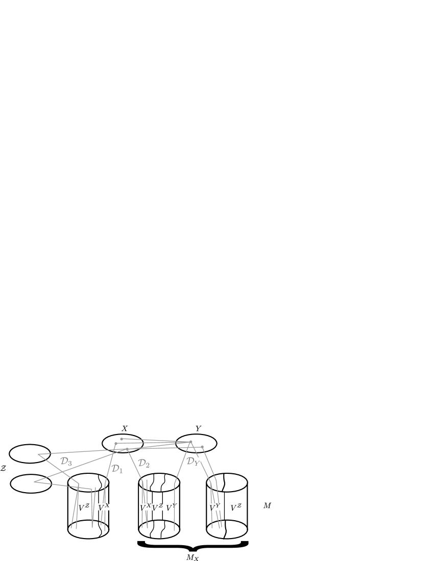
Figure 5: A simplified picture of an embedding provided by Lemma 5.13. The lemma provides with an embedding of a tree with a given fine partition $(W_{X},W_{Y},\mathcal{D}_{X},\mathcal{D}_{Y})$. The cut-vertices $W_{X}$ and $W_{Y}$ are mapped to $X$ and $Y$, respectively. The shrubs $\mathcal{D}_{Y}$ are mapped to the part $V^{Y}$ of the regular matching $M$. The shrubs $\mathcal{D}_{X}$ are embedded using one of three different ways which is indicated by the partition $\mathcal{D}_{X}=\mathcal{D}_{1}\dot{\cup}\mathcal{D}_{2}\dot{\cup}\mathcal{D}_{3}$. The shrubs of $\mathcal{D}_{1}$ are mapped to $V^{X}\setminus\bigcup V(M_{X})$. The shrubs of $\mathcal{D}_{2}$ which are required to be balanced are mapped to $V^{X}\cap\bigcup V(M_{X})$. Finally, the shrubs of $\mathcal{D}_{3}$ are accommodated to a set $V^{\mathcal{Z}}$ with their roots placed to an additional set of clusters $\mathcal{Z}$.

Lemma 5.13.

Let $0<\varepsilon,\xi,d\leq 1$ and $\tau,s$ be such that $\tau/s\leq\varepsilon\leq\xi^{2}d/400$. Let $F$ be a tree of order at most $k+1$ with a $\tau$-fine partition $(W_{X},W_{Y},\mathcal{D}_{X},\mathcal{D}_{Y})$ and let $\mathcal{D}_{1}\dot{\cup}\mathcal{D}_{2}\dot{\cup}\mathcal{D}_{3}$ be an arbitrary partition of $\mathcal{D}_{X}$. Let $\mathbf{H}$ be a cluster graph corresponding to an $\varepsilon$-regular partition of an $n$-vertex graph $H$, whose edges have density at least $d$ and clusters have size $s$. Let $XY\in E(\mathbf{H})$, and $X^{\prime}\subseteq X$, $Y^{\prime}\subseteq Y$ such that $|X^{\prime}|,|Y^{\prime}|\geq(1-d/2)s$. Let $\mathcal{Z}\subseteq V(\mathbf{H})\setminus\{X,Y\}$. Further let $M_{X}\subseteq M$ be matchings in $\mathbf{H}$ disjoint from $\mathcal{Z}\cup\{X,Y\}$ such that for each edge of $M_{X}$ contains at most one vertex of $\mathrm{N}_{\mathbf{H}}(X)$. Let $V^{X},V^{Y},V^{\mathcal{Z}}\subseteq\bigcup V(M)$ be pairwise disjoint sets. Suppose that

1. For all $CD\in M$, $|C\cap V^{X}|=|D\cap V^{X}|$, $|C\cap V^{Y}|=|D\cap V^{Y}|$, and $|C\cap V^{\mathcal{Z}}|=|D\cap V^{\mathcal{Z}}|$.

2. For all $C\in V(M)$, $|C\cap V^{X}|,|C\cap V^{Y}|,|C\cap V^{\mathcal{Z}}|\in\{0\}\cup(\varepsilon s,s]$.

3. If $\mathcal{D}_{Y}\neq\emptyset$, then $\mathrm{d\overline{eg}}_{\mathbf{H}}(Y,V^{Y})\geq v(\mathcal{D}_{Y})+\xi n$ .

4. If $\mathcal{D}_{1}\neq\emptyset$, then $\mathrm{d\overline{eg}}_{\mathbf{H}}(X,V^{X}\setminus\bigcup V(M_{X}))\geq v(\mathcal{D}_{1})+\xi n$ .

5. If $\mathcal{D}_{2}\neq\emptyset$, then $\mathcal{D}_{2}$ is $c$-balanced and $\mathrm{d\overline{eg}}_{\mathbf{H}}(X,V^{X}\cap\bigcup V(M_{X}))\geq v(\mathcal{D}_{2})-c^{2}k+\xi n$ .

6. If $\mathcal{D}_{3}\neq\emptyset$, then $\mathrm{d\overline{eg}}_{\mathbf{H}}(X,\bigcup\mathcal{Z})\geq|V(\mathcal{D}_{3})\cap\mathrm{N}_{F}(W_{X})|+\xi n$ .

7. If $\mathcal{D}_{3}\neq\emptyset$, then for each $Z\in\mathcal{Z}$, $\mathrm{d\overline{eg}}_{\mathbf{H}}(Z,V^{\mathcal{Z}})\geq v(\mathcal{D}_{3})+\xi n$ .

Then there is an embedding $\varphi$ of $F$ in $H$ such that $\varphi(W_{X})\subseteq X^{\prime}$, $\varphi(W_{Y})\subseteq Y^{\prime}$, $\varphi(V(\mathcal{D}_{Y}))\subseteq V^{Y}$, and $\varphi(V(\mathcal{D}_{X}))\subseteq(V^{X}\cup V^{\mathcal{Z}}\cup\bigcup\mathcal{Z})$.

6 Proof of Lemma 4.2

Suppose that $q,c$, and $\rho$ are given. Let $c_{\mathbf{S}}$ be given by Lemma 5.1 for input parameter $q$. Further, let $c_{\mathbf{U}}$ be given by Lemma 5.5 for input parameter $q$. Set reals $\zeta,\alpha,\gamma,\beta,\vartheta,\lambda,\kappa$ so that

$$0<\alpha\ll\beta\ll\gamma\ll\lambda\ll\zeta\ll\vartheta\ll\kappa\ll\min\{\rho,c,c_{\textbf{S}},c_{\mathbf{U}},q\}.$$

Let $n_{0}$ (the minimal order of the graph) and $\Pi_{1}$ (the upper bound for the number of clusters) be the numbers given by the Regularity Lemma 5.11 for input parameters $\alpha$ (for precision), $\Pi_{0}=\tfrac{2}{\alpha}$ (for the minimum number of clusters) and $4$ (for the number of pre-partition classes).

Let $G$ be a graph of order $n\geq n_{0}$ that has the LKS-property. We can assume that $G$ is LKS-minimal, that is, there is no proper spanning subgraph $G^{\prime}\subseteq G$ with the LKS-property. Then clearly,

$$\mbox{the set $S$ is independent}\;.$$ (6.1)

Let $V_{*}\subseteq V$ satisfy the assumptions of Lemma 4.2 and let $T\in\mathcal{T}_{k+1}$ be arbitrary. Our goal is to show that $T\subseteq G$. Root $T$ at an arbitrary vertex $R$, and consider any $\tau$-fine partition $(W_{A},W_{B},\mathcal{D}_{A},\mathcal{D}_{B})$ of $(T,R)$, with $\tau=\tfrac{\alpha k}{\Pi_{1}}$. The existence of such a partition follows from Lemma 5.3.

Prepartition the vertex set $V$ into $V_{*}\cap L,V_{*}\cap S,L\setminus V_{*}$, and $S\setminus V_{*}$. By the Regularity Lemma 5.11, there exists a partition $V=C_{0}\dot{\cup}C_{1}\dot{\cup}\dots\dot{\cup}C_{N}$ satisfying the following.

1. $\Pi_{0}\leq N\leq\Pi_{1}$,

2. $|C_{i}|=s$ for each $i\in[N]$,

3. $|C_{0}|\leq\alpha n$,

4. for each $i\in[N]$, all but at most $\alpha N$ pairs $(C_{i},C_{j})$ (where $j\in[N]$) are $\alpha$-regular,

5. for each $i\in[N]$, if $C_{i}\cap L\neq\emptyset$ then $C_{i}\subseteq L$, and if $C_{i}\cap V_{*}\neq\emptyset$ then $C_{i}\subseteq V_{*}$.

Let $G_{\gamma}$ denote the graph obtained from $G$ by deleting the edges incident to $C_{0}$, contained in some $C_{i}$, or in pairs of clusters that are irregular or of density smaller than $\gamma$ and let $\mathbf{G}$ be the corresponding cluster graph with weight function $\mathrm{d\overline{eg}}_{\mathbf{G}}$. Observe that by (R1)–(R4) we have

$$e(G_{\gamma})\geq e(G)-2\alpha n^{2}-\gamma n^{2}\geq e(G)-\lambda k^{2}\;.$$ (6.2)

Denote by $\mathcal{L}$ the set of clusters contained in $L\cap V_{*}$ which have large average degree in $V_{*}$:

$$\mathcal{L}=\{C\in V(\mathbf{G})\>:\>C\subseteq L\cap V_{*},\ \mathrm{d\overline{eg}}_{\mathbf{G}}(C,V_{*})\geq k-\sqrt{\lambda}n\}\;\mbox{.}$$

Note that (R5) supports the definition and observation below. Let $\mathcal{V}_{*}$ be the set of clusters contained in $V_{*}$; we write $N_{*}=|\mathcal{V}_{*}|$. Observe that each cluster inside $L\cap V_{*}$ is in $\mathcal{L}$, unless it sends many edges to $V\setminus V_{*}$. To estimate the size of $\mathcal{L}$, we set $\mathcal{B}=\{C\in V(\mathbf{G}):C\subseteq V_{*},\mathrm{d\overline{eg}}_{\mathbf{G}}(C,V\setminus V_{*})\geq\frac{\sqrt{\lambda}n}{2}\}$. It follows from the assumptions of Lemma 4.2 that

$$|\mathcal{B}|\leq 3\sqrt{\lambda}N\;.$$ (6.3)

Further, observe that we have

$$\mathcal{L}\supset\{C\in V(\mathbf{G}):C\subseteq V_{*}\cap L\}\setminus\mathcal{B}\;.$$ (6.4)

The ratio $|L\cap V_{*}|:|V_{*}|$ approximately corresponds to $|\mathcal{L}|:|\mathcal{V}_{*}|$. More precisely, we use later the following lower-bound on $|\mathcal{L}|$,

$$|\mathcal{L}|\geq\tfrac{1}{2}(1-2\lambda)N_{*}-|\mathcal{B}|\geq\tfrac{N_{*}}{2}-4\sqrt{\lambda}N\geq\tfrac{N_{*}}{2}-\zeta N_{*}\;,$$ (6.5)

where we use $\lambda\ll\zeta\ll c,q$.

Let $\mathbf{H}$ be the subgraph of $\mathbf{G}$ induced by $\mathcal{V}_{*}$ such that all the edges induced by the set $\mathcal{V}_{*}\setminus\mathcal{L}$ are removed. The cluster graph $\mathbf{H}$ naturally inherits the function $\mathrm{d\overline{eg}}_{\mathbf{G}}$ of $\mathbf{G}$ (which is denoted by $\mathrm{d\overline{eg}}_{\mathbf{H}}$). The next lemma gives some simple properties of $\mathbf{H}$.

Lemma 6.1.

 

1. For each $C\in\mathcal{L}$, we have $\sum_{D\in\mathrm{N}_{\mathbf{H}}(C)}\mathrm{d\overline{eg}}_{\mathbf{H}}(C,D)=\sum_{D\in\mathrm{N}_{\mathbf{G}}(C,V_{*})}\mathrm{d\overline{eg}}_{\mathbf{G}}(C,D)$.

2. All but at most $3\sqrt{\lambda}N$ clusters $C\in\mathcal{V}_{*}\setminus\mathcal{L}$ satisfy

   $$\sum_{D\in\mathrm{N}_{\mathbf{H}}(C)}\mathrm{d\overline{eg}}_{\mathbf{H}}(C,D)\geq\Big{(}\sum_{{D\in\mathrm{N}_{\mathbf{G}}(C,\mathcal{V}_{*})}}\mathrm{d\overline{eg}}_{\mathbf{G}}(C,D)\Big{)}-3\sqrt{\lambda}n\;.$$

Proof.

Part (i) follows directly. Let us now deal with part (ii). By (6.3), for any cluster $C\in\mathcal{V}_{*}\setminus(\mathcal{L}\cup\mathcal{B})$, we have $\mathrm{d\overline{eg}}_{\mathbf{H}}(C)\geq\mathrm{d\overline{eg}}_{\mathbf{G}}(C,V_{*})-|\mathcal{B}|s\geq\mathrm{d\overline{eg}}_{\mathbf{G}}(C,V_{*})-3\sqrt{\lambda}n$, as edges of $\mathbf{G}$ sent by $C$ go either to $\mathcal{B}$ or are kept in $\mathbf{H}$. At most $3\sqrt{\lambda}N$ clusters in $\mathcal{V}_{*}\setminus\mathcal{L}$ may be contained in $\mathcal{B}$. ∎

6.1 Matching structure in the cluster graph

Set $c^{\prime}=\min\{c_{\mathbf{S}},c^{4}\}$. If $e(G[V_{*}\cap L])<c^{\prime}n^{2}$, then the conditions of Lemma 5.1 are satisfied for the set $V_{*}$ and parameter $c_{\mathrm{L}\ref{prop_SCHolds}}=c^{\prime}$. Indeed, the assumptions $(i)$–$(iii)$ of Lemma 5.1 follow from the assumptions of Lemma 4.2, and the fact that $\lambda\ll c^{\prime}$. Then, by Lemma 5.1 we get $\mathcal{T}_{k+1}\subseteq G$. Therefore, we assume in the rest of the proof that $e(G[V_{*}\cap L])\geq c^{\prime}n^{2}$. By (6.2) as $\lambda\ll c^{\prime}$, we get $e(G_{\gamma}[V_{*}\cap L])\geq\frac{c^{\prime}}{2}n^{2}$.

Lemma 6.2.

The set $\mathcal{L}$ induces at least one edge in $\mathbf{H}$.

Proof.

By (6.4) and (6.3) at most $4\sqrt{\lambda}n^{2}$ of the edges of $E(G_{\gamma}[V_{*}\cap L])$ are not induced by the vertices of $\bigcup\mathcal{L}$. As $e(G_{\gamma}[V_{*}\cap L])\geq\frac{c^{\prime}}{2}n^{2}\gg 4\sqrt{\lambda}n^{2}$, $\mathcal{L}$ induces at least one edge in $\mathbf{G}$. This edge is also an edge in $\mathbf{H}$. ∎

The weighted graph $(\mathbf{H},\mathrm{d\overline{eg}}_{\mathbf{H}})$ satisfies the conditions of Lemma 5.8 with parameters $s$, $N=N_{*}$, $\sigma=\zeta$, and $K=k-\sqrt{\lambda}n$. Let us verify Conditions $(i)$–$(v)$ of Setting 5.7. Condition $(i)$ is satisfied by the way $\mathbf{H}$ was derived from $\mathbf{G}$. Condition $(ii)$ follows from (6.5). Condition $(iii)$ is given by the definition of $\mathcal{L}$. Condition $(iv)$ was derived in Lemma 6.2. Finally, Condition $(v)$ follows from the definitions of $L$ and $\mathcal{L}$. Lemma 5.8 ensures that one of the two specific matching structures in $\mathbf{H}$ exists.

Case I: There are two adjacent clusters $A,B$ and a matching $M$ in $\mathbf{H}-\{A,B\}$ such that:

1. We have $\mathrm{d\overline{eg}}_{\mathbf{H}}(A,V(M))\geq k-2\sqrt{\lambda}n$.

2. For each edge $e\in M$ we have $|\mathrm{N}_{\mathbf{H}}(A)\cap e|\leq 1$.

3. There is a set $\mathcal{L}^{*}\in V(\mathbf{H})$ such that for all $C\in\mathcal{L}^{*}$ we have $\mathrm{d\overline{eg}}_{\mathbf{H}}(C)\geq(1+\tfrac{\zeta}{2})\frac{k}{2}$ and

   $$\mathrm{d\overline{eg}}_{\mathbf{H}}(B,V(M)\cup\mathcal{L}^{\ast})\geq(1+\tfrac{\zeta}{2})\frac{k}{2}\;.$$ (6.6)

Case II: There exist a set of clusters $\mathcal{O}\subseteq V(\mathbf{H})$ and a matching $M$ in $\mathbf{H}$ such that:

1. $\mathcal{O}\cap\mathcal{L}$ induces at least one edge in $\mathbf{H}$.

2. $|V(M_{\mathcal{O}})\setminus\mathcal{O}|\leq 1$, where $M_{\mathcal{O}}=\{CD\in M\>:\>C,D\in\mathrm{N}_{\mathbf{H}}(\mathcal{O})\}$.

3. All clusters of $\mathcal{O}\cap\mathcal{L}$ and all but at most $3\sqrt{\lambda}N$ clusters $C\in\mathcal{O}\setminus\mathcal{L}$ satisfy

   $$\mathrm{d\overline{eg}}_{\mathbf{H}}(C,V(M))\geq\mathrm{d\overline{eg}}_{\mathbf{G}}(C,V_{*})-3\zeta n\;.$$

   To see this, recall that by the assertion of Lemma 5.8 we have that

   $$\sum_{D\in\mathrm{N}_{\mathbf{H}}(C)\cap V(M)}\mathrm{d\overline{eg}}_{\mathbf{H}}(C,D)\geq\sum_{D\in\mathrm{N}_{\mathbf{H}}(C)}\mathrm{d\overline{eg}}_{\mathbf{H}}(C,D)-2\zeta n$$

   for each $C\in\mathcal{O}$. Thus the assertion follows from Lemma 6.1.

4. Each edge of $M$ intersects $\mathcal{L}$.

We partition $\mathcal{D}_{A}=\mathcal{T}_{F}\dot{\cup}\mathcal{T}_{A}$, where $\mathcal{T}_{F}$ are the internal shrubs and by $\mathcal{T}_{A}$ are the end-shrubs of $\mathcal{D}_{A}$. Recall that $\mathcal{D}_{B}$ contains only end-shrubs and that $v(\mathcal{D}_{B})\leq v(\mathcal{T}_{A})$. We shall assume that $\mathcal{T}_{F}\cup\mathcal{T}_{A}\cup\mathcal{D}_{B}$ is $c_{\mathbf{U}}$-balanced, otherwise $T\subseteq G$ by Lemma 5.5.

As we shall show shortly, the proof of Lemma 4.2 follows from the following three statements, proofs of which are postponed to subsequent sections.

Lemma 6.3.

If we have Case I, then $T\subseteq G$.

Lemma 6.4.

If we have Case II, then $T\subseteq G$, or for any two clusters $A,B\in\mathcal{O}\cap\mathcal{L}$ that are adjacent in $\mathbf{H}$, there exists a matching $M_{A}\subseteq M-\{A,B\}$ such that $M_{A}$ and $V_{A}=\bigcup V(M_{A})$ satisfy the following properties.

1. $\mathrm{d\overline{eg}}_{\mathbf{H}}(A,C),\mathrm{d\overline{eg}}_{\mathbf{H}}(A,D)>(1-2\vartheta)s$ and $\mathrm{d\overline{eg}}_{\mathbf{H}}(A,CD)>(2-3\vartheta)s$, for all $CD\in M_{A}$.

2. $\mathrm{d\overline{eg}}_{\mathbf{H}}(A,V(M_{A}))\geq(1-8\vartheta)k$.

3. $(1-8\vartheta)k\leq|V_{A}|\leq k$.

4. $V(M_{A})\subseteq\mathcal{O}$.

5. If $v(\mathcal{D}_{B})\geq\sqrt[4]{\zeta}k$, then $\mathrm{d\overline{eg}}_{\mathbf{H}}(B,V(M_{A}))\geq(1-9\vartheta)k$.

6. If $v(\mathcal{D}_{B})<\sqrt[4]{\zeta}k$, then there exists a matching $M_{B}\subseteq M-(V(M_{A})\cup\{A,B\})$ such that $|M_{B}|\leq\sqrt[4]{\zeta}N$ and $v(\mathcal{D}_{B})+\lambda k\leq\mathrm{d\overline{eg}}_{\mathbf{H}}(B,V(M_{B}))\leq v(\mathcal{D}_{B})+\lambda k+2s$.

7. $|V_{A}\cap L|\geq\frac{1}{2}|V_{A}|$.

Lemma 6.5.

Suppose we have Case II and let $A,B\in\mathcal{O}\cap\mathcal{L}$, $AB\in E(\mathbf{H})$. Suppose that $M_{A}$, $M_{B}$ and $V_{A}$ satisfy $(i)$–$(vii)$ from Lemma 6.4. (For convenience, we take $M_{B}=\emptyset$ if the assumption of Lemma 6.4 $(vi)$ is not satisfied.) If $|e_{G_{\gamma}}(V_{A},V\setminus V_{A})|\geq\frac{\kappa n^{2}}{2}$, then $T\subseteq G$.

Given Lemmas 6.3–6.5, Lemma 4.2 follows. Indeed, we get that $\mathcal{T}_{k+1}\subseteq G$, or $e_{G_{\gamma}}(V_{A},V\setminus V_{A})<\kappa^{2}n^{2}/2$, with $V_{A}$ from Lemma 6.4. In the latter case, the assertions of Lemma 4.2 are fullfilled with the set $V^{\prime}:=V_{A}$. Indeed, by Lemma 4.2 $(ii)$ and by (6.2), we have $e_{G}(V_{A},V\setminus V_{A})\leq e_{G}(V_{*},V\setminus V_{*})+e_{G_{\gamma}}(V_{A},V\setminus V_{A})+e(G)-e(G_{\gamma})\leq 2\lambda k^{2}+\kappa n^{2}/2\ll\rho k^{2}$.

6.2 Proof of Lemma 6.3

We shall partition each cluster $C\in V(\mathbf{H})$ so that the partition defines two disjoint sets $V^{F},V^{B}\subseteq V(G)$. The embedding $\varphi:V(T)\rightarrow V(G)$ of $T$ will be defined in three phases. In the first phase, we shall embed the subtree $T^{\prime}=T[W_{A}\cup W_{B}\cup V(\mathcal{T}_{F}\cup\mathcal{T}^{M}_{B})]$, where $\mathcal{T}_{B}^{M}\subseteq\mathcal{D}_{B}$ will be defined later. The trees $\mathcal{T}_{F}$ will be embedded in $V^{F}$ and the trees $\mathcal{T}^{M}_{B}$ in $V^{B}$. In the second phase, we shall embed $\mathcal{T}_{B}^{L}=\mathcal{D}_{B}\setminus\mathcal{T}_{B}^{M}$ in $V^{B}$. In the last phase, we shall embed $\mathcal{T}_{A}$ in $V(G)$. From now on, we write $\varphi$ for the partial embedding (at the current stage) of $T$.

The difference between the present proof of Theorem 1.5 and its approximate version Theorem 1.4 is that in the proof of Theorem 1.5 we have to fight to gain back small loses caused by the use of the Regularity Lemma. However, this is not necessary when we have the matching structure of Case I. Indeed, we can reduce this situation to the “approximate version”, i.e., to a setting of similar nature as in Theorem 1.4.

Preparation.

We partition each cluster $C\in V(\mathbf{H})$ into sets $C^{F}$ and $C^{B}$ in an arbitrary way so that $|C^{F}|=(1-y)|C|$ and $|C^{B}|=y|C|$, where

$$y=\frac{v(\mathcal{T}_{A}\cup\mathcal{D}_{B})}{k}\cdot\frac{1}{1+\tfrac{\zeta}{4}}+\lambda\geq\frac{2v(\mathcal{D}_{B})}{k}\cdot\frac{1}{1+\tfrac{\zeta}{4}}+\lambda.$$ (6.7)

Note that

$$1-y \geq\frac{v(\mathcal{T}_{F})}{k}+\frac{\zeta}{8}\cdot\frac{v(\mathcal{T}_{A}\cup\mathcal{D}_{B})}{k}-\lambda$$ (6.8)

$$\geq\frac{v(\mathcal{T}_{F})}{k}-\lambda\;.$$ (6.9)

Set

$$V^{B}=\bigcup_{C\in V(\mathbf{H})}C^{B}\;,\quad V^{F}=\bigcup_{C\in V(\mathbf{H}}C^{F}\;,$$

$$M^{B}=V^{B}\cap\bigcup V(M)\;,\quad M^{F}=V^{F}\cap\bigcup V(M)\;\mbox{, and }\quad L^{B}=V^{B}\cap\bigcup(\mathcal{L}^{*}\setminus\{A,B\})\;\mbox{.}$$

Observe that (6.7) gives $y\in(\lambda,1-\lambda)$. Indeed, the lower bound is trivial and the upper bound follows from $\frac{1}{1+\frac{\zeta}{4}}<1-2\lambda$.

Let $\mathcal{T}^{M}_{B}\subseteq\mathcal{D}_{B}$ be a maximal subject to

$$\sum_{t\in\mathcal{T}^{M}_{B}}v(t)\leq\mathrm{d\overline{eg}}_{\mathbf{H}}(B,M^{B})-{\lambda n}.$$ (6.10)

Let $\mathcal{T}_{B}^{L}=\mathcal{D}_{B}\setminus\mathcal{T}_{B}^{M}$. From the maximality, we have

$$\sum_{t\in\mathcal{T}^{M}_{B}}v(t)\geq\mathrm{d\overline{eg}}_{\mathbf{H}}(B,M^{B})-{\lambda n}-\tau k\quad\mbox{or}\quad\mathcal{T}_{B}^{L}=\emptyset\;.$$ (6.11)

We now proceed with the three-phase embedding outlined above.

Phase 1 of the embedding.

Let $A^{\prime}\subseteq A$ be the set of typical vertices w. r. t. all but at most $\beta N$ sets $C\in V(M)$ and let  $B^{\prime}\subseteq B$ be the set of typical vertices w. r. t. $L^{B}$. From Fact 5.9,

$$\min\{|A^{\prime}|,|B^{\prime}|\}\geq(1-\sqrt{\alpha})s\;.$$ (6.12)

We use Lemma 5.13 to embed the tree $T^{\prime}=T[W_{A}\cup W_{B}\cup V(\mathcal{T}_{F}\cup\mathcal{T}^{M}_{B})]$ with the following setting. The cluster graph is $\mathbf{H}$, with $AB\in E(\mathbf{H})$ and $A^{\prime}\subseteq A$, $B^{\prime}\subseteq B$. The set $\mathcal{Z}$ is empty. The tree $T^{\prime}$ has a $\tau$-fine partition $(W_{A},W_{B},\mathcal{T}_{F},\mathcal{T}^{M}_{B})$. We have disjoint sets $M^{F}\dot{\cup}M^{B}\dot{\cup}\emptyset\subseteq\bigcup V(M)$. The sets $M^{F}$, $M^{B}$ and $\emptyset$ play the roles of $V^{X}$, $V^{Y}$, and $V^{\mathcal{Z}}$ from Lemma 5.13. If $\mathcal{T}_{F}$ is $c_{\mathbf{U}}/2$-balanced, we set $\mathcal{D}_{2}=\mathcal{T}_{F}$, $\mathcal{D}_{1}=\mathcal{D}_{3}=\emptyset$ and $M_{X}=M$. If $\mathcal{T}_{F}$ is not $c_{\mathbf{U}}/2$-balanced, we set $\mathcal{D}_{1}=\mathcal{T}_{F}$, $\mathcal{D}_{2}=\mathcal{D}_{3}=\emptyset$, and $M_{X}=\emptyset$. In particular, note that

$$\varphi(V(T^{\prime})\setminus V(\mathcal{T}_{B}^{M}))\cap M^{B}=\emptyset\;.$$ (6.13)

We now verify the assumptions of Lemma 5.13, where we use $d_{\mathrm{L\ref{lem:Embedding-3}}}=\gamma,\xi_{\mathrm{L\ref{lem:Embedding-3}}}=\lambda,\varepsilon_{\mathrm{L\ref{lem:Embedding-3}}}=\alpha$. The parameters $0<\alpha\ll\lambda\ll\gamma<1$ and $\tau,s$ satisfy $\tau/s<\alpha<\lambda^{2}\gamma/400$. The bound (6.12) guarantees that $A^{\prime}$ and $B^{\prime}$ have sizes as required by the lemma. Condition $(i)$ follows from the way $V^{F}$ and $V^{B}$ were defined and Condition $(ii)$ holds as $y\in(\lambda,1-\lambda)$. Conditions $(vi)$ and $(vii)$ hold trivially. Condition $(iii)$ follows from (6.10). If $\mathcal{T}_{F}$ is $c_{\mathbf{U}}/2$-balanced, Condition $(iv)$ holds trivially and for Condition $(v)$ observe that

$$\mathrm{d\overline{eg}}_{\mathbf{H}}(A,M^{F}) \geq(1-y)(\mathrm{d\overline{eg}}_{\mathbf{H}}(A,V(M))-\alpha n\;\qquad\text{[by~{}\eqref{eq:1-y} and Case~{}I\ref{hippiA}]}$$

$$\geq v(\mathcal{T}_{F})-3\sqrt{\lambda}n\geq v(\mathcal{T}_{F})-\tfrac{c_{\mathbf{U}}^{2}}{4}k+\lambda n\;.$$

As $\mathcal{T}_{A}\cup\mathcal{T}_{F}\cup\mathcal{D}_{B}$ is $c_{\mathbf{U}}$-balanced we get that if $\mathcal{T}_{F}$ is not $c_{\mathbf{U}}/2$-balanced then $\mathcal{T}_{A}\cup\mathcal{D}_{B}$ is $c_{\mathbf{U}}/2$-balanced. Condition $(v)$ holds trivially and for Condition $(iv)$ observe that

$$\mathrm{d\overline{eg}}_{\mathbf{H}}(A,M^{F}) \geq(1-y)(\mathrm{d\overline{eg}}_{\mathbf{H}}(A,V(M))-\alpha n\;\qquad\text{[by~{}\eqref{eq:1-ystronger} and Case~{}I\ref{hippiA}]}$$

$$\geq v(\mathcal{T}_{F})+v(\mathcal{T}_{A}\cup\mathcal{D}_{B})\frac{\zeta}{8}-3\sqrt{\lambda}n\geq v(\mathcal{T}_{F})+\lambda n\;.$$

Phase 2 of the embedding.

Phase 2 is skipped when $\mathcal{T}_{B}^{L}=\emptyset$. We label the shrubs of $\mathcal{T}_{B}^{L}$ as $t_{1},\ldots,t_{|\mathcal{T}_{B}^{L}|}$. In step $i\geq 1$, we define the embedding for the shrub $t_{i}$ in a suitable edge $CD\in E(\mathbf{G})$. Set $U_{i}=\varphi(V(\mathcal{T}_{F}\cup\mathcal{T}_{B}^{M})\cup\bigcup_{j<i}V(t_{j})).$ Let $x_{i}\in W_{B}$ be the parent of the root of the shrub $t_{i}$. The vertex $\varphi(x_{i})$ is typical w. r. t. $L^{B}$ and hence by (6.6), (6.7) and (6.11), we have

$$\deg(\varphi(x_{i}),L^{B}) \geq\mathrm{d\overline{eg}}_{\mathbf{H}}(B,L^{B})-\alpha n\geq\mathrm{d\overline{eg}}_{\mathbf{H}}(B,M^{B}\cup L^{B})-\mathrm{d\overline{eg}}_{\mathbf{H}}(B,M^{B})-\alpha n$$

$$\geq v(\mathcal{D}_{B})+\tfrac{\zeta k}{4}-v(\mathcal{T}_{B}^{M})-\lambda n-\tau k-2\alpha n\geq v(\mathcal{T}_{B}^{L})+\lambda n\;.$$

Thus there is a cluster $C\in\mathcal{L}^{*}$ with

$$|\mathrm{N}(\varphi(x_{i}))\cap C\setminus U_{i}|\geq\frac{\lambda n}{N}\geq\frac{\alpha s+\tau}{\gamma-2\alpha}\;.$$

From the definition of $\mathcal{L}^{*}$, (6.7), and (6.13) we obtain

$$\mathrm{d\overline{eg}}_{\mathbf{H}}(C,V^{B}\setminus U_{i})\geq\mathrm{d\overline{eg}}_{\mathbf{H}}(C,V^{B})-|\varphi(V(\mathcal{D}_{B}))\cap U_{i}|\geq\tfrac{\lambda k}{4}\;.$$

Therefore there is a cluster $D\in\mathrm{N}_{\mathbf{H}}(C)$ with $|D\setminus U_{i}|\geq\frac{\alpha s+\tau}{\gamma-2\alpha}$. We use Lemma 5.12 to embed $t_{i}$ in $(C\cup D)\setminus U_{i}$ so that the root of the shrub $t_{i}$ is mapped to $\mathrm{N}(\varphi(x_{i}))\cap C\setminus U_{i}$.

Phase 3 of the embedding.

We label $\mathcal{T}_{A}$ as $t_{1},\dots,t_{|\mathcal{T}_{A}|}$. In step $i=1,\dots,|\mathcal{T}_{A}|$, we define the embedding for the shrub $t_{i}$. Let $x_{i}\in W_{A}$ be the parent of the root $r_{i}$ of $t_{i}$. Set $U_{i}=\varphi(V(\mathcal{T}_{F}\cup\mathcal{D}_{B})\cup\bigcup_{j<i}V(t_{j}))$. For an edge $CD\in M$ with $C\in\mathrm{N}_{\mathbf{H}}(A)$ we define

$$\Upsilon^{i}_{CD}=\min\{|\mathrm{N}(\varphi(x_{i}))\cap C\setminus U_{i}|,|D\setminus U_{i}|\}\;.$$

By Lemma 5.12, the shrub $t_{i}$ can be embedded in unused vertices of an edge $CD\in M$ so that $r_{i}$ is mapped to a neighbor of $\varphi(x_{i})$, whenever $CD$ satisfies $\Upsilon^{i}_{CD}\geq\lambda s$. If $\mathcal{T}_{F}\cup\mathcal{D}_{B}$ is $\tfrac{c_{\mathbf{U}}}{2}$-balanced then by (5.6) we have

$$\sum_{\begin{subarray}{c}CD\in M\\ C\in\mathrm{N}_{\mathbf{H}}(A)\end{subarray}}\max\{|C\cap U_{i}|,|D\cap U_{i}|\}\leq v(\mathcal{T}_{A})+v(\mathcal{T}_{F}\cup\mathcal{D}_{B})-\sum_{t\in\mathcal{T}_{F}\cup\mathcal{D}_{B}}|t_{\ominus}|\leq v(\mathcal{T}_{A})+v(\mathcal{T}_{F}\cup\mathcal{D}_{B})-\tfrac{c_{\mathbf{U}}^{2}k}{4}\;.$$

By Fact 5.9 we have

$$\sum_{\begin{subarray}{c}CD\in M\\ C\in\mathrm{N}_{\mathbf{H}}(A)\end{subarray}}\Upsilon^{i}_{CD}\geq \sum_{\begin{subarray}{c}CD\in M\\ C\in\mathrm{N}_{\mathbf{H}}(A)\end{subarray}}\left(|\mathrm{N}(\varphi(x_{i}))\cap C|-\max\{|C\cap U_{i}|,|D\cap U_{i}|\}\right)$$

$$\geq \mathrm{d\overline{eg}}_{\mathbf{H}}(A,V(M))-2\sqrt{\alpha}n-(v(\mathcal{T}_{F}\cup\mathcal{D}_{B})-\tfrac{c_{\mathbf{U}}^{2}k}{4})-v(\mathcal{T}_{A})\geq\lambda n\;.$$

If $\mathcal{T}_{F}\cup\mathcal{D}_{B}$ is $\tfrac{c_{\mathbf{U}}}{2}$-unbalanced, then $\mathcal{T}_{A}$ is $\tfrac{c_{\mathbf{U}}}{2}$-balanced. Then by (5.6), $\max\{|V(\mathcal{T}_{A})\cap T_{\oplus}|,|V(\mathcal{T}_{A})\cap T_{\ominus}|\}\leq v(\mathcal{T}_{A})-(\tfrac{c_{\mathbf{U}}}{2})^{2}k$. We get

$$\sum_{\begin{subarray}{c}CD\in M\\ C\in\mathrm{N}_{\mathbf{H}}(A)\end{subarray}}\Upsilon^{i}_{CD}\geq \sum_{\begin{subarray}{c}CD\in M\\ C\in\mathrm{N}_{\mathbf{H}}(A)\end{subarray}}\left(|\mathrm{N}(\varphi(x_{i}))\cap C|-\max\{|C\cap U_{i}|,|D\cap U_{i}|\}\right)$$

$$\geq \mathrm{d\overline{eg}}_{\mathbf{H}}(A,V(M))-2\sqrt{\alpha}n-v(\mathcal{T}_{F}\cup\mathcal{D}_{B})-(v(\mathcal{T}_{A})-\tfrac{c_{\mathbf{U}}^{2}k}{4})\geq\lambda n\;.$$

In both cases, there is an edge $CD\in M$ with $\Upsilon^{i}_{CD}\geq\lambda s$.

6.3 Proof of Lemma 6.4

Let $\tilde{M}\subseteq M$ be the minimum matching covering clusters $A$ and $B$. We claim that

$$\min\{\mathrm{d\overline{eg}}_{\mathbf{H}}(A,V(M\setminus\tilde{M})),\mathrm{d\overline{eg}}_{\mathbf{H}}(B,V(M\setminus\tilde{M}))\}\geq k-4\zeta n\;.$$ (6.14)

As $A,B\in\mathcal{O}\cap\mathcal{L}$, $\min\{\mathrm{d\overline{eg}}_{\mathbf{G}}(A,V_{*}),\mathrm{d\overline{eg}}_{\mathbf{G}}(B,V_{*})\}\geq k-\sqrt{\lambda}n$. From Case II $(c)$ and the fact that $|V(\tilde{M})|\leq 4$, (6.14) follows.

The proof of (i)–(vi) corresponds to Lemma 6.11 from [28]. The hypotheses of [28, Lemma 6.11] and the present Lemma 6.4 are almost identical. We describe the correspondence and slight differences. Our Case II $(b)$ implies hypothesis given by Claim 6.7(3) in [28]. Our Case II $(c)$ is weaker than the corresponding hypothesis given in Claim 6.7(2). In his proof, Zhao only uses Claim 6.7(2) to deduce that the clusters $A$ and $B$ have a large weight to the matching $\mathcal{M}_{\mathsf{Zhao}}$ (which corresponds to our matching $M$). For the adaptation of the proof, we can use (6.14), instead. To help the reader comparing both statements, we indicate the differences in the notation

$$\begin{split}\lambda\approx 3\gamma_{\mathsf{Zhao}}\quad\zeta\approx d_{\mathsf{Zhao}}\quad\vartheta\approx\eta_{\mathsf{Zhao}}\quad N\approx 2k_{\mathsf{Zhao}}\quad s\approx N_{\mathsf{Zhao}}\quad k\approx n_{\mathsf{Zhao}}\quad n\approx 2n_{\mathsf{Zhao}}\\ M_{A}\approx\mathcal{M}_{\textrm{in},\mathsf{Zhao}}\quad M\approx\mathcal{M}_{\mathsf{Zhao}}\quad V_{A}\approx\mathcal{V}_{1,\mathsf{Zhao}}\quad v(\mathcal{D}_{B})\approx f_{b,\mathsf{Zhao}}\quad M_{B}\approx\mathcal{M}_{b,\mathsf{Zhao}}\;.\end{split}$$ (6.15)

The bound in (iii) is phrased in [28, Lemma 6.11(iii)] in terms of the cluster graph however this is an inessential difference.

It remains to prove (vii). This follows from Case II $(d)$ as $\bigcup\mathcal{L}\subseteq L$.

6.4 Proof of Lemma 6.5

Let $\tilde{M}\subseteq M$ be the minimum matching covering clusters $A$ and $B$. Lemma 6.5 follows from the following Lemmas 6.6, 6.7 and 6.8. Set $\tilde{\mathcal{S}}=\{C\>:\>CD\in M_{A},\;C\notin\mathcal{L}\}$, $\tilde{S}=\bigcup\tilde{\mathcal{S}}$, and $M_{L}=\{CD\in M_{A}\>:\>\{C,D\}\subseteq\mathcal{L}\}$.

Lemma 6.6.

If $e_{G_{\gamma}}(\tilde{S},V\setminus V_{A})\geq 53\vartheta n^{2}$, then $T\subseteq G\;$.

Lemma 6.7.

If $e_{G_{\gamma}}(\tilde{S},V\setminus V_{A})<53\vartheta n^{2}$, then $T\subseteq G$ or $|M_{L}|\geq 9\vartheta N$.

Lemma 6.8.

If $|M_{L}|\geq 9\vartheta N$, then $T\subseteq G\;$.

To prove Lemmas 6.6–6.8 we use auxiliary Lemmas 6.9, 6.10 and 6.11.

Lemma 6.9.

Let $\mathcal{P}\subseteq V(M_{A})$ such that $e_{G_{\gamma}}(\bigcup\mathcal{P},V\setminus V_{A})\geq\xi n^{2}$. Then there exists $\xi N/2-6\sqrt{\lambda}N$ clusters $C\in\mathcal{P}$ with $\mathrm{d\overline{eg}}_{\mathbf{H}}(C,V(M\setminus(M_{A}\cup M_{B})))\geq\xi n/2-2\sqrt[4]{\zeta}n$.

Set $\mathcal{T}^{\geq 3}=\{t\in\mathcal{D}_{A}\>:\>|V(t)\setminus\mathrm{N}_{T}(W_{A})|\geq 2\}$. For $i=1,2$, set $\mathcal{T}^{i}=\{t\in\mathcal{T}_{A}\>:\>v(t)=i\}$.

Lemma 6.10.

Let $M^{-}\subseteq M_{A}$ and $\mathcal{T}_{A}^{*}\subseteq\mathcal{D}_{A}$. If $v(\mathcal{T}_{A}^{*})>2|M^{-}|s+10\vartheta n$, then there exist disjoint matchings $M_{a},M_{b}\subseteq(M_{A}\cup M_{B})\setminus M^{-}$ such that

$$\mathrm{d\overline{eg}}_{\mathbf{H}}(A,V(M_{a})) \geq v(\mathcal{D}_{A})-v(\mathcal{T}_{A}^{*})+\lambda k\;,\mbox{ and}$$ (6.16)

$$\mathrm{d\overline{eg}}_{\mathbf{H}}(B,V(M_{b})) \geq v(\mathcal{D}_{B})+\lambda k\;.$$ (6.17)

Lemma 6.11.

If $v(\mathcal{T}^{\geq 3})\geq 51\vartheta n$ or $v(\mathcal{T}_{1})\geq 10\vartheta n$, then $T\subseteq G\;$.

In the proof of Lemma 6.10 we use the following fact.

Fact 6.12 ([23, Lemma 9]).

Let $J$ be a finite nonempty set, and let $a,b,\Delta>0$. For $i\in J$, let $\alpha_{i},\beta_{i}\in(0,\Delta]$. Suppose that

$$\frac{a}{\sum_{i\in J}\alpha_{i}}+\frac{b}{\sum_{i\in J}\beta_{i}}\leq 1\;\mbox{.}$$

Then $J$ can be partitioned into two sets $J_{a}$ and $J_{b}$ so that $\sum_{i\in J_{a}}\alpha_{i}>a-\Delta$, and $\sum_{i\in J_{b}}\beta_{i}\geq b$.

Proof of Lemma 6.9.

At least $\tfrac{\xi N}{2}$ clusters $C\in\mathcal{P}$ satisfy $\mathrm{d\overline{eg}}_{\mathbf{G}}(C,V\setminus V_{A})\geq\tfrac{\xi n}{2}$. From (6.3) we have that all but most $3\sqrt{\lambda}N$ clusters $C$ of $\mathcal{P}$ satisfy $\mathrm{d\overline{eg}}_{\mathbf{G}}(C,V\setminus V_{*})<\sqrt{\lambda}n/2$. Therefore, all but at most $(\tfrac{\xi}{2}-3\sqrt{\lambda})N$ clusters $C\in\mathcal{P}$ satisfy $\mathrm{d\overline{eg}}_{\mathbf{G}}(C,V_{*}\setminus V_{A})\geq\tfrac{\xi n}{2}-\tfrac{\sqrt{\lambda}n}{2}$.

By Case II $(c)$ and by Lemma 6.4 $(iv)$, all but at most $3\sqrt{\lambda}N$ clusters $C\in\mathcal{P}$ satisfy $\mathrm{d\overline{eg}}_{\mathbf{H}}(C,V(M))\geq\mathrm{d\overline{eg}}_{\mathbf{G}}(C,V_{*})-3\zeta n$. As $\mathrm{d\overline{eg}}_{\mathbf{H}}(C,V_{A})\leq\mathrm{d\overline{eg}}_{\mathbf{G}}(C,V_{A})$, at least $\tfrac{\xi N}{2}-6\sqrt{\lambda}N$ clusters $C\in\mathcal{P}$ satisfy $\mathrm{d\overline{eg}}_{\mathbf{H}}(C,V(M)\setminus V_{A})\geq\tfrac{\xi n}{2}-4\zeta n$.

By Lemma 6.4 $(v)$, $(vi)$, for all clusters $C\in V(\mathbf{H})$ we have $\mathrm{d\overline{eg}}_{\mathbf{H}}(C,V(M_{B}))\leq\sqrt[4]{\zeta}n$. This proves the lemma. ∎

Proof of Lemma 6.10.

If $v(\mathcal{D}_{B})<\sqrt[4]{\zeta}k$, set $M_{a}=M_{A}\setminus M^{-}$ and $M_{b}=M_{B}$. From the assumption of the lemma, we have $M_{B}\cap M^{-}\subseteq M_{B}\cap M_{A}=\emptyset$. Condition (6.17) follows from Lemma 6.5 (vi). For (6.16), Lemma 6.5 $(ii)$ gives

$$\mathrm{d\overline{eg}}_{\mathbf{H}}(A,V(M_{a})) \geq\mathrm{d\overline{eg}}_{\mathbf{H}}(A,V(M_{A}))-2|M^{-}|s>k-8\vartheta n-2|M^{-}|s$$

$$>v(\mathcal{D}_{A})-v(\mathcal{T}_{A}^{*})+\lambda k\;.$$

If $v(\mathcal{D}_{B})\geq\sqrt[4]{\zeta}k$, we get $M_{a},M_{b}\subseteq M_{A}\setminus M^{-}$ satisfying (6.16) and (6.17) using Fact 6.12 with the following setting: $\Delta=2s,a=v(\mathcal{D}_{A})-v(T_{A}^{*})+2\lambda k,b=v(\mathcal{D}_{B})+\lambda k,J=M_{A}\setminus M^{-}$ and for every $CD\in J$, $\alpha_{CD}=\mathrm{d\overline{eg}}_{\mathbf{H}}(A,CD)$ and $\beta_{CD}=\mathrm{d\overline{eg}}_{\mathbf{H}}(B,CD)$. By $(ii)$ and $(v)$ of Lemma 6.5,

$$\frac{v(\mathcal{D}_{A})-v(\mathcal{T}_{A}^{*})+2\lambda k}{\mathrm{d\overline{eg}}_{\mathbf{H}}(A,V(M_{A}\setminus M^{-}))}+\frac{v(\mathcal{D}_{B})+\lambda k}{\mathrm{d\overline{eg}}_{\mathbf{H}}(B,V(M_{A}\setminus M^{-}))}\leq\frac{k-v(\mathcal{T}_{A}^{*})+3\lambda k}{k-9\vartheta n-2|M^{-}|s}\leq 1\;,$$

as required for an application of Fact 6.12. ∎

Proof of Lemma 6.11.

Claim 6.11.1.

If $v(\mathcal{T}^{1})\geq 10\vartheta n$, then $T\subseteq G$.

Proof.

By Lemma 6.10, with $\mathcal{T}_{A,{\mathrm{L\ref{lem:Embedding-3}}}}^{*}=\mathcal{T}^{1}$ and $M^{-}_{\mathrm{L\ref{lem:Embedding-3}}}=\emptyset$, there exists a partition $M_{a}\cup M_{b}=M\setminus\tilde{M}$ satisfying (6.16) and (6.17). We embed the tree $T^{\prime}=T-V(\mathcal{T}^{1})$ using Lemma 5.13 with $\mathcal{D}_{Y,{\mathrm{L\ref{lem:Embedding-3}}}}=\mathcal{D}_{B}$ and $\mathcal{D}_{1,{\mathrm{L\ref{lem:Embedding-3}}}}=\mathcal{D}_{X,{\mathrm{L\ref{lem:Embedding-3}}}}=\mathcal{D}_{A}\setminus\mathcal{T}^{1}$. It is easy to check that the conditions of Lemma 5.13 are met. The trees of $\mathcal{T}^{1}$ are leaves of $T$ whose parent vertices are mapped to $A\subseteq L$, and can be then embedded greedily. ∎

We use Lemma 6.9 with setting $\mathcal{P}=V(M_{A})$ and $\xi=\kappa/2$, and obtain a set $\mathcal{C}\subseteq V(M_{A})$ with $|\mathcal{C}|=20\vartheta N$ such that for all $C\in\mathcal{C}$ we have

$$\mathrm{d\overline{eg}}_{\mathbf{H}}(C,V(M\setminus(M_{A}\cup M_{B})))\geq\tfrac{\kappa n}{8}\;.$$ (6.18)

Set $M^{-}=\{CD\in M_{A}\>:\>\{C,D\}\cap\mathcal{C}\neq\emptyset\}$. Let $\mathcal{T}_{A}^{*}\subseteq\mathcal{T}^{\geq 3}$ be maximal, subject to $v(\mathcal{T}_{A}^{*})\leq 50\vartheta n+\tau$. Hence, $v(\mathcal{T}_{A}^{*})\geq 50\vartheta n>2|M^{-}|s+10\vartheta n$. By Lemma 6.10 there are disjoint matchings $M_{a},M_{b}\subseteq(M_{A}\cup M_{B})\setminus M^{-}$ satisfying (6.16) and (6.17).

We use Lemma 5.13 to embed the tree $T$ with the $\tau$-fine partition $(W_{A},W_{B},\mathcal{D}_{A},\mathcal{D}_{B})$ in $G$ with the following setting: $\mathbf{H}_{{\mathrm{L\ref{lem:Embedding-3}}}}=\mathbf{H}$, $X^{\prime}_{{\mathrm{L\ref{lem:Embedding-3}}}}=X_{{\mathrm{L\ref{lem:Embedding-3}}}}=A$, $Y_{{\mathrm{L\ref{lem:Embedding-3}}}}=Y^{\prime}_{{\mathrm{L\ref{lem:Embedding-3}}}}=B$, $\mathcal{Z}_{{\mathrm{L\ref{lem:Embedding-3}}}}=\mathcal{C}$, $M_{X,{\mathrm{L\ref{lem:Embedding-3}}}}=\emptyset$, $M_{{\mathrm{L\ref{lem:Embedding-3}}}}=M\setminus(\tilde{M}\cup M^{-})$, $\mathcal{D}_{1,{\mathrm{L\ref{lem:Embedding-3}}}}=\mathcal{D}_{A}\setminus\mathcal{T}_{A}^{*}$, $\mathcal{D}_{2,{\mathrm{L\ref{lem:Embedding-3}}}}=\emptyset$, and $\mathcal{D}_{3,{\mathrm{L\ref{lem:Embedding-3}}}}=\mathcal{T}_{A}^{*}$, $\mathcal{D}_{Y,{\mathrm{L\ref{lem:Embedding-3}}}}=\mathcal{D}_{B}$, $V^{X}_{{\mathrm{L\ref{lem:Embedding-3}}}}=\bigcup V(M_{a})$, $V^{Y}_{{\mathrm{L\ref{lem:Embedding-3}}}}:=\bigcup V(M_{b})$, and $V^{\mathcal{Z}}_{{\mathrm{L\ref{lem:Embedding-3}}}}=\bigcup V(M\setminus(M_{A}\cup M_{B}))$. The parameters $\varepsilon_{\mathrm{L\ref{lem:Embedding-3}}}=\alpha,\xi_{\mathrm{L\ref{lem:Embedding-3}}}=\lambda q,d_{\mathrm{L\ref{lem:Embedding-3}}}=\gamma,\tau$, and $s$ satisfy $\tau/s\leq\alpha\leq\lambda^{2}q^{2}\gamma/400$. Let us now verify the conditions of Lemma 5.13. Conditions $(i)$, $(ii)$, and $(v)$ trivially hold. Conditions $(iv)$ and $(iii)$ follow from (6.16) and (6.17), respectively. Condition $(vii)$ follows from (6.18).

For Condition $(vi)$ first observe that $|\mathcal{T}_{A}^{*}|+|W_{A}|\geq|V(\mathcal{T}^{*}_{A})\cap\mathrm{N}_{T}(W_{A})|$. This is because each vertex in $V(\mathcal{T}^{*}_{A})\cap\mathrm{N}_{T}(W_{A})$ is either a root of a shrub, or a predecessor of a vertex in $W_{A}$. Moreover, each vertex in $W_{A}$ is a predecessor of at most one such vertex. As $\mathcal{T}_{A}^{*}\subseteq\mathcal{T}^{\geq 3}$,

$$\mathrm{d\overline{eg}}_{\mathbf{H}}(A,\bigcup\mathcal{C})\geq(1-2\vartheta)20\vartheta n\geq v(\mathcal{T}_{A}^{*})/3+|W_{A}|+\lambda k\geq|V(\mathcal{T}^{*}_{A})\cap\mathrm{N}_{T}(W_{A})|+\lambda k\;.$$

∎

Proof of Lemma 6.6.

Using Lemma 6.9 with the setting $\mathcal{P}=\tilde{\mathcal{S}}$ and $\xi=53\vartheta$ and obtain a set $\mathcal{C}^{\prime}\subseteq\tilde{\mathcal{S}}$ of size $18\vartheta N$ such that for every $C\in\mathcal{C}^{\prime}$,

$$\mathrm{d\overline{eg}}_{\mathbf{H}}(C,M\setminus(M_{A}\cup M_{B}))\geq 25\vartheta n\;,$$ (6.19)

At least $9\vartheta N$ such clusters are in different edges of $M$. Let $\mathcal{C}$ be the set of such clusters. Set $M^{-}=\{CD\in M_{A}\>:\>\{C,D\}\cap\mathcal{C}\neq\emptyset\}$ and $\mathcal{C}^{-}=V(M^{-})\setminus\mathcal{C}$. Note that $|M^{-}|=9\vartheta N$ and that $\mathcal{C}^{-}\subseteq\mathcal{L}$.

Lemma 6.11 tells us that $T\subseteq G$ if $v(\mathcal{T}^{1})\geq 10\vartheta n$ or $v(\mathcal{T}^{\geq 3})\geq 51\vartheta n$. Therefore, suppose that $v(\mathcal{T}^{1})<10\vartheta n$ and $v(\mathcal{T}^{\geq 3})<51\vartheta n$.

Observe that $\mathcal{D}_{A}\setminus(\mathcal{T}^{\geq 3}\cup\mathcal{T}^{2}\cup\mathcal{T}^{1})$ consists of those internal shrubs that have at most one vertex that is not adjacent to $W_{A}$. Consider a shrub $t$ in $\mathcal{D}_{A}\setminus(\mathcal{T}^{\geq 3}\cup\mathcal{T}^{2}\cup\mathcal{T}^{1})$. Any vertex in $t$ is either a predecessor of $W_{A}$, or the only vertex of $t$ not adjacent to $W_{A}$, or the only root in $t$. Moreover, $t$ always contains a predecessor of $W_{A}$, and each vertex in $W_{A}$ is a predecessor of at most one vertex in such shrubs. Hence, $v(\mathcal{D}_{A}\setminus(\mathcal{T}^{\geq 3}\cup\mathcal{T}^{2}\cup\mathcal{T}^{1})\leq 3|W_{A}|$. Therefore

$$v(\mathcal{T}^{2}) =v(\mathcal{D}_{A})-v(\mathcal{T}^{\geq 3})-v(\mathcal{T}^{1})-v(\mathcal{D}_{A}\setminus(\mathcal{T}^{\geq 3}\cup\mathcal{T}^{2}\cup\mathcal{T}^{1}))$$

$$\geq\tfrac{k}{2}-|W_{A}\cup W_{B}|-51\vartheta n-10\vartheta n-3|W_{A}|>29\vartheta n\;.$$

Let $\mathcal{T}^{*}_{A}\subseteq\mathcal{T}^{2}$ be maximal subject to $v(\mathcal{T}_{A}^{*})\leq 29\vartheta n$. Then $v(\mathcal{T}^{*}_{A})\geq 28\vartheta n\geq 2|M^{-}|s+10\vartheta n$ and that $T-V(\mathcal{T}_{A}^{*})$ is a tree. By Lemma 6.10 there exist disjoint matchings $M_{a},M_{b}\subseteq(M_{A}\cup M_{B})\setminus M^{-}$ satisfying (6.16) and (6.17).

Set $B^{\prime}=B$ and let $A^{\prime}\subseteq A$ be the set of typical vertices w. r. t. $\bigcup V(M^{-})$. By Fact 5.9 $(i)$ $\min\{|A^{\prime}|,|B^{\prime}|\}\geq(1-\alpha)s$. We use Lemma 5.13 to embed $T-V(\mathcal{T}_{A}^{*})$ in $A^{\prime}\cup B^{\prime}\cup\bigcup V(M_{a}\cup M_{b})$ with $\mathcal{D}_{Y,{\mathrm{L\ref{lem:Embedding-3}}}}=\mathcal{D}_{B}$ and $\mathcal{D}_{1,{\mathrm{L\ref{lem:Embedding-3}}}}=\mathcal{D}_{X,{\mathrm{L\ref{lem:Embedding-3}}}}=\mathcal{D}_{A}\setminus\mathcal{T}_{A}^{*}$. It is easy to check that the conditions of Lemma 5.13 are met. It remains to embed $\mathcal{T}_{A}^{*}$.

Let $\tilde{C}\subseteq\bigcup\mathcal{C}$ be the set of typical vertices w. r. t.  $\bigcup V(M\setminus(M_{A}\cup M_{B})$. By Fact 5.9 $(i)$ $|\bigcup\mathcal{C}\setminus\tilde{C}|\leq\alpha n$. As the current embedding satisfies $\varphi(W_{A})\subseteq A^{\prime}$, we get for every $x\in W_{A}$,

$$\deg(\varphi(x),\tilde{C}\cup\bigcup\mathcal{C}^{-})\geq(1-2\vartheta)2|M^{-}|s-2\alpha n\geq 17\vartheta n\geq v(\mathcal{T}_{A}^{*})/2+\lambda n\;.$$

We map the roots of the trees in $\mathcal{T}^{*}_{A}$ to $\tilde{C}\cup\bigcup\mathcal{C}^{-}$. The rest of the trees in $\mathcal{T}^{*}_{A}$ can be then embedded greedily using the typicality of the vertices in $\tilde{C}$, (6.19) and that $\bigcup\mathcal{C}^{-}\subseteq L$. Thus, $T\subseteq G$ as needed. ∎

Proof of Lemma 6.8.

The proof is similar (and actually simpler) to that of Lemma 6.6 and we provide only the needed adaptations. We use $M_{L}$ instead of $M^{-}$. When $\mathcal{T}^{1}$ and $\mathcal{T}^{\geq 3}$ are small we use the property that $\bigcup V(M_{L})\subseteq L$ instead of (6.19) to embed greedily $\mathcal{T}_{A}^{*}$. ∎

Proof of Lemma 6.7.

Claim 6.7.1.

There exists a set $\mathcal{C}\subseteq\mathrm{N}_{\mathbf{H}}(A)\cap\mathcal{L}\cap\mathcal{O}$ of size $\tfrac{\kappa}{20}N$ such that for every $C\in\mathcal{C}$, we have $\mathrm{d\overline{eg}}_{\mathbf{H}}(C,V_{*}\setminus V_{A})\geq\tfrac{\kappa n}{8}$ and the clusters of $\mathcal{C}$ lie in different edges of $M$.

Proof.

We have

$$e_{G_{\gamma}}(V_{A}\setminus\tilde{S},V_{*}\setminus V_{A}) \geq e_{G_{\gamma}}(V_{A},V\setminus V_{A})-e_{G_{\gamma}}(\tilde{S},V\setminus V_{A})-e_{G_{\gamma}}(V_{*},V\setminus V_{*})$$

$$\geq\tfrac{\kappa n^{2}}{2}-53\vartheta n^{2}-\lambda k^{2}>\tfrac{\kappa n^{2}}{4}\;.$$

Thus, $\tfrac{\kappa N}{8}$ clusters $C$ of $V(M_{A})\setminus\tilde{\mathcal{S}}$ satisfy $\mathrm{d\overline{eg}}_{G_{\gamma}}(C,V_{*}\setminus V_{A})\geq\tfrac{\kappa n}{8}$. Pick $\tfrac{\kappa N}{16}$ of them in different edges of $M$, and denote them by $\mathcal{C}$. As $\mathcal{V}_{*}\setminus\mathcal{L}$ is independent, $\mathcal{C}\subseteq\mathcal{L}$. Moreover, by Lemma 6.4 $(iv)$, we have $\mathcal{C}\subseteq\mathcal{O}$. By Lemma 6.1(i), we have $V(M_{A})\subseteq N_{\mathbf{H}}(A)$ and thus $\mathcal{C}$ satisfies the assertion of the claim. ∎

For each $X\in V(\mathbf{H})$, we define $M^{*}_{X}=\{CD\in M\>:\>|\mathrm{d\overline{eg}}_{\mathbf{H}}(X,C)-\mathrm{d\overline{eg}}_{\mathbf{H}}(X,D)|\geq\vartheta s\}$.

Claim 6.7.2.

For each cluster $X\in\mathcal{O}\cap\mathcal{L}\cap\mathrm{N}_{\mathbf{H}}(\mathcal{O}\cap\mathcal{L})$, we have $|M^{*}_{X}|<\vartheta N/2$, or $T\subseteq G$.

We do not prove Claim 6.7.2 here. The proof can be taken verbatim from [28, Lemma 6.15 (Case 1)]. There, Zhao considers two adjacent clusters $A_{\mathsf{Zhao}},B_{\mathsf{Zhao}}$ with high average degree in a matching. He shows that if for some $X\in\{A_{\mathsf{Zhao}},B_{\mathsf{Zhao}}\}$, the matching $M^{*}_{X}$ is substantial, then $T\subseteq G$. (He uses notation $\mathcal{M}_{unbal,\mathsf{Zhao}}\approx M^{*}_{X}$; recall (6.15) for further vocabulary). The condition of Case II $(c)$ is the counterpart of the property [28, (6.14)].

Let $\mathcal{C}$ be given by Claim 6.7.1. Set $\mathcal{D}=V(M\setminus M_{A})\cap\mathcal{O}\cap\mathcal{L}$.

Claim 6.7.3.

We have $T\subseteq G$ or $|\mathcal{D}|>\tfrac{\kappa N}{17}$ and $e_{G_{\gamma}}(\bigcup\mathcal{C},\bigcup\mathcal{D})\geq\tfrac{\kappa^{2}n^{2}}{340}$.

Proof.

For each $C\in\mathcal{C}$, we apply Claim 6.7.2. We get that $|M^{*}_{C}|\leq\vartheta N/2$ as otherwise $T\subseteq G$ and we are done. Hence, $\mathrm{d\overline{eg}}_{\mathbf{H}}(C,V(M\setminus(M_{A}\cup M^{*}_{C})))\geq\tfrac{\kappa n}{8}-\vartheta n$. Let

$$M_{C}^{-}=\{D_{1}D_{2}\in M\>:\>\mathrm{d\overline{eg}}_{\mathbf{H}}(X,D_{1})<\vartheta s\mbox{ or }\mathrm{d\overline{eg}}_{\mathbf{H}}(X,D_{2})<\vartheta s\}\;.$$

By the definition of $M^{*}_{C}$, the weight $C$ sends to both end-clusters of $M\setminus M^{*}_{C}$ differs by at most $\vartheta s$. Thus, $\mathrm{d\overline{eg}}_{\mathbf{H}}(C,V(M\setminus(M_{A}\cup M^{*}_{C}\cup M_{C}^{-})))\geq\tfrac{\kappa n}{8}-4\vartheta n$. By Case II $(d)$, all edges in $M\setminus(M_{A}\cup M^{*}_{C}\cup M_{C}^{-})$ meet $\mathcal{L}$. The definition of $M_{C}^{*}$ tells us that

$$\mathrm{d\overline{eg}}_{\mathbf{H}}(C,\mathcal{L}\cap V(M\setminus(M_{A}\cup M^{*}_{C}\cup M_{C}^{-}))) \geq\frac{1}{2+\vartheta}\mathrm{d\overline{eg}}_{\mathbf{H}}(C,V(M\setminus(M_{A}\cup M^{*}_{C}\cup M_{C}^{-})))$$

$$\geq(1-\vartheta)\tfrac{\kappa n}{16}-4\vartheta n\;.$$

Case II $(b)$ gives that $|V(M\setminus M_{C}^{-})\setminus\mathcal{O}|\leq 1$. Therefore, $\mathrm{d\overline{eg}}_{\mathbf{H}}(C,\mathcal{D})>\tfrac{\kappa n}{17}$, implying $|\mathcal{D}|\geq\tfrac{\kappa N}{17}$. The assertion follows from the bound on $|\mathcal{C}|$ given by Claim 6.7.1. ∎

Claim 6.7.4.

We have $T\subseteq G$ or $|M_{L}|\geq\tfrac{\kappa^{3}N}{2\cdot 10^{4}}$.

Proof.

Let us assume that $T\not\subseteq G$. In particular, the second assertion of Claim 6.7.3 applies. At least $\kappa N/680$ clusters $D\in\mathcal{D}$ satisfy $\mathrm{d\overline{eg}}_{G_{\gamma}}(D,\mathcal{C})\geq\kappa^{2}n/680$. By Claim 6.7.2, we may assume that each of these chosen clusters satisfy $\mathrm{d\overline{eg}}_{G_{\gamma}}(D,\mathcal{C}\setminus V(M^{*}_{D}))\geq\tfrac{\kappa^{2}n}{680}-\vartheta n$, as otherwise $T\subseteq G$. By Lemma 6.1(i), these clusters satisfy $\mathrm{d\overline{eg}}_{\mathbf{H}}(D,\mathcal{C}\setminus V(M^{*}_{D}))\geq\tfrac{\kappa^{2}n}{690}$. Let $\mathcal{C}^{-}=V(M)\setminus\mathcal{C}$. By the definition of $M^{*}_{D}$, we get $\mathrm{d\overline{eg}}_{\mathbf{H}}(D,\mathcal{C}^{-}\setminus V(M^{*}_{D}))\geq\tfrac{\kappa^{2}n}{690}-\vartheta n>\tfrac{\kappa^{2}n}{700}$. Observe that $\mathcal{C}^{-}\setminus V(M_{L})\subseteq\mathcal{\tilde{S}}$. As $|\mathcal{D}|\geq\tfrac{\kappa N}{17}$ we get,

$$\tfrac{\kappa^{3}n^{2}}{12\cdot 10^{3}}<e_{G_{\gamma}}\left(\bigcup\mathcal{D},\bigcup\mathcal{C}^{-}\right)\leq e_{G_{\gamma}}\left(\bigcup\mathcal{D},\tilde{S}\right)+e_{G_{\gamma}}\left(\bigcup\mathcal{D},V(M_{L})\right)\leq 53\vartheta n^{2}+|M_{L}|sn\;,$$

implying $|M_{L}|\geq\tfrac{\kappa^{3}N}{2\cdot 10^{4}}$. ∎

Claim 6.7.4 gives the statement of the lemma (recall that $\kappa\gg\vartheta$). ∎

This finishes the proof of the Lemma 4.2.

7 Proof of Lemma 4.1 (Extremal case)

Let $c_{\mathbf{E}}$ be sufficiently small compared to $q$. Given $\sigma\in(0,c_{\mathbf{E}}]$, let $\beta$ and $\gamma$ be chosen so that $\beta\ll\gamma\ll\sigma$. Given a $(\beta,\sigma)$-extremal partition $V=V_{1}\dot{\cup}\ldots\dot{\cup}V_{\ell}\dot{\cup}\tilde{V}$ we show that $\mathcal{T}_{k+1}\subseteq G$, or there exists a set $Q\subseteq\tilde{V}$ satisfying Properties $(i)$–$(iii)$ of Lemma 4.1.

The proof of Lemma 4.1 is split into two statements, Lemma 7.1 and Lemma 7.2, according to the number of leaves of the tree $T\in\mathcal{T}_{k+1}$ considered.

Lemma 7.1.

Let $T\in\mathcal{T}_{k+1}$ be a tree that has at most $60\gamma k$ leaves. Suppose that $G$ admits a $(\beta,\sigma)$-extremal partition $V=V_{1}\dot{\cup}\ldots\dot{\cup}V_{\ell}\dot{\cup}\tilde{V}$. Then $T\subseteq G$, or there exists a set $Q\subseteq\tilde{V}$ satisfying Properties $(i)$–$(iii)$ of Lemma 4.1.

Lemma 7.2.

Let $T\in\mathcal{T}_{k+1}$ be a tree that has more than $60\gamma k$ leaves. Suppose that $G$ admits a $(\beta,\sigma)$-extremal partition $V=V_{1}\dot{\cup}\ldots\dot{\cup}V_{\ell}\dot{\cup}\tilde{V}$. Then $T\subseteq G$.

Lemma 4.1 follows Lemmas 7.1 and 7.2. The proofs of these lemmas occupy Sections 7.1, and 7.2. First however, we establish some basic properties of a $(\beta,\sigma)$-extremal partition. Throughout this section we write $m=\mathrm{ci}(\tfrac{n}{k})$ for the integer closest to $\tfrac{n}{k}$. The sets $V_{i}$, $i\in[\ell]$ are called clumps.

Suppose that $G$ admits a $(\beta,\sigma)$-extremal partition $V=V_{1}\dot{\cup}\ldots\dot{\cup}V_{\ell}\dot{\cup}\tilde{V}$. Then $\ell\leq m$.

Lemma 7.3.

For each $i\in[\ell]$ the following holds.

1. For all but at most $\sqrt{\beta}k$ vertices $v\in V_{i}\cap L$, we have that $\deg(v,V_{i})\geq k-\sqrt{\beta}k$.

2. For all but at most $2\sqrt{\beta}k$ vertices $v\in V_{i}\cap S$, we have that $\deg(v,V_{i}\cap L)\geq|V_{i}\cap L|-\sqrt{\beta}k$.

3. For all but at most $\sqrt{\beta}k$ vertices $v\in V\setminus V_{i}$, we have that $\deg(v,V_{i})<\sqrt{\beta}k$.

Proof.

1. Let $U=\{v\in V_{i}\cap L\>:\>\deg(v,V_{i})<k-\sqrt{\beta}k\}$. Since every vertex $v\in U$ sends at least $\sqrt{\beta}k$ edges outside $V_{i}$, we deduce from $e(V_{i},V\setminus V_{i})<\beta k^{2}$ that $|U|\leq\sqrt{\beta}k$.

2. Let $W=\{v\in V_{i}\cap S\>:\>\deg(v,V_{i}\cap L)<|V_{i}\cap L|-\sqrt{\beta}k\}$. From

   $$e(V_{i}\cap L,V_{i}\cap S) >|V_{i}\cap L|k-|V_{i}\cap L|^{2}-\beta k^{2}>|V_{i}\cap L||V_{i}\cap S|-2\beta k^{2}\;\mbox{, and}$$

   $$e(V_{i}\cap L,V_{i}\cap S) =e(V_{i}\cap L,W)+e(V_{i}\cap L,V_{i}\cap S\setminus W)$$

   $$\leq(|V_{i}\cap L|-\sqrt{\beta}k)|W|+|V_{i}\cap L|(|V_{i}\cap S|-|W|)$$

   $$=|V_{i}\cap L||V_{i}\cap S|-\sqrt{\beta}k|W|$$

   we infer that $|W|<2\sqrt{\beta}k$.

3. Let $Z=\{v\in V\setminus V_{i}:\deg(v,V_{i})\geq\sqrt{\beta}k\}$. We have

   $$\beta k^{2}>e(V_{i},V\setminus V_{i})\geq\sum_{v\in Z}\deg(v,V_{i})\geq|Z|\sqrt{\beta}k\;,$$

   which proves the statement.

∎

For each $i\in[\ell]$, we set $L^{i}=\{u\in L\>:\>\deg(u,V_{i})>(1-\tfrac{\gamma}{4})k\}$. For every $A\subseteq V_{i}$, Lemma 7.3(i) and the assumption $|V_{i}\cap L|\geq(\frac{1}{2}-\beta)k$ give that

$$|L^{i}|\geq(1-\tfrac{\gamma}{2})\frac{k}{2}\quad\mbox{and}\quad\delta(L^{i},A)\geq|A|-\frac{\gamma k}{2}\;.$$ (7.1)

For each $i\in[\ell]$, we set $S^{i}_{0}=\{v\in S\cap V_{i}\>:\>\deg(v,L^{i})>|L^{i}|-\tfrac{\gamma k}{2}\}$. As the sets $V_{i}$ are pairwise disjoint, so are the sets $S^{1}_{0},S^{2}_{0},\ldots,S^{\ell}_{0}$. Any vertex $v\in S\cap V_{i}$ with $\deg(v,V_{i}\cap L)\geq|V_{i}\cap L|-\sqrt{\beta}k$ satisfies $\deg(v,L^{i})\geq|V_{i}\cap L^{i}|-\sqrt{\beta}k-|(V_{i}\cap L)\setminus L^{i}|\geq|L^{i}|-\sqrt{\beta}k-|(V_{i}\cap L)\setminus L^{i}|-|L^{i}\setminus V_{i}|$. Therefore by Lemma 7.3(i),(iii) any such vertex $v$ belongs to $S^{i}_{0}$. By Lemma 7.3(ii) and by (7.1) we have

$$|L^{i}\cup S^{i}_{0}|\geq(1-\tfrac{\gamma}{2})k\;.$$ (7.2)

The next lemma allows to discard trees with substantial discrepancy from further considerations.

Lemma 7.4.

Suppose that $G$ admits a $(\beta,\sigma)$-extremal partition $V=V_{1}\dot{\cup}\ldots\dot{\cup}V_{\ell}\dot{\cup}\tilde{V}$. Then each tree $T\in\mathcal{T}_{k+1}$ with discrepancy at least $2\gamma k$ is a subgraph of $G$.

Proof.

Fix $i\in[\ell]$. Choose $L^{*}\subseteq L^{i}$ with $|L^{*}|=(1-\tfrac{\gamma}{2})\frac{k}{2}$, and set $S^{*}=(L^{i}\cup S^{i}_{0})\setminus L^{*}$. By (7.2), $|S^{*}|\geq(1-\tfrac{\gamma}{2})\frac{k}{2}$. Using (7.1) and the definition of $S^{i}_{0}$, we have

$$\min\{\delta(L^{*},S^{*}),\delta(S^{*},L^{*}),\delta(L^{*},L^{*})\}\geq(1-\tfrac{3\gamma}{2})\frac{k}{2}\;.$$

Take a semi-independent partition $(U_{1},U_{2})$ of $T$ witnessing that $\mathrm{disc}(T)\geq 2\gamma k$. We apply Fact 3.5 to embed $T$ in $G$ using the sets $L^{*}$ and $S^{*}$. ∎

Lemma 7.5.

1. The sets $\{L^{i}\}_{i\in[\ell]}$ are mutually disjoint, or $\mathcal{T}_{k+1}\subseteq G$.

2. Suppose that $\tilde{V}=\emptyset$. If there exists a vertex $u\in L\setminus(\bigcup_{i}L^{i})$, then $\mathcal{T}_{k+1}\subseteq G$.

Proof.

For each $i\in[\ell]$, fix a set $A_{i}\subseteq L^{i}$ of size $(\tfrac{1}{2}-\tfrac{\gamma}{4})k$, and set $B_{i}=(L^{i}\cup S^{i}_{0})\setminus A_{i}$. By (7.1), (7.2) and the definition of the set $S^{i}_{0}$ we have

$$\delta(G[A_{i},B_{i}])\geq\left(\frac{1}{2}-\frac{5\gamma}{4}\right)k\;.$$ (7.3)

Proof of Part $(i)$.   Suppose that there exist distinct indices $i,j\in[\ell]$ and a vertex $u\in L^{i}\cap L^{j}$. Let $T\in\mathcal{T}_{k+1}$ be arbitrary. By Lemma 7.3(iii), we have

$$|L^{i}\cap L^{j}|<\frac{k}{100}\;.$$ (7.4)

By Lemma 7.4 we can assume in the following that $\mathrm{disc}(T)<2\gamma k$. By Fact 3.1 there exists a full-subtree $\tilde{T}\subseteq T$ rooted at a vertex $r$ such that $v(\tilde{T})\in[\tfrac{k}{6},\tfrac{k}{3}]$. We map $r$ to $u$, and embed the tree $\tilde{T}$ in $G[A_{i},B_{i}]$ greedily. This is possible since

$$\max\{|T_{\oplus}\cap V(\tilde{T})|,|T_{\ominus}\cap V(\tilde{T})|\}<\tfrac{v(\tilde{T})}{2}+2\gamma k\leq\tfrac{k}{6}+2\gamma k$$

by Fact 3.3, and the graph $G[A_{i},B_{i}]$ satisfies (7.3). It remains to embed the tree $T-\tilde{T}$. By Fact 3.3, we have $\min\{|T_{\oplus}\cap V(T-\tilde{T})|,|T_{\ominus}\cap V(T-\tilde{T})\}|>\tfrac{v(T-\tilde{T})}{2}-2\gamma k$, and thus $\max\{|T_{\oplus}\cap V(T-\tilde{T})|,|T_{\ominus}\cap V(T-\tilde{T})|\}<\tfrac{5k}{12}+2\gamma k$. We embed $T-\tilde{T}$ in $G[A_{j},B_{j}]$ greedily (avoiding the previously used vertices of $L^{i}\cap L^{j}$; we use (7.4) to bound the number of occupied vertices).

Proof of Part $(ii)$.   Suppose that there exists a vertex $u\in L\setminus\bigcup_{i}L^{i}$. By Part $(i)$ of the lemma, we may assume that the sets $L^{i}$ are pairwise disjoint. Let

$$X_{i} =\{u\in A_{i}\>:\>\deg(u,V_{i})>(1-\tfrac{\gamma}{13m})k\}\;\mbox{, and}$$

$$Y_{i} =\{u\in B_{i}\>:\>\deg(u,L^{i})>|L^{i}|-\tfrac{\gamma k}{13m}\}\;\mbox{.}$$

(In applications, we use that $\deg(u,X_{i})>|X_{i}|-\tfrac{\gamma k}{13m}$ for every $u\in Y_{i}$.) Applying Lemma 7.3 (i)–(ii) to $L^{i},S^{i}_{0},X_{i}$ and $Y_{i}$, we get that

$$|V_{i}\setminus(X_{i}\cup Y_{i})|<\tfrac{\gamma k}{6m^{2}}\;\mbox{.}$$ (7.5)

As $X_{i}\subseteq L^{i}$ and $Y_{i}\subseteq S^{i}_{0}$, all the sets $X_{i}$ and $Y_{i}$ are pairwise disjoint. Without loss of generality, we assume that $\deg(u,X_{1}\cup Y_{1})\geq\ldots\geq\deg(u,X_{m}\cup Y_{m})$. As $u\in L\setminus L^{1}$ we have

$$k \leq\deg(u,L)\leq\sum_{i=1}^{m}\deg(u,X_{i}\cup Y_{i})+\tfrac{\gamma k}{6m}\leq(1-\tfrac{\gamma}{2})k+\sum_{i=2}^{m}\deg(u,X_{i}\cup Y_{i})+\tfrac{\gamma k}{6m}$$

$$\leq(1-\tfrac{\gamma}{3})k+(m-1)\deg(u,X_{2}\cup Y_{2})\;.$$

This yields that

$$\deg(u,X_{1}\cup Y_{1})\geq\deg(u,X_{2}\cup Y_{2})\geq\frac{\gamma k}{3(m-1)}\geq 2\;.$$ (7.6)

Let $T\in\mathcal{T}_{k+1}$ be arbitrary. Analogously as in the proof of Lemma 7.4 we have $T\subseteq G$ if $\mathrm{disc}(T)\geq\tfrac{\gamma k}{6m}$. Therefore we assume that $\mathrm{disc}(T)<\tfrac{\gamma k}{6m}$. By Fact 3.1 there exists a full-subtree $\tilde{T}\subseteq T$ rooted at a vertex $r$ such that $v(\tilde{T})\in[0.3k,0.6k]$. Let $D$ be the set of leaves of $T$ in $\mathrm{N}_{T}(r)$. We first embed the tree $T-D$, mapping $r$ to $u$, as described below. The embedding is then extended to an embedding of $T$ using the fact that $u\in L$.

A $2^{+}$-component is a component of the forest $T-r$ of order at least two. Let $\mathcal{C}$ be the family of all $2^{+}$-components. For each subfamily $\mathcal{C^{\prime}}\subseteq\mathcal{C}$, we have by Fact 3.3 and by the assumption $\mathrm{disc}(T)\leq\tfrac{\gamma k}{6m}$ that

$$\max\{|V(\mathcal{C}^{\prime})\cap T_{\ominus}|,|V(\mathcal{C}^{\prime})\cap T_{\oplus}|\}<\tfrac{|V(\mathcal{C}^{\prime})|}{2}+\tfrac{\gamma k}{12m}+1\;\mbox{.}$$ (7.7)

By (7.5) at most $\tfrac{\gamma k}{6m}$ vertices of the graph $G$ are not contained in $\bigcup_{i}(X_{i}\cup Y_{i})$. Thus, $\deg(u,\bigcup_{i}(X_{i}\cup Y_{i}))\geq(1-\tfrac{\gamma}{6m})k$. We assign each $2^{+}$-component $C\in\mathcal{C}$ an index $i_{C}\in[m]$ such that $C$ will be mapped to the clump $V_{i_{C}}$. For each $j\in[m]$ we shall require:

$$\deg(u,X_{j}\cup Y_{j}) \geq\left|\{C\in\mathcal{C}\>:\>i_{C}=j\}\right|\;\mbox{, and}$$ (7.8)

$$\sum_{\begin{subarray}{c}C\in\mathcal{C}\\ i_{C}=j\end{subarray}}v(C) \leq(1-\tfrac{\gamma}{3})k\;\mbox{.}$$ (7.9)

Claim 7.5.1.

There exists a family $\{i_{C}\}_{C\in\mathcal{C}}$ such that (7.8) and (7.9) are satisfied.

Proof.

We order the $2^{+}$-components as $C_{1},\ldots,C_{|\mathcal{C}|}$ so that $v(C_{1})\geq v(C_{2})\geq\ldots\geq v(C_{|\mathcal{C}|})$. For $j=1,\ldots,|\mathcal{C}|$, take the smallest index $i\in[m]$ with the property that after assigning $i_{C_{j}}=i$, the properties (7.8) and (7.9) are satisfied for the partial assignment $\{i_{C_{j^{\prime}}}\}_{j^{\prime}\leq j}$. If for a given $j$ there exists no such value $i$ we just mark $C_{j}$ as unassigned and proceed with $j+1$.

We thus need to check that actually each $2^{+}$-component $C_{j}$ was assigned. Suppose for a contradiction that $C_{g}$ was not. We have $v(C_{1})\leq 0.7k$, and for $\ell\geq 2$ we have $v(C_{\ell})\leq\frac{k}{\ell}$. These bounds and (7.6) guarantee us that $C_{1},\ldots,C_{4}$ can always be assigned; one assignment satisfying (7.8) and (7.9) is $i_{C_{1}}=i_{C_{4}}=1,i_{C_{2}}=i_{C_{3}}=2$. Thus $g>4$, and consequently $v(C_{g})\leq 0.2k$.

To finish the argument, we distinguish two cases. First, assume that $\deg(u,X_{1}\cup Y_{1})\geq 0.5k$. Since $v(C)\geq 2$ for each $C\in\mathcal{C}$, property (7.8) for $j=1$ holds trivially. As $C_{g}$ could not be assigned with $i_{C_{g}}=1$, by (7.9) we get that $\sum_{i_{C}=1}v(C)>(1-\tfrac{\gamma}{3})k-v(C_{g})$. In particular, the number of $2^{+}$-components $C$ that are unassigned, or have $i_{C}\neq 1$ is less than $1+\tfrac{\gamma k}{6}$. Further, the total order of the $2^{+}$-components to be assigned to other clumps is at most $v(C_{g})+\frac{\gamma k}{3}<0.4k$. Thus, (7.9) holds trivially for $j>1$. The reason why the component $C_{g}$ was not assigned is that it did not satisfy (7.8) for any $j>1$. Hence, by (7.5) we have

$$1+\tfrac{\gamma k}{6}>\sum_{j>1}\deg(u,X_{j}\cup Y_{j})\geq k-\deg(u,X_{1}\cup Y_{1})-\sum_{j=1}^{m}|V_{j}\setminus(X_{j}\cup Y_{j})|\geq\frac{k}{3}\;,$$

a contradiction with the choice of $\gamma$.

Now, consider the case that $\deg(u,X_{1}\cup Y_{1})<0.5k$. Then $\deg(u,X_{2}\cup Y_{2})<0.5k$. Observe that for $j=1,2$ we have $\sum_{i_{C}=j}v(C)\geq 2\deg(u,X_{j}\cup Y_{j})-\frac{\gamma k}{3}-v(C_{g})$, as otherwise we could have assigned $i_{C_{g}}=j$ without violating (7.8) and (7.9). For $j>2$ by similar arguments we have $\sum_{i_{C}=j}v(C)\geq\min\{0.7k,2\deg(u,X_{j}\cup Y_{j})\}$. Summing these bounds, we get that

$$\sum_{C\in\mathcal{C}}v(C)\geq 2\deg(u,X_{1}\cup Y_{1})+2\deg(u,X_{2}\cup Y_{2})-2\frac{\gamma k}{3}-2v(C_{g})+\sum_{j=3}^{m}\min\{0.7k,2\deg(u,X_{j}\cup Y_{j})\}\;.$$ (7.10)

Suppose that for some $j>2$ we have $0.7k\leq 2\deg(u,X_{j}\cup Y_{j})$. Then $2\deg(u,X_{1}\cup Y_{1})\geq 2\deg(u,X_{2}\cup Y_{2})\geq 0.7k$, and thus

$$\sum_{C\in\mathcal{C}}v(C)\geq 0.7k+0.7k-2\frac{\gamma k}{3}-2v(C_{g})+0.7k\geq 1.6k>k\;,$$

where we used that $v(C_{g})\leq 0.2k$. This is a contradiction. Thus, we can assume that for all $j>2$, $0.7k>2\deg(u,X_{j}\cup Y_{j})$. Plugging into (7.10) we get

$$\sum_{C\in\mathcal{C}}v(C)\geq\sum_{j=1}^{m}2\deg(u,X_{j}\cup Y_{j})-2\frac{\gamma k}{3}-2v(C_{g})\geq 2\cdot 0.9k-2\frac{\gamma k}{3}-2\cdot 0.2k>k\;,$$

which again gives a contradiction. ∎

We embed the tree $T-D$ as follows. Let us consider the indices $\{i_{C}\}_{C\in\mathcal{C}}$ from Claim 7.5.1. The vertex $r$ is mapped to $u$. For each component $C\in\mathcal{C}$ we map its root $r_{C}\in V(C)\cap\mathrm{N}_{T}(r)$ to one vertex from $(X_{i_{C}}\cup Y_{i_{C}})\cap\mathrm{N}_{G}(u)$ (so that distinct roots are mapped to distinct vertices). We denote the image of the root $r_{C}$ by $\varphi(r_{C})$. The mapping of the roots is extended to an embedding of all $2^{+}$-components. This can be done greedily since each of the graphs $G[X_{i},Y_{i}]$ has minimum degree at least $(\tfrac{1}{2}-\tfrac{\gamma}{12m})k+1$, and we have by a double application of (7.7) that

$$\sum_{\begin{subarray}{c}C\in\mathcal{C}\\ \varphi(r_{C})\in X_{i}\end{subarray}}|V(C)\cap T_{\oplus}|+\sum_{\begin{subarray}{c}C\in\mathcal{C}\\ \varphi(r_{C})\in Y_{i}\end{subarray}}|V(C)\cap T_{\ominus}| <(1-\tfrac{\gamma}{3})\tfrac{k}{2}+2(\tfrac{\gamma k}{12m}+1)\leq\delta(G[X_{i},Y_{i}])\;\mbox{, and}$$

$$\sum_{\begin{subarray}{c}C\in\mathcal{C}\\ \varphi(r_{C})\in X_{i}\end{subarray}}|V(C)\cap T_{\ominus}|+\sum_{\begin{subarray}{c}C\in\mathcal{C}\\ \varphi(r_{C})\in Y_{i}\end{subarray}}|V(C)\cap T_{\oplus}| <(1-\tfrac{\gamma}{3})\tfrac{k}{2}+2(\tfrac{\gamma k}{12m}+1)\leq\delta(G[X_{i},Y_{i}])\;\mbox{.}$$

∎

Much of the work for proving Lemma 4.1 splits according to the following distinction. A $(\beta,\sigma)$-extremal partition is said to be abundant if there exists an index $i\in[\ell]$ with $|L^{i}|\geq\tfrac{k+1}{2}$. It is called deficient otherwise.

We now derive properties of $G$ in the deficient case. First, we observe that $G$ is decomposed into clumps.

Lemma 7.6.

Suppose that $G$ admits a $(\beta,\sigma)$-extremal deficient partition $V=V_{1}\dot{\cup}\ldots\dot{\cup}V_{\ell}\dot{\cup}\tilde{V}$. Then $\tilde{V}=\emptyset$, and $\ell=m$. Further,

$$m(k+1)>n\;\mbox{.}$$ (7.11)

Proof.

Since the partition is deficient we have $|L\cap V_{i}|\leq\frac{k}{2}$ for all $i\in[\ell]$. Thus by the definition of $(\beta,\sigma)$-extremality, we have $|L|\leq\ell\tfrac{k}{2}+(\tfrac{1}{2}-\sigma)|\tilde{V}|$, and $|S|>\ell(1-\beta)\tfrac{k}{2}+(\tfrac{1}{2}+\sigma)|\tilde{V}|$. Since $|L|\geq|S|$, we infer that $|\tilde{V}|<\frac{\gamma\ell k}{4\sigma}$. This in turn implies that $\tilde{V}=\emptyset$. Thus, $\ell=m$. To get the bound (7.11), we observe that

$$n=|L|+|S|\leq 2|L|=2\sum_{i=1}^{m}|L\cap V_{i}|<2m\frac{k+1}{2}\;.$$

∎

Lemmas 7.7 and 7.8 deal with the deficient case. It may happen that none of the clumps is suitable for the embedding of the tree $T\in\mathcal{T}_{k+1}$. For this reason, we must find connecting structures that allow us to distribute parts of $T$ to different clumps. Each lemma is used for a different type of trees.

For $j\in[m]$, set $S^{j}=\{v\in S\>:\>\deg(v,L^{j})\geq\tfrac{k}{5m}\}$.

(a) Connecting structure guaranteed by Lemma 7.7.

(b) Connecting structure guaranteed by Lemma 7.8.

Figure 6: Structures in Lemma 7.7 and Lemma 7.8

Lemma 7.7.

Suppose that $G$ admits a $(\beta,\sigma)$-extremal deficient partition $V=V_{1}\dot{\cup}\ldots\dot{\cup}V_{m}$, such that $\{L^{i}\}_{i=1}^{m}$ is a partition of $L$. Then there exist an index $i_{0}\in[m]$ such that we have $|K|\geq k/10$ for the set

$$K=\left\{v\in L^{i_{0}}\>:\>\deg(v,L^{i_{0}})+\deg(v,\bigcup_{j\neq i_{0}}(L^{j}\cup S^{j}))\geq\frac{k+1}{2}\right\}\;.$$ (7.12)

Proof.

We partition $\bigcup_{j}S^{j}$ into sets $\tilde{S}^{j}$, $j\in[m]$ such that $\tilde{S}^{j}\subseteq S^{j}$. As $|L|\geq|S|$, there exists an index $i\in[m]$ such that $|\tilde{S}^{i}|\leq|L^{i}|\leq\tfrac{k}{2}$. Without loss of generality, assume that $\tfrac{k}{2}-|\tilde{S}^{1}|$ is the maximum value among all the values $\tfrac{k}{2}-|\tilde{S}^{i}|$ ($i\in[m]$); then $i_{0}=1$ is the index asserted by the lemma. We have that $\tfrac{k}{2}-|\tilde{S}^{1}|$ is non-negative. For each vertex $v\in L^{1}\setminus K$, we have

$$\deg(v,S\setminus\bigcup_{j\neq 1}\tilde{S}^{j})\geq\deg(v,S\setminus\bigcup_{j\neq 1}S^{j})\geq\tfrac{k}{2}.$$

Thus $\deg(v,S^{-})>\tfrac{k}{2}-|\tilde{S}^{1}|$, where $S^{-}=\{u\in S\>:\>\deg(u,L^{i})<\tfrac{k}{5m},\forall i=1,\dots,m\}$. We have

$$|S^{-}|\frac{k}{5m}>e(L^{1}\setminus K,S^{-})\geq|L^{1}\setminus K|\left(\frac{k}{2}-|\tilde{S}^{1}|\right)\;.$$ (7.13)

On the other hand, as $\sum_{j}|L^{j}|=|L|\geq|S|=\sum_{j}|\tilde{S}^{j}|+|S^{-}|$, there exists an index $i\in[m]$ such that $|L^{i}|\geq|\tilde{S}^{i}|+\tfrac{|S^{-}|}{m}$. From the maximality of $\tfrac{k}{2}-|\tilde{S}^{1}|$ and from (7.13) we deduce that

$$\frac{k}{2}-|\tilde{S}^{1}|\geq\frac{k}{2}-|\tilde{S}^{i}|\geq|L^{i}|-|\tilde{S}^{i}|\geq\frac{|S^{-}|}{m}>\frac{5|L^{1}\setminus K|}{k}\left(\frac{k}{2}-|\tilde{S}^{1}|\right).$$

This implies that $k>5|L^{1}\setminus K|$, and the asserted bound on $|K|$ follows from (7.1). ∎

Lemma 7.8.

Suppose that $G$ admits a $(\beta,\sigma)$-extremal deficient partition $V=V_{1}\dot{\cup}\ldots\dot{\cup}V_{m}$. Furthermore, suppose that the sets $\{L^{i}\}_{i\in[m]}$ partition the set $L$.

Then there exists an index $i_{0}\in[m]$ and matchings $\mathcal{E}^{i_{0}}$, and $\mathcal{J}^{i_{0}}$ such that the following hold.

1. $\mathcal{E}^{i_{0}}$ is an $L^{i_{0}}-(L\setminus L^{i_{0}})$-matching, $\mathcal{J}^{i_{0}}$ is an $L^{i_{0}}-\bigcup_{i\neq i_{0}}S^{i}$-matching.

2. $V(\mathcal{E}^{i_{0}})\cap V(\mathcal{J}^{i_{0}})=\emptyset$.

3. $|L^{i_{0}}|+|\mathcal{E}^{i_{0}}|+|\mathcal{J}^{i_{0}}|\geq\frac{k+1}{2}$.

4. $|\mathcal{E}^{i_{0}}|+|\mathcal{J}^{i_{0}}|<\gamma k$.

Proof.

By Lemma 7.3 we have that $|S^{i}|>(\tfrac{1}{2}-\gamma)k$. We first find for each $i\in[m]$ two vertex-disjoint matchings $\mathcal{E}^{i}$ and $\mathcal{D}^{i}$, such that $\mathcal{E}^{i}$ is an $L^{i}-(L\setminus L^{i})$-matching, $\mathcal{D}^{i}$ is an $L^{i}-(S\setminus S^{i})$-matching, and such that the matchings $\{\mathcal{D}^{i}\}_{i\in[m]}$ are pairwise vertex-disjoint.

For each $i\in[m]$, take $\mathcal{E}^{i}$ to be a maximum $L^{i}-(L\setminus L^{i})$ matching. If $|L^{i}|+|S^{i}|+|\mathcal{E}^{i}|>k+1$, we truncate $\mathcal{E}^{i}$ so that $|L^{i}|+|S^{i}|+|\mathcal{E}^{i}|=\max\{k+1,|L^{i}|+|S^{i}|\}$. Let us assume that

$$|L^{1}|+|S^{1}|+|\mathcal{E}^{1}|\geq|L^{2}|+|S^{2}|+|\mathcal{E}^{2}|\geq\ldots\geq|L^{m}|+|S^{m}|+|\mathcal{E}^{m}|\;\mbox{.}$$ (7.14)

Start with $i=1$, and increase the index $i$ gradually. Take $\mathcal{D}^{i}$ to be a maximum $(L^{i}\setminus V(\mathcal{E}^{i}))-(S\setminus(S^{i}\cup\bigcup_{j<i}V(\mathcal{D}^{j})))$ matching and truncate it so that $|L^{i}|+|S^{i}|+|\mathcal{E}^{i}|+|\mathcal{D}^{i}|=\max\{k+1,|L^{i}|+|S^{i}|+|\mathcal{E}^{i}|\}$. Such a matching $\mathcal{D}^{i}$ exists. Indeed, if $|L^{i}|+|S^{i}|+|\mathcal{E}^{i}|\geq k+1$, then set $\mathcal{D}^{i}=\emptyset$. Otherwise, we find a matching $\mathcal{D}^{i}$ of size $d_{i}=k+1-|L^{i}|-|S^{i}|-|\mathcal{E}^{i}|$ as follows. Set $B_{i}=S\cap\bigcup_{j<i}V(\mathcal{D}^{j})$. From the sizes of the matchings $\mathcal{D}^{j}$ ($j<i$) and the ordering given by (7.14) we get $|B_{i}|<md_{i}$. Each vertex $u\in L^{i}$ has at least $d_{i}$ neighbors outside $L^{i}\cup S^{i}\cup V(\mathcal{E}^{i})$. Color arbitrary $d_{i}$ edges emanating from each vertex $u\in L^{i}$ outside $L^{i}\cup S^{i}\cup V(\mathcal{E}^{i})$ by black, and the remaining edges incident with $u$ by grey. We have

$$e_{\mathrm{black}}\big{(}L^{i}\setminus V(\mathcal{E}^{i}),S\setminus(S^{i}\cup B_{i})\big{)}>d_{i}(\tfrac{1}{2}-3\gamma)k-md_{i}\frac{k}{5m}>\frac{d_{i}k}{5}\;\mbox{.}$$ (7.15)

Since the maximum degree in the graph $G_{\mathrm{black}}[L^{i}\setminus V(E^{i}),S\setminus(S^{i}\cup B_{i})]$ is upper-bounded by $\max\{\tfrac{k}{5m},d_{i}\}=\tfrac{k}{5m}$, there is no vertex cover of $G_{\mathrm{black}}[L^{i}\setminus V(E^{i}),S\setminus(S^{i}\cup B_{i})]$ of size less than $(\tfrac{d_{i}k}{5})/(\tfrac{k}{5m})\geq d_{i}$. Hence, by König’s Matching Theorem, there exists a matching $\mathcal{D}^{i}$ of size $d_{i}$ with the desired properties. We set $X_{i}=V(\mathcal{D}^{i})\setminus L^{i}$.

Let us summarize the properties of the obtained structure. For each $i\in[m]$ we have

$$|L^{i}|+|S^{i}|+|\mathcal{E}^{i}|+|X_{i}| \geq k+1\mbox{, and}$$ (7.16)

$$X_{i}\cap\bigcup_{j\not=i}X_{j}=\emptyset\quad \mbox{and}\quad S^{i}\cap X_{i}=\emptyset\;\mbox{.}$$ (7.17)

There is an index $i_{0}\in[m]$ such that sufficiently many vertices from $S^{i_{0}}\cup X^{i_{0}}$ are contained in $\bigcup_{j\not=i_{0}}S^{j}$, giving the desired bridges from the clump $V_{i_{0}}$. Indeed,

$$n-|L| \geq\left|\bigcup_{i}(S^{i}\cup X_{i})\right|\overset{\eqref{eq_Xidisjoint}}{\geq}\sum_{i}|S^{i}|+\sum_{i}|X_{i}|-\sum_{i}\left|(S^{i}\cup X_{i})\cap\bigcup_{j\not=i}S^{j}\right|$$

$$\overset{\eqref{eq_clustersatleastk+1}}{\geq}m(k+1)-|L|-\sum_{i}\left|(S^{i}\cup X_{i})\cap\bigcup_{j\not=i}S^{j}\right|-\sum_{i}|\mathcal{E}^{i}|\;\mbox{,}$$

which yields

$$\sum_{i}\left(|L^{i}|+|\mathcal{E}^{i}|+\left|(S^{i}\cup X_{i})\cap\bigcup_{j\not=i}S^{j}\right|\right) \geq|L|+m(k+1)-n\geq m(k+1)-\frac{n}{2}$$

$$\overset{\eqref{eq_rkn}}{\geq}\frac{m(k+1)}{2}\;\mbox{.}$$

By averaging, there exists an index $i_{0}\in[m]$ such that

$$|L^{i_{0}}|+|\mathcal{E}^{i_{0}}|+\left|(S^{i_{0}}\cup X_{i_{0}})\cap\bigcup_{j\not={i_{0}}}S^{j}\right|\geq\frac{k+1}{2}\;\mbox{.}$$ (7.18)

It remains to define $\mathcal{J}^{i_{0}}$. Let $\mathcal{J}_{1}=\{e\in\mathcal{D}^{i_{0}}\>:\>e\cap\bigcup_{j\not=i_{0}}S^{j}\not=\emptyset\}$. Set $Q=S^{i_{0}}\cap\bigcup_{j\not=i_{0}}S^{j}$. Let $\mathcal{J}_{2}$ be any matching in $G[Q,L^{i_{0}}\setminus V(\mathcal{E}^{i_{0}}\cup\mathcal{J}_{1})]$ that covers $Q$. Since $|Q|<\gamma k$, we can find such a matching greedily. Set $\mathcal{J}^{i_{0}}=\mathcal{J}_{1}\cup\mathcal{J}_{2}$.

Properties $(i)$–$(ii)$ of the lemma are clear from the construction. Property $(iii)$ follows from (7.18), and using that $|\mathcal{J}_{1}|=|X_{i_{0}}\cap\bigcup_{j\not={i_{0}}}S^{j}|$ and $|\mathcal{J}_{2}|=|S^{i_{0}}\cap\bigcup_{j\not={i_{0}}}S^{j}|$.

Last, (7.1) tells us that we can truncate $\mathcal{E}^{i_{0}}$ and $\mathcal{J}^{i_{0}}$ so that $(iv)$ is satisfied without violating $(iii)$. This truncation preserved properties $(i)$–$(ii)$. ∎

7.1 Proof of Lemma 7.1

Suppose that $T$ and $G$ satisfy the hypothesis of Lemma 7.1. By Lemma 7.4, we can assume that $T$ has discrepancy less than $2\gamma k$. In particular,

$$|T_{\oplus}|\leq\frac{k}{2}+\gamma k\;.$$ (7.19)

Recall that if $G$ is deficient then by Lemma 7.6 we have $\tilde{V}=\emptyset$. For each $i\in[\ell]$ we define $X^{i}=\{v\in V_{i}\>:\>\deg(v,L^{i})>\tfrac{k}{5m}\}$. If $G$ is abundant, we set $\Lambda\subseteq[\ell]$ to be the set of indices $i_{0}$ such that $|L^{i_{0}}|\geq\tfrac{k+1}{2}$, and set $\mathcal{E}^{i_{0}}=\mathcal{J}^{i_{0}}=\emptyset$. If $G$ is deficient, we apply Lemma 7.8 to obtain sets $S^{i}$, an index $i_{0}$, and two matchings $\mathcal{E}^{i_{0}}$ and $\mathcal{J}^{i_{0}}$ such that

$$|L^{i_{0}}|+|\mathcal{E}^{i_{0}}|+|\mathcal{J}^{i_{0}}|\geq\tfrac{k+1}{2}\geq|T_{\ominus}|\;.$$ (7.20)

We then set $\Lambda=\{i_{0}\}$.

For each $i_{0}\in\Lambda$ individually, we shall try to embed the tree $T$ so that most of the vertices of $T$ are embedded in $V_{i_{0}}$. We show that if all the attempts fail, then there exists a set $Q$ satisfying the assertions of Lemma 4.1.

Fix $i_{0}\in\Lambda$. Let $F^{i_{0}}=V(\mathcal{E}^{i_{0}})\cup V(\mathcal{J}^{i_{0}})$. By Lemma 7.8$(iv)$, $|F^{i_{0}}\cap L^{i_{0}}|\leq\gamma k$. Take a maximum family $\mathcal{P}$ of vertex-disjoint $(L^{i_{0}}\setminus F^{i_{0}})-(V\setminus(L^{i_{0}}\cup S^{i_{0}}_{0}\cup F^{i_{0}}))-(L^{i_{0}}\setminus F^{i_{0}})$-paths.

Claim 1.

If $|L^{i_{0}}\cup S^{i_{0}}_{0}\cup F^{i_{0}}|+|\mathcal{P}|\geq k-1$ then $T\subseteq G$.

Proof.

Consider a family of paths $\mathcal{P}^{\prime}\subseteq\mathcal{P}$ by truncating $\mathcal{P}$ so that $|\mathcal{P}^{\prime}|=\min\{|\mathcal{P}|,30\gamma k\}$. By (7.2), $|L^{i_{0}}\cup S^{i_{0}}_{0}\cup F^{i_{0}}|+|\mathcal{P}^{\prime}|\geq k-1$. Observe that $V(\mathcal{P}^{\prime})\setminus L^{i_{0}}$ are the middle vertices of $\mathcal{P}^{\prime}$. Fix a set $A\subseteq L^{i_{0}}$ of size $|T_{\ominus}|-|\mathcal{J}^{i_{0}}|-|\mathcal{E}^{i_{0}}|$ and which contains $(F^{i_{0}}\cup V(\mathcal{P}^{\prime}))\cap L^{i_{0}}$. This is possible by (7.20) and by

$$|(F^{i_{0}}\cup V(\mathcal{P}^{\prime}))\cap L^{i_{0}}|\overset{\mbox{\tiny{L\ref{prop_deficientCones}\ref{IWHS5}}}}{<}31\gamma k<\tfrac{k}{2}-2\gamma k\overset{\mbox{\tiny{\eqref{eq:doyouwantme}}}}{<}|T_{\ominus}|-|\mathcal{J}^{i_{0}}|-|\mathcal{E}^{i_{0}}|\;.$$

We apply Lemma 3.8, setting the parameters of the lemma as $\alpha=60\gamma$, $A,B_{\mathrm{a}}=(L^{i_{0}}\setminus A)\cup S^{i_{0}}_{0},B_{\mathrm{d}}=V(\mathcal{P}^{\prime})\setminus L^{i_{0}},\mathcal{Q}=\mathcal{P}^{\prime},\mathcal{E}=\mathcal{E}^{i_{0}}\cup\mathcal{J}^{i_{0}},\mathcal{M}=\emptyset,I=[\ell]\setminus\{i_{0}\}$, and $H_{\kappa}=G[L^{\kappa}\cup S^{\kappa}]$ (for each $\kappa\in I$) to get $T\subseteq G$. To check Condition $(vii)$ of Lemma 3.8, let us consider an arbitrary vertex $v\in A$.

$$\begin{split}\deg(v,B_{\mathrm{a}}\cup B_{\mathrm{d}})&\overset{\mbox{\tiny{\eqref{eq:Am}}}}{\geq}|(B_{\mathrm{a}}\cup B_{\mathrm{d}})\cap V_{i}|-\gamma k\\ &\geq|B_{\mathrm{a}}\cup B_{\mathrm{d}}|-|L^{i_{0}}\setminus V_{i_{0}}|-|S^{i_{0}}_{0}\setminus V_{i_{0}}|-|\mathcal{P}^{\prime}|-\gamma k\\ &\geq|B_{\mathrm{a}}\cup B_{\mathrm{d}}|-\sqrt{\beta}k-\sqrt{\beta}k-30\gamma k-\gamma k\geq|B_{\mathrm{a}}\cup B_{\mathrm{d}}|-60\gamma k\;,\end{split}$$ (7.21)

where the last line follows from Lemma 7.3(iii) combined with the definition of $L^{i_{0}}$, $S^{i_{0}}_{0}$, and (7.1). Other conditions of Lemma 3.8 are easy to check. ∎

It remains to consider the case that $|L^{i_{0}}\cup S^{i_{0}}_{0}\cup F^{i_{0}}|+|\mathcal{P}|\leq k-2$. From (7.2), we have $|\mathcal{P}|<\gamma k$. Consider an arbitrary vertex $u\in L^{i_{0}}\setminus(F^{i_{0}}\cup V(\mathcal{P}))$. Since $\deg(u)\geq k$, there are at least two edges $ux^{1}_{u}$ and $ux^{2}_{u}$ that emanate into $V\setminus(L^{i_{0}}\cup S^{i_{0}}_{0}\cup F^{i_{0}})$. By the maximality of $\mathcal{P}$ all the vertices $x^{1}_{u},x^{2}_{u}$, $u\in L^{i_{0}}\setminus(F^{i_{0}}\cup V(\mathcal{P}))$, are pairwise distinct. Set $R_{i_{0}}=\bigcup_{u\in L^{i_{0}}\setminus(F^{i_{0}}\cup V(\mathcal{P}))}\{x^{1}_{u},x^{2}_{u}\}$ and $\tilde{R}_{i_{0}}=R_{i_{0}}\cap\tilde{V}$.

Claim 2.

For an arbitrary set $U\subseteq R_{i_{0}}$ there exists a $U-(L^{i_{0}}\setminus(F^{i_{0}}\cup V(\mathcal{P}))$ matching $\mathcal{F}_{i_{0}}$ with $|\mathcal{F}_{i_{0}}|\geq\frac{|U|}{2}$.

Proof.

For $q=1,2$, let $U_{q}=\{u\in L^{i_{0}}\setminus(F^{i_{0}}\cup V(\mathcal{P})\>:\>x^{q}_{u}\in U\}$. There exists $q\in[2]$ such that $|U_{q}|\geq\frac{|U|}{2}$. The desired matching $\mathcal{F}_{i_{0}}$ is then $\{ux^{q}_{u}\}_{u\in U_{q}}$. ∎

Claim 3.

If $|\tilde{R}_{i_{0}}|\leq 2|L^{i_{0}}|-7m\gamma k$ then $T\subseteq G$.

Proof.

Observe that

$$\left|R_{i_{0}}\cap\bigcup_{i\in[\ell]}(L^{i}\cup X^{i})\right| \geq|R_{i_{0}}|-|\tilde{R}_{i_{0}}|-\left|V\setminus\left(\tilde{V}\cup\bigcup_{i\in[\ell]}X^{i}\right)\right|$$

$$\overset{\mbox{\tiny{L\ref{l:e}}}}{\geq}2|L^{i_{0}}\setminus(F^{i_{0}}\cup V(\mathcal{P}))|-(2|L^{i_{0}}|-7m\gamma k)-m\sqrt{\beta}k$$

$$\geq 2|L^{i_{0}}|-4\gamma k-2|L^{i_{0}}|+7m\gamma k-m\sqrt{\beta}k\geq 2\gamma k\;.$$

By Claim 2, there exists an $(L^{i_{0}}\setminus F^{i_{0}})-(R_{i_{0}}\cap\bigcup_{i\in[\ell]}(L^{i}\cup X^{i}))$ matching $\mathcal{N}$ of size $\gamma k$. Fix a set $A\subseteq L^{i_{0}}$ of size $|T_{\ominus}|-|\mathcal{J}^{i_{0}}|-|\mathcal{E}^{i_{0}}|$ and which contains $(F^{i_{0}}\cup V(\mathcal{N}))\cap L^{i_{0}}$. We apply Lemma 3.8 with parameters $\alpha=60\gamma$, $A,B_{\mathrm{a}}=(L^{i_{0}}\setminus A)\cup S^{i_{0}}_{0},B_{\mathrm{d}}=\mathcal{Q}=\mathcal{M}=\emptyset,\mathcal{E}=\mathcal{E}^{i_{0}}\cup\mathcal{J}^{i_{0}}\cup\mathcal{N},I=[\ell]\setminus\{i_{0}\}$, and $H_{\kappa}=G[L^{\kappa}\cup S^{\kappa}]$ (for each $\kappa\in I$) and get that $T\subseteq G$. Condition $(vi)$ of Lemma 3.8 follows from (7.2). Condition $(vii)$ is checked analogously as in (7.21). Other conditions are easy to verify. ∎

Putting Claim 1 and Claim 3 together, we can assume that for each $i\in\Lambda$, we have

$$|\tilde{R}_{i}|>2|L^{i}|-7m\gamma k\;.$$ (7.22)

Suppose that there exists an index $i_{0}\in\Lambda$ such that

$$\left|\tilde{R}_{i_{0}}\cap\bigcup_{i\in\Lambda\setminus\{i_{0}\}}\tilde{R}_{i}\right|\geq 8\gamma k\;.$$ (7.23)

Claim 2 gives an $(L^{i_{0}}\setminus F^{i_{0}})-(\tilde{R}_{i_{0}}\cap\bigcup_{i\in\Lambda\setminus\{i_{0}\}}\tilde{R}_{i})$ matching $\mathcal{M}_{1}$ of size $4\gamma k$. Further applications of Claim 2 for indices in $i\in\Lambda\setminus\{i_{0}\}$ and sets $U=V(M_{1})\cap\tilde{R}_{i_{0}}\cap\tilde{R}_{i}$ yield a $\left(V(\mathcal{M}_{1})\cap\tilde{R}_{i_{0}}\cap\bigcup_{i\in\Lambda\setminus\{i_{0}\}}\tilde{R}_{i}\right)-\left(\bigcup_{i\in\Lambda\setminus\{i_{0}\}}L^{i}\right)$ matching $\mathcal{M}_{2}$ of size $2\gamma k$. From this matching choose a matching $\mathcal{M}_{3}$ of size $\gamma k$ that is disjoint from $F^{i_{0}}$. Extend the edges of $\mathcal{M}_{3}$ by edges of $\mathcal{M}_{1}$. This leads to $\gamma k$ vertex-disjoint $L^{i_{0}}-(\tilde{R}_{i_{0}}\cap\bigcup_{i\in\Lambda\setminus\{i_{0}\}}\tilde{R}_{i})-\left(\bigcup_{i\in\Lambda\setminus\{i_{0}\}}L^{i}\right)$-paths, denoted by $\mathcal{M}$. Fix a set $A\subseteq L^{i_{0}}$ of size $|T_{\ominus}|-|\mathcal{J}^{i_{0}}|-|\mathcal{E}^{i_{0}}|$ and which contains $(F^{i_{0}}\cup V(\mathcal{M}))\cap L^{i_{0}}$. This is possible by (7.20) and by

$$|(F^{i_{0}}\cup V(\mathcal{M}))\cap L^{i_{0}}|\overset{\mbox{\tiny{L\ref{prop_deficientCones}\ref{IWHS5}}}}{<}2\gamma k\overset{\mbox{\tiny{\eqref{eq:doyouwantme}}}}{<}|T_{\ominus}|-|\mathcal{J}^{i_{0}}|-|\mathcal{E}^{i_{0}}|\;.$$

We apply Lemma 3.8, setting the parameters of the lemma as $\alpha=60\gamma$, $A,B_{\mathrm{a}}=(L^{i_{0}}\setminus A)\cup S^{i_{0}}_{0},B_{\mathrm{d}}=\mathcal{Q}=\emptyset,\mathcal{E}=\mathcal{E}^{i_{0}}\cup\mathcal{J}^{i_{0}},\mathcal{M},I=[\ell]\setminus\{i_{0}\}$, and $H_{\kappa}=G[L^{\kappa}\cup S^{\kappa}]$ (for each $\kappa\in I$) to get $T\subseteq G$. Condition $(vi)$ of Lemma 3.8 follows from (7.2). Condition $(vii)$ is checked as in (7.21). Consequently, $T\subseteq G$.

We assume in the rest that no index $i_{0}$ satisfies (7.23). We have

$$\left|\bigcup_{i\in\Lambda}\tilde{R}_{i}\right|\geq\sum_{i\in\Lambda}(|\tilde{R}_{i}|-|\tilde{R}_{i}\cap\bigcup_{j\in\Lambda\setminus\{i_{0}\}}\tilde{R}_{j}|)\overset{\mbox{\tiny{\eqref{eq:Ri},$\lnot$\eqref{eq:wc}}}}{\geq}2\sum_{i\in\Lambda}|L^{i}|-15m^{2}\gamma k\;\mbox{.}$$ (7.24)

Set $Y=\bigcup_{i\in\Lambda}\tilde{R}_{i}$.

We distinguish three cases:

• We have that $|L\cap Y|\leq\tfrac{k}{8}$ and $e(Y,\tilde{V}\setminus Y)<\sigma k^{2}/2$.
  Solution of $(\clubsuit 1)$: We show that the set $Q=\tilde{V}\setminus Y$ satisfies the assertions of Lemma 4.1.

  First, we prove the property of Lemma 4.1 $(ii)$. By the hypothesis of $(\clubsuit 1)$, not many vertices in $Y$ are large. Thus the ratio of the large vertices in the graph $G[\bigcup_{i\in\Lambda}V_{i}\cup Y]$ is substantially smaller than one half. Then there must be substantially more than half of the large vertices in the complementary set $Q$, and the property follows. We make the idea rigorous by the following calculations. For each $i\in\Lambda$ set $l_{i}=|L^{i}|$.

  $$\frac{1}{2}n \leq|L|\leq(\ell-|\Lambda|)\tfrac{k}{2}+\sum_{i\in\Lambda}l_{i}+|L\cap Y|+|L\cap Q|+|L\setminus(\tilde{V}\cup\bigcup_{j\in[\ell]}L^{j})|$$

  $$<(\ell-|\Lambda|)\tfrac{k}{2}+\sum_{i\in\Lambda}l_{i}+\tfrac{k}{8}+|L\cap Q|+\gamma n\;\mbox{.}$$

  Thus,

  $$|L\cap Q| >\frac{1}{2}n-(\ell-|\Lambda|)\tfrac{k}{2}-\sum_{i\in\Lambda}l_{i}-\tfrac{k}{8}-\gamma n$$ (7.25)

  $$>\frac{1}{2}\left(|\tilde{V}|-2\sum_{i\in\Lambda}l_{i}\right)+|\Lambda|\tfrac{k}{2}-\tfrac{k}{8}-2\gamma n$$

  $$\overset{\eqref{eq_Y2sum}}{>}\frac{1}{2}|Q|+|\Lambda|\tfrac{k}{2}-\tfrac{k}{7}\geq\frac{1}{2}|Q|+\frac{5}{14}k\;\mbox{,}$$

  which was needed to show the property of Lemma 4.1 $(ii)$. Looking back at (7.25), we see that $|Q|\geq\frac{1}{2}|Q|+\frac{5}{14}k$, and thus also the property of Lemma 4.1 $(i)$ follows.

  Finally, to infer the property of Lemma 4.1 $(iii)$ we write

  $$e(Q,V\setminus Q)\leq e(Y,\tilde{V}\setminus Y)+e(\tilde{V},V\setminus\tilde{V})<\sigma k^{2}/2+\beta k^{2}\leq\sigma k^{2}\;.$$

  The bound on the first summand follows from the hypothesis of $(\clubsuit 1)$, the bound on the second summand follows from the $(\beta,\sigma)$-extremality.

• We have that $|L\cap Y|>\tfrac{k}{8}$ and $e(Y,\tilde{V}\setminus Y)<\sigma k^{2}/2$.
  Solution of $(\clubsuit 2)$: We show that $T\subseteq G$. The hypothesis of $(\clubsuit 2)$ gives $e(G[Y])\geq\frac{1}{2}|L\cap Y|k-e(Y,\tilde{V}\setminus Y)\geq\frac{k^{2}}{20}$. The average degree in $G[Y]$ is $\frac{2e(G[Y])}{|Y|}\geq\frac{k^{2}}{10n}\geq\tfrac{qk}{10}$. There exists a subgraph $H_{*}\subseteq G[Y]$ with $\delta(H_{*})\geq\tfrac{qk}{20}$. By averaging, there exists an index $i_{0}\in\Lambda$ such that

  $$|\tilde{R}_{i_{0}}\cap V(H_{*})|>\tfrac{qk}{20m}\;\mbox{.}$$ (7.26)

  Fix such an index $i_{0}$. By (7.26) there exists an $L^{i_{0}}-V(H_{*})$-matching $\mathcal{E}$ of size $30\gamma k$. Fix a set $A\subseteq L^{i_{0}}$ of size $|T_{\ominus}|-|\mathcal{E}|$ containing $V(\mathcal{E})\cap L^{i_{0}}$. Such a set exists by (7.1). By Lemma 3.8 (with $\alpha=60\gamma$, $A,B_{\mathrm{a}}=S^{i_{0}}_{0},B_{\mathrm{d}}=\mathcal{Q}=\mathcal{M}=\emptyset,\mathcal{E},$ and $H_{*}$, $I=\{*\}$) we get that $T\subseteq G$. To check Condition $(vi)$, observe that, by (7.2) and the fact that we are the deficient case, we have $|S^{i_{0}}_{0}|+|\mathcal{E}|\geq\frac{k}{2}-\gamma k+30\gamma k\geq|T_{\oplus}|$. Condition $(vii)$ follows from (7.1). Other conditions are straightforward.

• We have that $e(Y,\tilde{V}\setminus Y)\geq\sigma k^{2}/2$.
  Solution of $(\clubsuit 3)$: We show that $T\subseteq G$. The average degree of the bipartite graph $G[Y,\tilde{V}\setminus Y]$ is at least $q\sigma k$. Thus there exists a graph $H_{*}\subseteq G[Y,\tilde{V}\setminus Y]$ with $\delta(H_{*})\geq\tfrac{q\sigma k}{2}$. There must be an index $i_{0}\in\Lambda$ such that $|\tilde{R}_{i_{0}}\cap V(H_{*})|>\tfrac{\sigma qk}{2m}$. Fix such an index $i_{0}$, find a matching $\mathcal{E}$ and set $A$ as in $(\clubsuit 2)$. We apply Lemma 3.8 as in $(\clubsuit 2)$.

7.2 Proof of Lemma 7.2

In order to prove Lemma 7.2 we need the following auxiliary lemma.

Lemma 7.9.

Let $F$ be a rooted forest with a partition $V(F)=O_{1}\cup O_{2}$, such that $O_{2}$ is independent. Let $W$ be the set of leaves of $F$ and set $P=\{u\in O_{2}\>:\>|W\cap\mathrm{Ch}(u)|=1\}$. Let $H$ be a graph and let $A,B\subseteq V(H)$ be two disjoint sets such that for some $f\geq 0$ we have $|A|\geq|O_{1}|$, $\min\{\delta(A,A),\delta(B,A)\}>|O_{1}|-f$, $\delta(A,B)>|B|-f$, $|B|\geq|O_{2}\setminus W|$, and $\delta(A)\geq v(F)-1$. If $|P|\geq 2f$, then there exists an embedding $\varphi$ of $F$ in $H$ such that $\varphi(O_{1})\subseteq A$.

Proof.

Choose a subset $P^{\prime}\subseteq P$ of size $|P^{\prime}|=2f$. Consider the subtree $F^{\prime}=F-W^{\prime}$, where $W^{\prime}=W\cap(O_{2}\cup\mathrm{N}(P^{\prime}))$. We embed greedily the tree $F^{\prime}$ in $A\cup B$, so that $V(F^{\prime})\cap O_{1}$ maps to $A$ and $V(F^{\prime})\cap O_{2}$ maps to $B$. Denote this embedding by $\varphi^{\prime}$. Next we want to embed the leaves $W^{\prime}\cap O_{1}$ in $A$. Let $A^{\prime}=A\setminus\varphi(V(F^{\prime}))$. We have $|A^{\prime}|\geq 2f=|\varphi^{\prime}(P^{\prime})|$, $\delta(\varphi(P^{\prime}),A^{\prime})>f=\tfrac{|P^{\prime}|}{2}$, and $\delta(A^{\prime},\varphi(P^{\prime}))>f=\tfrac{|P^{\prime}|}{2}$. By König’s matching theorem, there exists a matching $M$ in $H[A^{\prime},\varphi^{\prime}(P^{\prime})]$ that covers $\varphi^{\prime}(P^{\prime})$.

We extend $\varphi^{\prime}$ to an embedding $\varphi$ of $F$, by embedding $W^{\prime}\cap O_{1}$ according to the matching $M$, and by embedding $W\cap O_{2}$ greedily (this is guaranteed by the minimum degree condition of the set $A$).∎

A semi-independent partition $(U_{1},U_{2})$ of a tree $F$ is $p$-ideal if each of the vertex sets $U_{1}$ and $U_{2}$ contains at least $p$ leaves of $F$. If $\mathrm{disc}(T)\geq 2\gamma k$, then Lemma 7.4 ensures that $T\subseteq G$. Therefore, the proof of Lemma 7.2 follows from Lemma 7.10 and 7.11 below.

Lemma 7.10.

If we are in the setting of Lemma 7.2 and $\mathrm{disc}(T)<2\gamma k$, then $T$ has an $8\gamma k$-ideal semi-independent partition, or $T\subseteq G$.

Lemma 7.11.

If we are in the setting of Lemma 7.2, $\mathrm{disc}(T)<2\gamma k$, and $T$ has an $8\gamma k$-ideal semi-independent partition then $T\subseteq G$.

Proof of Lemma 7.10.

We partition the set $W$ of leaves of $T$ into $W_{\oplus}=W\cap T_{\oplus}$ and $W_{\ominus}=W\cap T_{\ominus}$. Set $w_{\oplus}=|W_{\oplus}|$ and $w_{\ominus}=|W_{\ominus}|$. We have that $w_{\oplus}+w_{\ominus}\geq 60\gamma k$. We distinguish three cases based on the values of $w_{\oplus}$ and $w_{\ominus}$.

$\bullet$ We have $w_{\oplus}\geq 8\gamma k$ and $w_{\ominus}\geq 8\gamma k$.
Then $(T_{\ominus},T_{\oplus})$ is an $8\gamma k$-ideal semi-independent partition.

$\bullet$ We have $w_{\oplus}<8\gamma k$.
Then we have $w_{\ominus}\geq 52\gamma k$. We distinguish two subcases.

• If $|\mathrm{Par}(W_{\ominus})|\leq 16\gamma k$, we consider the sets $U_{1}=T_{\ominus}\triangle(W_{\ominus}\cup\mathrm{Par}(W_{\ominus}))$ and $U_{2}=T_{\oplus}\triangle(W_{\ominus}\cup\mathrm{Par}(W_{\ominus}))$. The partition $(U_{1},U_{2})$ is semi-independent with $|U_{2}|-|U_{1}|\geq 72\gamma k$, a contradiction with the assumption $\mathrm{disc}(T)<2\gamma k$.

• If $|\mathrm{Par}(W_{\ominus})|>16\gamma k$, we choose an arbitrary subset $P^{\prime}\subseteq\mathrm{Par}(W_{\ominus})$ with $|P^{\prime}|=8\gamma k$ and set $W^{\prime}_{\ominus}=\mathrm{N}(P^{\prime})\cap W_{\ominus}$. The partition $(U_{1},U_{2})$, defined by $U_{1}=T_{\ominus}\triangle(W^{\prime}_{\ominus}\cup P^{\prime})$ and $U_{2}=T_{\oplus}\triangle(W^{\prime}_{\ominus}\cup P^{\prime})$, is an $8\gamma k$-ideal semi-independent partition.

$\bullet$ We have $w_{\ominus}<8\gamma k$.
We use Fact 3.1 $(ii)$ to find a full-subtree $\tilde{T}\subseteq T$ rooted at a vertex $r$ with $p$ proper leaves, where $p\in[20\gamma k,40\gamma k]$. The choice of $\tilde{T}$ has the property that

$$\min\{|W_{\oplus}\cap V(\tilde{T})|,|W_{\oplus}\setminus V(\tilde{T})|\}\geq 12\gamma k\;.$$ (7.27)

Set $d=|V(\tilde{T})\cap T_{\oplus}|-|V(\tilde{T})\cap T_{\ominus}|$. We distinguish six subcases.
(C1) $r\in T_{\oplus}$ and $d\leq\tfrac{\mathrm{gap}(T)}{2}$, (C2) $r\in T_{\ominus}$ and $d\geq\tfrac{\mathrm{gap}(T)}{2}$, (C3) $r\in T_{\oplus}$ and $d\geq\tfrac{\mathrm{gap}(T)}{2}+1$, (C4) $r\in T_{\ominus}$ and $d\leq\tfrac{\mathrm{gap}(T)}{2}-1$, (C5) $r\in T_{\oplus}$ and $d=\tfrac{\mathrm{gap}(T)+1}{2}$, (C6) $r\in T_{\ominus}$ and $d=\tfrac{\mathrm{gap}(T)-1}{2}$.

In cases (C1)–(C4) we obtain a semi-independent partition by flipping either $V(\tilde{T})$ (in cases (C1) and (C2)) or $V(\tilde{T})\setminus\{r\}$ (in cases (C3) and (C4)) in the original partition $(T_{\ominus},T_{\oplus})$. In these cases, the obtained partition is indeed $8\gamma k$-ideal by (7.27).

In the rest, we consider only the case (C5), the case (C6) being analogous. Notice that $\mathrm{gap}(T)$ has the same parity as $v(T)=k+1$. Thus, the integrality of $d$ gives that $k$ is even. We set $O_{1}=T_{\ominus}\triangle V(\tilde{T})$ and $O_{2}=T_{\oplus}\triangle V(\tilde{T})$. We have that $|O_{1}|=\tfrac{k+2}{2}$, and $|O_{2}|=\tfrac{k}{2}$.

Claim 7.10.1.

We have $\mathrm{Par}(O_{1}\cap W)\subseteq O_{2}$, or $T$ has an $8\gamma k$-ideal semi-independent partition.

Proof.

The existence of a vertex $u\in O_{1}\cap W$ whose parent lies in $O_{1}$ would yield a semi-independent partition $(O_{1}\setminus\{u\},O_{2}\cup\{u\})$, which would be by (7.27) $8\gamma k$-ideal. ∎

Claim 7.10.2.

If there exist two distinct leaves $z_{1},z_{2}\in O_{1}$ with a common neighbor $\{x\}=\mathrm{Par}(\{z_{1},z_{2}\})$, then $T$ has an $8\gamma k$-ideal semi-independent partition.

Proof.

By Claim 7.10.1 we can assume that $x\in O_{2}$. Set $U_{1}=O_{1}\triangle\{x,z_{1},z_{2}\}$ and $U_{2}=O_{2}\triangle\{x,z_{1},z_{2}\}$. Then $|U_{1}|=\tfrac{k}{2}$, $|U_{2}|=\tfrac{k}{2}+1$, $|U_{1}\cap W|=|O_{1}\cap W|-2$, and $|U_{2}\cap W|=|O_{2}\cap W|+2$. By (7.27), the partition $(U_{1},U_{2})$ is $8\gamma k$-ideal semi-independent. ∎

By the two claims above, we restrict ourselves to the case that $\mathrm{Par}(O_{1}\cap W)\subseteq O_{2}$, and the leaves in $O_{1}$ have pairwise distinct parents.

Claim 7.10.3.

For the set $O_{1}^{*}=\{y\in O_{1}\cap W\>:\>\deg(\mathrm{Par}(y))=2\}$, we have $|O_{1}^{*}|>1.5\gamma k$.

Proof.

Recall that every vertex in $\mathrm{Par}(O_{1}\cap W)$ has exactly one leaf-child in $O_{1}$. Set $W_{*}=V(\tilde{T})\cap W_{\oplus}$ and $T_{*}=\tilde{T}-W_{*}$. By (7.27), we have $|W_{*}|\geq 12\gamma k$.

$$|V(T_{*})\cap T_{\ominus}| =|V(\tilde{T})\cap T_{\ominus}|\overset{\text{Fact~{}\ref{fact_cutnodiscrepancy}}}{>}|V(\tilde{T})\cap T_{\oplus}|-2.5\gamma k$$

$$=|V(T_{*})\cap T_{\oplus}|+|W_{*}|-2.5\gamma k\geq|V(T_{*})\cap T_{\oplus}|+9.5\gamma k\;.$$

By Fact 3.2, the tree $T_{*}$ contains at least $9.5\gamma k$ leaves from $T_{\ominus}$. These leaves are also leaves of $\tilde{T}$, with $|O_{1}^{*}|$ exceptions caused by $\mathrm{Par}(O_{1}^{*})$. Since $w_{\ominus}<8\gamma k$, we must have $|O_{1}^{*}|>1.5\gamma k$. ∎

We show that $T\subseteq G$ in two cases ($\diamondsuit$1) and ($\diamondsuit$2) separately, based on whether $G$ is in the abundant or deficient configuration.

($\diamondsuit$1)  If $G$ admits an abundant partition, then there exists an index $i\in[\ell]$ such that $|L^{i}|\geq\tfrac{k+1}{2}$. As $k$ is even, $|L^{i}|\geq\tfrac{k+2}{2}$. Choose $L_{*}\subseteq L^{i}$ such that $|L_{*}|=\tfrac{k+2}{2}$. Define $Z=\{u\in W\cap O_{1}:\mathrm{Par}(u)\in O_{2}\}$. Suppose that $|(W\cap O_{1})\setminus Z|>\gamma k$. Then consider the partition $(U_{1},U_{2})$ with $U_{1}=O_{1}\setminus((W\cap O_{1})\setminus Z)$ and $U_{2}=O_{2}\cup((W\cap O_{1})\setminus Z)$. We have $|U_{2}|-|U_{1}|>2\gamma k$, a contradiction to $\mathrm{disc}(T)\leq 2\gamma k$. Thus $|(W\cap O_{1})\setminus Z|\leq\gamma k$. Let $Z^{\prime}\subseteq Z$ be the set of leaves in $Z$ with no sibling in $Z$. Observe that Fact 3.4 gives $|Z\setminus Z^{\prime}|\leq 2\gamma k$. We can now use Lemma 7.9 with $A=L_{*}$, $B=S^{i}_{0}\cup(L^{i}\setminus L_{*})$, $f=\gamma k$, and the partition $(O_{1},O_{2})$ of $T$ to get $T\subseteq G$. Indeed, the above bounds imply that the set $P$ (as defined in Lemma 7.9) is large.

($\diamondsuit$2)  Suppose that $G$ is in the deficient configuration. Consider the index $i\in[m]$ and the sets $S^{j}$, and $K\subseteq L^{i}$ given by Lemma 7.7. Let us discard from $O_{1}^{*}$ arbitrary vertices so that we have $|O_{1}^{*}|=1.5\gamma k$ (cf. Claim 7.10.3). We embed greedily the tree $T^{-}=T-(O_{1}^{*}\cup\mathrm{Par}(O_{1}^{*}))$ in $G[L^{i}\cup S^{i}_{0}]$ using $L^{i}$ to host $O_{1}\setminus O_{1}^{*}$ and $S^{i}_{0}$ to host $O_{2}\setminus\mathrm{Par}(O_{1}^{*})$, and so that the vertices of $\mathrm{Par}(\mathrm{Par}(O_{1}^{*}))$ are always mapped to $K$. Such an embedding exists by (7.1) and (7.2), and because $|\mathrm{Par}(\mathrm{Par}(O_{1}^{*}))|\leq|\mathrm{Par}(O_{1}^{*})|=|O_{1}^{*}|\leq 1.5\gamma k$, and $|K|\geq\frac{k}{10}$. It remains to extend the embedding of $T^{-}$ first to $\mathrm{Par}(O_{1}^{*})$ and then to $O_{1}^{*}$. For any vertex in $\mathrm{Par}(\mathrm{Par}(O_{1}^{*}))$ mapped to a vertex in $K$, we embed its child from $\mathrm{Par}(O_{1}^{*})$ greedily to $L^{i}\cup\bigcup_{j\neq i}(L^{j}\cup S^{j})$. This way, only vertices of $(O_{1}\setminus O_{1}^{*})\cup\mathrm{Par}(O_{1}^{*})$ could be embedded in $L^{i}$. As $|(O_{1}\setminus O_{1}^{*})\cup\mathrm{Par}(O_{1}^{*})|=|O_{1}|=\frac{k}{2}+1=\lceil\frac{k+1}{2}\rceil$, we can extend the embedding to $\mathrm{Par}(O_{1}^{*})$ by (7.12). In the last step, we extend the embedding to $O_{1}^{*}$. Consider an arbitrary vertex $x\in\mathrm{Par}(O_{1}^{*})$. The vertex $x$ was embedded to $L^{i}$, or to $\bigcup_{j\neq i}(L^{j}\cup S^{j})$. If $x$ is mapped to $\bigcup_{j}L^{j}$, we use the high degree of those vertices to extend the embedding to the child of $x$. In the case $x$ was mapped to $v\in S^{j}$ for some $j\neq i$, observe that only vertices from $O_{1}^{*}\cup\mathrm{Par}(O_{1}^{*})$ could have been mapped to $L^{j}$. As $|O_{1}^{*}\cup\mathrm{Par}(O_{1}^{*})|=2|O_{1}^{*}|=3\gamma k$, the definition of $S^{j}$ tells us that $\deg(v,L^{j})\geq\frac{k}{5m}$ and we can map the child of $x$ to $L^{j}$. ∎

Proof of Lemma 7.11.

We assume that $T$ has an $8\gamma k$-ideal semi-independent partition $(U_{1},U_{2})$. Let $W_{2}$ be the leaves in $U_{2}$, and let $W_{1}^{*}$ be those leaves in $U_{1}$ which have no leaf-sibling in $U_{1}$. By Fact 3.4, we have $|W_{1}^{*}|\geq 6\gamma k$.

First, we show how to resolve the situation in the abundant case. Let $i$ be such that $|L^{i}|\geq\frac{k+1}{2}$. We first embed $T-(W_{1}^{*}\cup W_{2})$ in $G[L^{i}\cup S^{i}_{0}]$, using $L^{i}$ to host $U_{1}\setminus W_{1}^{*}$, and $S^{i}_{0}$ to host $U_{2}\setminus W_{2}$. Properties (7.1) and (7.2) tell us that such an embedding exists.

Next, we map $W_{1}^{*}$ to the set $L^{*}\subseteq L^{i}$ of unused vertices of $L^{i}$. To this end, consider an auxiliary bipartite graph $H$ whose two colour classes are $L^{*}$ and $\mathrm{Par}(W_{1}^{*})$. A pair $vx$, $v\in L^{*}$, $x\in\mathrm{Par}(W_{1}^{*})$ forms an edge in $H$ if $x$ was mapped to a vertex that is adjacent to $v$ in $G$. By the definition of $S^{i}_{0}$, and by (7.1), we have $\delta_{H}(\mathrm{Par}(W_{1}^{*}),L^{*})\geq|L^{*}|-\gamma k/2$, and $\delta_{H}(L^{*},\mathrm{Par}(W_{1}^{*}))\geq|\mathrm{Par}(W_{1}^{*})|-\gamma k/2=|W_{1}^{*}|-\gamma k/2$. We conclude that $H$ has no vertex cover of size less than $\min\{|W_{1}^{*}|,|L^{*}|\}=|W_{1}^{*}|$. By König’s Theorem, there exists a matching covering $\mathrm{Par}(W_{1}^{*})$ in $H$. This matching tells us how to embed $W_{1}^{*}$. In the last step, we embed $W_{2}$. This can be done greedily as $\mathrm{Par}(W_{2})$ were mapped to $L$.

It remains to resolve the situation in the deficient case. Consider the index $i\in[m]$ and the sets $S^{j}$, and $K\subseteq L^{i}$ given by Lemma 7.7. Set $W_{1}^{**}=\{x\in W_{1}^{*}\>:\>\deg(\mathrm{Par}(x))\leq\gamma(k+1)\}$. The degree sum formula for trees gives $|W_{1}^{**}|\geq|W_{1}^{*}|-2/\gamma>5.9\gamma k$. Let $\tilde{T}\subseteq V(T)$ be a full-subtree rooted at a vertex $r\in V(T)$, such that $v(\tilde{T})\in[k/4,k/2]$. The existence of $\tilde{T}$ is guaranteed by Fact 3.1. Let $W_{1}^{***}\subseteq W_{1}^{**}\setminus\mathrm{N}(r)$ be a set of size $5.8\gamma k$. This is possible, as by the definition of $W_{1}^{*}$ we have $|W_{1}^{**}\cap\mathrm{N}(r)|\leq 1$. Observe that $|W_{1}^{***}\cap V(\tilde{T})|\geq 2.9\gamma k$ or $|W_{1}^{***}\setminus V(\tilde{T})|\geq 2.9\gamma k$.

First assume the former case. Let $X=\{x\in\mathrm{Par}(W_{1}^{***}\cap V(\tilde{T}))\>:\>\mathrm{Par}(x)\in U_{1}\}$. Observe that $X\subseteq V(\tilde{T})\setminus\{r\}$. Thus

$$\sum_{x\in X}v(T(\downarrow x))\leq v(\tilde{T})\leq\frac{k}{2}\;.$$ (7.28)

We begin embedding greedily the tree $T^{\prime}=T-W_{2}-\bigcup_{x\in X}T(\downarrow x)$ so that $U_{1}$ is mapped to $L^{i}$, $\mathrm{Par}(X)$ is mapped to $K$, and $U_{2}$ is mapped to $S^{i}_{0}$. We can do so, as $|\mathrm{Par}(X)|\leq|W_{1}^{***}|=5.8\gamma k\leq|K|$ (c.f. Lemma 7.7). Such an embedding exists by (7.1) and (7.2).

For every $x\in X$, we sequentially assign an index $j_{x}\in[m]$ to denote where $T(\downarrow x)$ will be embedded, according to the following rule. Let $X^{\prime}\subseteq X$ be the set of those $y$’s for which the index $j_{y}$ has been assigned in previous rounds. Let $v_{x}\in K$ be the image of $\mathrm{Par}(x)$. If there exists any index $j\neq i$ such that

1. $\deg(v_{x},(L^{j}\cup S^{j}))>|\{y\in X^{\prime}\>:\>j_{y}=j\}|$, and

2. $\sum_{y\in X^{\prime}\>:\>j_{y}=j}v(T(\downarrow y))\leq k/(5m)-2\gamma k\;,$

then choose such an index $j$ and fix $j_{x}=j$. If no such index $j\neq i$ exists, than set $j_{x}=i$.

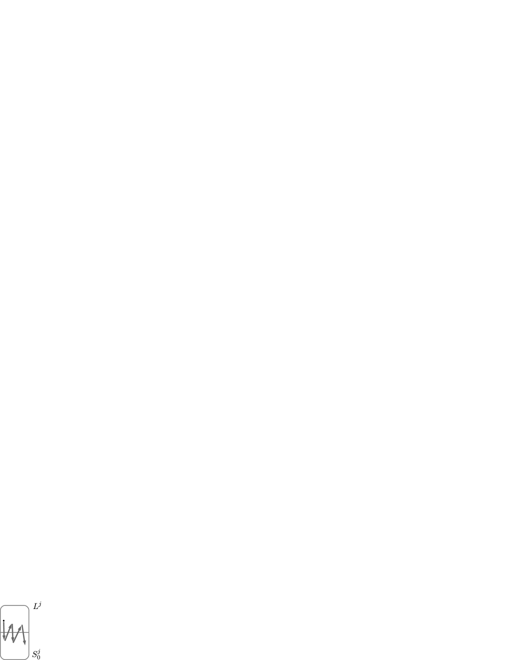
(a) In case $x$ is mapped to $L^{j}$ we can embed the tree $T(\downarrow x)$ greedily in $G[L^{j},S^{j}_{0}]$.

(b) In case $x$ is mapped to $v\in S^{j}$ (but not necessarily in $S^{j}_{0}$) we first embed all its children to $L^{j}$. To this end we make use of Condition $(ii)$. The rest of the embedding goes in $G[L^{j},S^{j}_{0}]$.

Figure 7: Embedding the tree $T(\downarrow x)$ in Lemma 7.11. The placement of $x$ is denoted by a black dot. The embedding the proceeds following the arrows.

The assignment finished, for every $x\in X$ with $j_{x}\neq i$ we map $x$ to $\mathrm{N}(v_{x})\cap(L^{j_{x}}\cup S^{j_{x}})$. This is possible thanks to Condition $(i)$. Having mapped all $X_{\neq i}=\{y\in X\>:\>j_{y}\neq i\}$, we embed $\{\mathrm{Ch}(x),x\in X_{\neq i}\}$ in $L^{j_{x}}\cup S^{j_{x}}_{0}$ (see Figure 7). Even if $x$ is mapped to $S^{j_{x}}$, the at most $\gamma(k+1)$ children of $x$ (cf. definition of $W_{1}^{**}$) can be embedded thanks to Condition $(ii)$ and the definition of $S^{j}$. Having embedded all the vertices $\bigcup_{x\in X_{\neq i}}\mathrm{Ch}(x)$, we continue as follows. For each $x\in X_{\neq i}$ we embed the rest of $T(\downarrow x)$ greedily in $L^{j_{x}}\cup S^{j_{x}}_{0}$, which is possible by (7.28). We are finished with embedding $T$ in the case that $j_{x}\neq i$ for all $x\in X$. Thus, assume that

$$j_{x}=i\text{ for some $x\in X$\;.}$$ (7.29)

Suppose that $\sum_{y\in X\>:\>j_{y}=j}v(T(\downarrow y))>k/(5m)-2\gamma k$ for some $j\neq i$. Set $\mathcal{D}=\{T(\downarrow y)\>:\>j_{y}=j\}$.

Claim 7.11.4.

We have $|U_{1}\cap V(\mathcal{D})|\geq 500\gamma k$.

Proof.

First, consider the case that the total order of small components of $\mathcal{D}$, defined as with at most $10$ vertices, is at least $|V(\mathcal{D})|/2$. In each such component, there is at least one vertex of $W_{1}^{***}\subseteq U_{1}$. Hence $|U_{1}\cap V(\mathcal{D})|\geq\frac{1}{10}\cdot\frac{|V(\mathcal{D})|}{2}\geq\frac{k}{200m}>500\gamma k$.

Next, consider the case that the total order of large components of $\mathcal{D}$ (those having more than 10 vertices) is more than $|V(\mathcal{D})|/2$. Let $\mathcal{D}_{1}$ be those large components $D\in\mathcal{D}$ with $|U_{2}\cap V(D)|<10|U_{1}\cap V(D)|$, and let $\mathcal{D}_{2}$ be those large components $D\in\mathcal{D}$ with $|U_{2}\cap V(D)|\geq 10|U_{1}\cap V(D)|$. Consider the tree $T^{\prime\prime}=T-\mathcal{D}_{2}$, and its colour classes $T^{\prime\prime}_{\oplus}$ and $T^{\prime\prime}_{\ominus}$. Let $R$ be the roots of the trees in $\mathcal{D}_{2}$. We have $|R|\leq|V(\mathcal{D}_{2})|/10$. Set the partition $V(T)=U_{1}^{\prime}\dot{\cup}U_{2}^{\prime}$, where $U_{2}^{\prime}=T^{\prime\prime}_{\oplus}\cup(U_{2}\cap V(\mathcal{D}_{2}))\setminus R$ and $U_{1}^{\prime}=V(T)\setminus U_{2}^{\prime}=T^{\prime\prime}_{\ominus}\cup(U_{1}\cap V(\mathcal{D}_{2}))\cup R$. Observe that $U_{2}^{\prime}$ is an independent set. As $\mathrm{disc}(T)<2\gamma k$, we have

$$2\gamma k>|U_{2}^{\prime}|-|U_{1}^{\prime}|\geq|U_{2}\cap V(\mathcal{D}_{2})|-|U_{1}\cap V(\mathcal{D}_{2})|-2|R|\geq(\tfrac{9}{11}-\tfrac{1}{5})|V(\mathcal{D}_{2})|\;.$$

We conclude that $|V(\mathcal{D}_{2})|<4\gamma k$. In particular, we have $|V(\mathcal{D}_{1})|\geq|V(\mathcal{D})|/4$. Then

$$|U_{1}\cap V(\mathcal{D})|\geq|U_{1}\cap V(\mathcal{D}_{1})|\geq\tfrac{1}{11}\cdot\tfrac{|V(\mathcal{D})|}{4}>500\gamma k\;,$$

as needed. ∎

Recall that we have embedded the entire tree $T$ except the set $M=\bigcup_{x\in X\setminus X_{\neq i}}V(T(\downarrow x))$. Let $Q\subseteq U_{2}\cap M$ be a set of size $\max\{400\gamma k,|U_{2}\cap M|\}$. To finish the embedding of $T$, we embed greedily the vertices of $Q\cup(U_{1}\cap M)$ in $L^{i}$ and the vertices of $(U_{2}\cap M)\setminus Q$ in $S^{i}_{0}$. Prior to this embedding, by Claim 7.11.4, at least $500\gamma k$ vertices of $U_{1}$ had been embedded outside of $L^{i}$. Thus, the minimum-degree conditions (7.1) guarantee that such a greedy embedding indeed exists.

Thus, it remains to consider that $\sum_{y\in X\>:\>j_{y}=j}v(T(\downarrow y))\leq k/(5m)-2\gamma k$ for all $j\neq i$. At the same time, we had not been able to satisfy Condition $(i)$ for any $j\not=i$ for the vertex $x$ from (7.29). Then $\deg(v_{x},\bigcup_{j\neq i}(L^{j}\cup S^{j}))\leq|\{y\in X\>:\>j_{y}\neq i\}|$.

At least

$$(k+1)/2-|L^{i}|\geq|U_{1}|-|L^{i}|$$ (7.30)

vertices of $U_{1}$ were embedded outside $L^{i}$. Indeed, at least $\deg(v_{x},\bigcup_{j\neq i}(L^{j}\cup S^{j}))$ vertices $x\in X$ were assigned some $j_{x}\neq i$. Each corresponding tree $T(\downarrow x)$ contains at least one child of $x$, belonging to $W_{1}^{***}\subseteq U_{1}$, which was thus embedded outside $L^{i}$. Using (7.12), we get (7.30).

It remains to embed the trees $\{T(\downarrow x)\>:\>x\in X\setminus X_{\neq i}\}$. We first embed all the trees $T(\downarrow x)\setminus(W_{1}^{***}\cup W_{2})$, $x\in X\setminus X_{\neq i}$. The extension to $W_{1}^{***}\cup W_{2}$ will be done at the very end.

Set $W_{X}=W_{1}^{***}\cap\left(\bigcup_{x\in X\setminus X_{\neq i}}V(T(\downarrow x))\right)$ and $W_{Y}=W_{1}^{***}\cap\left(\bigcup_{x\in X_{\neq i}}V(T(\downarrow x))\right)$.

Claim 7.11.5.

We have $|W_{X}\cup W_{Y}|\geq 1.9\gamma k$.

Proof.

Let $\tilde{W}$ be all vertices in $W_{1}^{***}\cap V(\tilde{T})\subseteq U_{1}$ whose parent lies in $U_{2}$. For $y\in\tilde{W}$, the independence of $U_{2}$ implies that $\mathrm{Par}(\mathrm{Par}(y))\in U_{1}$. Thus by the definition of $X$, we have that $\mathrm{Par}(y)\in X$ and thus $y\in W_{1}^{***}\cap\left(\bigcup_{x\in X}V(T(\downarrow x))\right)=W_{X}\cup W_{Y}$. Hence, $\tilde{W}\subseteq W_{X}\cup W_{Y}$.

The semi-independent partition

$$\big{(}U_{1}\setminus((W_{1}^{***}\cap V(\tilde{T}))\setminus\tilde{W})\>,\>U_{2}\cup((W_{1}^{***}\cap V(\tilde{T}))\setminus\tilde{W})\big{)}$$

has gap

$$\left(|U_{2}|+|W_{1}^{***}\cap V(\tilde{T})|-|\tilde{W}|\right)-\left(|U_{1}|+|\tilde{W}|-|W_{1}^{***}\cap V(\tilde{T})|\right)$$

$$\geq\left(|W_{1}^{***}\cap V(\tilde{T})|-|\tilde{W}|\right)-\left(|\tilde{W}|-|W_{1}^{***}\cap V(\tilde{T})|\right)\geq 2\cdot 2.9\gamma k-2|\tilde{W}|\;.$$

Since $\mathrm{disc}(T)<2\gamma k$, we get $|\tilde{W}|\geq 1.9\gamma k$. ∎

Set $N=\bigcup_{x\in X_{\neq i}}V(T(\downarrow x))$. By Claim 7.11.5, we have that $|W_{Y}|\geq 0.75\gamma k$, or $|W_{X}|\geq 0.75\gamma k$. Hence,

$$|U_{1}\setminus(W_{X}\cup N)|\leq\frac{k+1}{2}-0.75\gamma k\overset{\mbox{\tiny{\eqref{eq:Am}}}}{\leq}|L^{i}|-\frac{\gamma k}{2}\;.$$ (7.31)

For a fixed $x\in X\setminus X_{\neq i}$, we proceed embedding $T(\downarrow x)\setminus W_{X}$ greedily in $G[L^{i}\cup S^{i}_{0}]$, using $L^{i}$ to host $(U_{1}\cap V(T(\downarrow x)))\setminus W_{X}$, and $S^{i}_{0}$ to host $(U_{2}\cap V(T(\downarrow x)))\setminus W_{2}$. By (7.31), (7.1), and the definition of $S^{i}_{0}$, we have $\deg(v_{x},L^{i})\geq|L^{i}|-\gamma k/2$ and $\delta(S^{i}_{0},L^{i})\geq|L^{i}|-\gamma k/2$ is sufficient to accommodate the vertices from $U_{1}\setminus(W_{X}\cup N)$ in $L^{i}$. As for the vertices that need to be mapped to $S^{i}_{0}$, recall that the fact that $(U_{1},U_{2})$ is $8\gamma k$-ideal yields $|W_{2}|\geq 8\gamma k$. Together with the fact that we are considering the deficient case, we get that at most

$$|U_{2}\setminus W_{2}|\leq(\frac{k}{2}+\gamma k)-8\gamma k\leq|S^{i}_{0}|-7\gamma k$$

vertices are mapped to $S^{i}_{0}$. Hence, the minimum degree of vertices of $L^{i}$ to $S^{i}_{0}$ is sufficient for a greedy embedding.

The next stage is to embed the vertices of $W_{X}$. Let $L^{*}\subseteq L^{i}$ be the set of unused vertices. We consider a bipartite graph $H$ whose two colour classes are $L^{*}$ and $\mathrm{Par}(W_{X})$. A pair $vx$, $v\in L^{*}$, $x\in\mathrm{Par}(W_{X})$ forms an edge in $H$ if $x$ was mapped to a vertex that is adjacent to $v$ in $G$. By the definition of $S^{i}_{0}$, and by (7.1), we have $\delta_{H}(\mathrm{Par}(W_{X}),L^{*})\geq|L^{*}|-\gamma k/2$, and $\delta_{H}(L^{*},\mathrm{Par}(W_{X})\geq|\mathrm{Par}(W_{X})|-\gamma k/2=|W_{X}|-\gamma k/2$. We conclude that $H$ has no vertex cover of size less than $\min\{|W_{X}|,|L^{*}|\}$. As we did not embed any vertex from $W_{X}$ yet, and by (7.30) we mapped to $L^{i}$ at most $|U_{1}|-(|U_{1}|-|L^{i}|)-|W_{X}|=|L^{i}|-|W_{X}|$ vertices, we get $|L^{*}|\geq|W_{X}|$ and thus the minimum vertex cover has size at least $|W_{X}|$. By König’s Theorem, there exists a matching covering $\mathrm{Par}(W_{X})$ in $H$. This matching tells us how to embed $W_{X}$. In the last step, we embed $W_{2}$. This can be done greedily as $\mathrm{Par}(W_{2})$ were mapped to $L$.

The case $|W_{1}^{***}\setminus V(\tilde{T})|\geq 2.9\gamma k$ is treated similarly, the difference being that this time we start with $X=\{x\in\mathrm{Par}(W_{1}^{***}\setminus V(\tilde{T}))\>:\>\mathrm{Par}(x)\in U_{1}\}$. ∎

Appendix A Proofs of some auxiliary facts

Proofs of several auxiliary statements were omitted in the main body of the paper. Here we give these proofs.

A.1 Proof of Lemma 3.8

For the proof we need the following two statements. The first one is a simple corollary of Hall’s Matching Theorem.

Lemma A.1.

Let $K=(W_{1},W_{2};J)$ be a bipartite graph such that $\delta(K)\geq\tfrac{|W_{1}|}{2}$ and $|W_{1}|\leq|W_{2}|$. Then $K$ contains a matching covering $W_{1}$.

Let $\ell$ be the number of leaves of $T$. Recall that $\ell<\alpha k$. Fact 3.2 gives that $\mathrm{disc}(F)<\alpha k$. In particular the lower bounds given in Properties $(v)$ and $(vi)$ of the lemma, combined with the upper bound in Property $(iv)$ yield $|A|,|B|\geq\frac{4k}{10}$.

We write $r=|B_{\mathrm{d}}|$, and $\mathcal{Q}=\{P_{1},\ldots,P_{r}\}$. Root $T$ at an arbitrary vertex $v\in T_{\ominus}$. An $c$-induced path $a_{1}\ldots a_{c+1}\subseteq T$ is a path whose internal vertices have degree two in $T$. Take a maximum family $\mathcal{F}$ of vertex-disjoint 7-induced paths in $T$. We show that $|V(\mathcal{F})|\geq k-19\ell$.

Let $D_{3}=\{u\in V(T)\>:\>\deg_{T}(u)\geq 3\}$ and $D_{i}=\{u\in V(T)\>:\>\deg_{T}(u)=i\}$ for $i=1,2$. By Fact 5.4, we have $|D_{3}|<\ell$ (and $|D_{2}|\geq k-2\ell$). From

$$2k=\sum_{u\in V(T)}\deg(u)=|D_{1}|+2|D_{2}|+\sum_{u\in D_{3}}\deg(u)\geq 2k-3\ell+\sum_{u\in D_{3}}\deg(u)\;,$$

we deduce that there are at most $3\ell+1$ maximal (w. r. t. inclusion) paths formed by vertices of degree $2$ or $1$ not containing the root $v$. On each such maximal path, at most $7$ vertices are not covered by $\mathcal{F}$. Thus the total number of vertices uncovered by $\mathcal{F}$ is at most $7(3\ell+1)+|D_{3}|+|\{v\}|\leq 26\ell$. The order $\preceq_{v}$ naturally extends to an order on the paths of $\mathcal{F}$. For a family $\mathcal{F}^{\prime}\subseteq\mathcal{F}$ we write $T(\downarrow\mathcal{F}^{\prime})$ to denote all the vertices of $V(\mathcal{F}^{\prime})$, and all vertices that are below some vertex of $V(\mathcal{F}^{\prime})$, i.e.,

$$T(\downarrow\mathcal{F}^{\prime})=\bigcup_{u\in V(\mathcal{F}^{\prime})}V(T(\downarrow u))\;\mbox{.}$$

There is a family $\mathcal{R}\subseteq\mathcal{F}$ satisfying the three properties below.

• $|\mathcal{R}|\leq|\mathcal{E}|+|\mathcal{M}|$.

• $|T(\downarrow\mathcal{R})|<34\alpha k$, and $4(|\mathcal{E}|+|\mathcal{M}|)\leq\min\{|T_{\oplus}\cap T(\downarrow\mathcal{R})|,|T_{\ominus}\cap T(\downarrow\mathcal{R})|\}$.

• $\mathcal{R}$ is a $\preceq_{v}$-antichain.

We describe a procedure how to obtain such a family $\mathcal{R}$. By an inductive construction, we first find an auxiliary family $\mathcal{R}^{\prime}$, starting with $\mathcal{R}^{\prime}=\emptyset$. While $|\mathcal{R}^{\prime}|<|\mathcal{E}|+|\mathcal{M}|$ we take a $\preceq_{v}$-minimal path in $\mathcal{F}$ which is not included in $\mathcal{R}^{\prime}$ and add it to $\mathcal{R}^{\prime}$. From the bound $|V(T)\setminus V(\mathcal{F})|\leq 26\ell$, in each step we have that $|T(\downarrow\mathcal{R}^{\prime})|<8|\mathcal{R}^{\prime}|+26\alpha k$, and obviously $4|\mathcal{R}^{\prime}|\leq\min\{|T_{\oplus}\cap T(\downarrow\mathcal{R}^{\prime})|,|T_{\ominus}\cap T(\downarrow\mathcal{R}^{\prime})|\}$. Let $\mathcal{R}$ be the $\preceq_{v}$-maximal elements of $\mathcal{R}^{\prime}$. Hence $|T(\downarrow\mathcal{R})|=|T(\downarrow\mathcal{R}^{\prime})|$. The properties (P1), (P2), and (P3) are satisfied.

Set $d=5\alpha k$. Take a family $\mathcal{X}=\{X_{1},\ldots,X_{d}\}$ of $d$ 5-induced vertex-disjoint $T_{\oplus}-T_{\ominus}-T_{\oplus}-T_{\ominus}-T_{\oplus}$ paths that avoid $\{v\}\cup T(\downarrow\mathcal{R})$. For each path $R\in\mathcal{R}$ we write $a_{R}$ to denote its $\preceq_{v}$-maximum vertex in $T_{\ominus}$, and set $b_{R}=\mathrm{Ch}(a_{R})$, $c_{R}=\mathrm{Ch}(b_{R})$, and $d_{R}=\mathrm{Ch}(c_{R})$. We set $U=A\cap(V(\mathcal{E})\cup V(\mathcal{M}))$ and $Q=A\cap V(\mathcal{Q})$.

We now describe the embedding $\psi$ of $T$. We do not have to embed those leaves whose parents are embedded in $A$ until the very end. Indeed, such a partial embedding easily extends to an embedding of $T$ using Property $(ii)$ of the lemma. We map the root $v$ to an arbitrary vertex in $A\setminus(U\cup Q)$. We continue embedding $T$ greedily, mapping vertices from $T_{\ominus}$ to $A\setminus(U\cup Q)$ and internal vertices of $T_{\oplus}$ to $B_{\mathrm{a}}$. However, there are two exceptions in the greedy procedure:

• If we are about to map a vertex $b_{R}$ (for some $R\in\mathcal{R}$), we skip its embedding, as well as the embedding of $T(\downarrow b_{R})$.

• If we are about to map a vertex $x_{2}$ which was part of some path $x_{1}x_{2}x_{3}x_{4}x_{5}\in\mathcal{X}$, we skip its embedding, as well as the embedding of the vertices $x_{3}$ and $x_{4}$. We continue with mapping $x_{5}$ to $B_{\mathrm{a}}$.

Observe that we are able to finish the greedy part of the embedding since the two “skipping rules” guarantee that both in $A$ and in $B$ at least $d>\alpha k$ vertices of $T$ remain unembedded.

In the next step, we build missing connections in the graph $H$ caused by the skipping rules. We construct an auxiliary bipartite graph $K_{1}=(O_{\mathrm{a}},O_{\mathrm{b}};E_{1})$. We arbitrarily pair up $2(d-r)$ vertices of $A\setminus(U\cup Q)$ unused by $\psi$ into pairs $\mu_{1}=\{a_{1}^{1},a_{1}^{2}\},\ldots,\mu_{d-r}=\{a_{d-r}^{1},a_{d-r}^{2}\}$. The remaining $r$ pairs are formed by endvertices of the paths in $\mathcal{Q}$. We set $\mu_{i+d-r}=A\cap V(P_{i})$. Vertices of the color class $O_{\mathrm{b}}$ are formed by the pairs $\mu_{i}$ ($i\in[d]$). Vertices of the color class $O_{\mathrm{a}}$ are formed by the paths in $\mathcal{X}$. A path $x_{1}x_{2}x_{3}x_{4}x_{5}\in\mathcal{X}$ is adjacent in $K_{1}$ to a pair $\mu_{i}$ if and only if there exists a perfect matching in the graph $H[\{\psi(x_{1}),\psi(x_{5})\},\mu_{i}]$. Since $|O_{\mathrm{a}}|=|O_{\mathrm{b}}|$ and $\delta(K_{1})\geq|O_{\mathrm{a}}|-2\alpha k\geq\tfrac{|O_{\mathrm{a}}|}{2}$, there exists, by Lemma A.1, a perfect matching $M_{1}$ in $K_{1}$. The matching $M_{1}$ tells us where to map the vertices $x_{2}$ and $x_{4}$ of each path $x_{1}x_{2}x_{3}x_{4}x_{5}\in\mathcal{X}$. We extend $\psi$ accordingly on the vertices $\bigcup_{x_{1}x_{2}x_{3}x_{4}x_{5}\in\mathcal{X}}\{x_{2},x_{4}\}$. If a path $x_{1}x_{2}x_{3}x_{4}x_{5}\in\mathcal{X}$ was matched with $\mu_{i+d-r}$ (for some $i\in[r]$) in $K_{1}$, we map $x_{3}$ to the middle vertex of the path $P_{i}$. We write $\mathcal{X}^{\prime}$ for those paths $x_{1}x_{2}x_{3}x_{4}x_{5}\in\mathcal{X}$ whose vertex $x_{3}$ was not yet mapped. It holds $|\mathcal{X}^{\prime}|\geq 4\alpha k$.

Let $\xi:\mathcal{R}\rightarrow U$ be an arbitrary injective mapping. We construct another bipartite graph $K_{2}=(J_{\mathrm{a}},J_{\mathrm{b}};E_{2})$. Vertices of the color class $J_{\mathrm{a}}$ are elements of $\mathcal{R}\cup\mathcal{X}^{\prime}$ and vertices of the color class $J_{\mathrm{b}}$ are vertices of $B_{\mathrm{a}}$ unused by $\psi$.

Claim A.1.1.

We have $|J_{\mathrm{a}}|\leq|J_{\mathrm{b}}|$.

Proof.

Let $W$ be the set of leaves of $T_{\oplus}\setminus V(\mathcal{R})$. Remember that the set $W$ is mapped only at the very end of the embedding procedure. Further, for any path $x_{1}\ldots x_{5}\in\mathcal{X}\setminus\mathcal{X}^{\prime}$, the vertex $x_{3}\in T_{\oplus}$ has been mapped to $B_{\mathrm{d}}$, which is disjoint from $B_{\mathrm{a}}$. Next for each path $x_{1}\ldots x_{5}\in\mathcal{X}^{\prime}$, the vertex $x_{3}\in T_{\oplus}$ has not been embedded, yet. Each path in $\mathcal{R}$ has at most one vertex in $T_{\oplus}$ that has already been embedded. Therefore we have

$$|J_{\mathrm{b}}| \geq|B|-\big{(}|T_{\oplus}|-|W|-|X\setminus X^{\prime}|-|X^{\prime}|-(|T_{\oplus}\cap V(\downarrow\mathcal{R})|-|\mathcal{R}|)\big{)}$$

$$\geq|B|-|T_{\oplus}|+|W|+|X|+3(|\mathcal{E}|+|\mathcal{M}|)$$

$$\geq|W|+|X|+2|\mathcal{R}|-1\geq|J_{\mathrm{a}}|+|W|+|R|-1\geq|J_{\mathrm{a}}|\>,$$

where the last inequality follows from the fact that if $\mathcal{R}=\emptyset$ then $W\neq\emptyset$ by FactFact 3.2. ∎

A path $R\in\mathcal{R}$ is adjacent in $K_{1}$ with a vertex $b\in J_{\mathrm{b}}$ if and only if $b\psi(a_{R})\in E(H)$ and $b\xi(R)\in E(H)$. A path $x_{1}x_{2}x_{3}x_{4}x_{5}\in\mathcal{X}^{\prime}$ is adjacent to a vertex $b\in J_{\mathrm{b}}$ if and only if $b\psi(x_{2})\in E(H)$ and $b\psi(x_{4})\in E(H)$. Indeed, $\delta(K_{1})\geq|J_{\mathrm{a}}|-2\gamma k>\tfrac{|J_{\mathrm{a}}|}{2}$, and $|J_{\mathrm{a}}|\leq|J_{\mathrm{b}}|$. By Lemma A.1, there exists a matching $M_{2}$ in $K_{2}$ covering $J_{\mathrm{a}}$. Such a matching tells us where to map unembedded vertices $x_{3}$ (in the case of a path $x_{1}x_{2}x_{3}x_{4}x_{5}\in\mathcal{X}^{\prime}$) and vertices $b_{R}$ (in the case of a path $R\in\mathcal{R}$). For a path $R\in\mathcal{R}$ we finish embedding the part of the tree $T(\downarrow c_{R})$, extending the mapping $\psi$. If $\psi(c_{R})\in V(\mathcal{E})$ we just use the corresponding connecting edge of $\mathcal{E}$ to map $d_{R}$ to $H_{\kappa}$ (for some $\kappa\in I$) and continue embedding $T(\downarrow d_{R})$ greedily in $H_{\kappa}$. If $\psi(c_{R})\in V(\mathcal{M})$ we map $d_{R}$ to the middle vertex of the corresponding connecting path $\mathcal{M}$ and embed the rest of $T(\downarrow d_{R})$ greedily in $H_{\kappa}$ (for some $\kappa\in I$).

A.2 Omitted proofs from Section 5

Proof of Fact 5.9 $(i)$.

Let $\tilde{X}\subseteq X$ be the set of vertices that are not typical w. r. t. $\bigcup_{i=1}^{\ell}W_{i}$, i.e., for every $v\in\tilde{X}$ we have $\deg(v,\bigcup_{i=1}^{\ell}W_{i})<\sum_{i=1}^{\ell}(d(X,Y_{i})-\varepsilon)|W_{i}|$. Thus $e(\tilde{X},\bigcup_{i=1}^{\ell}W_{i})<|\tilde{X}|\cdot\sum_{i=1}^{\ell}(d(X,Y_{i})-\varepsilon)|W_{i}|$. Hence, there is an index $i\in[\ell]$ such that $d(\tilde{X},W_{i})<d(X,Y_{i})-\varepsilon$. As $W_{i}$ is significant and $(X,Y_{i})$ is $\varepsilon$-regular, we get that $|\tilde{X}|\leq\varepsilon|X|$. ∎

Proof of Lemma 5.12.

Without loss of generality assume that $|P^{\prime}|\geq\Delta$. Let us fix an arbitrary set $S_{P}\subseteq P$ with $|S_{P}|=\Delta$ and another set $S_{Q}\subseteq Q$ with $|S_{Q}|=\Delta$. The sets $S_{P}$ and $S_{Q}$ are significant. Choose a vertex $v\in P^{\prime}$ which is typical w. r. t. $S_{Q}$. There are at least $|P^{\prime}|-\varepsilon s\geq 1$ such vertices. Set $\phi(r)=v$.

We inductively extend the embedding $\phi$, so that every vertex of $t$ that is mapped to $S_{P}$ is typical w. r. t. $S_{Q}$, and so that every vertex that is mapped to $S_{Q}$ is typical w. r. t. $S_{P}$. We illustrate the inductive step by describing how to embed the neighborhood of a vertex $u$ that was already mapped to $P$. The case that $\phi(u)\in Q$ is analogous. Let $N\subseteq\mathrm{N}(u)$ be the yet unembedded neighbors of $u$. The vertex $\phi(u)$ has at least $(d-2\varepsilon)\Delta\geq\varepsilon s+v(t)$ neighbors in $S_{Q}$. At least $|N|$ of them are typical w. r. t. $S_{P}$ and are not yet used by $\phi$. We map $N$ to these vertices.

For the moreover part, we only need to observe that if $|P^{\prime}|\geq\Delta$, there is at least one vertex in $P^{\prime}$ which is typical w. r. t. $S_{Q}$. We map the root $r$ to this vertex. The second condition of the moreover part is analogous. ∎

For the proof of Lemma 5.13, we need to embed the shrubs of a given tree in an efficient way. To this end, we try to fill the clusters of a regular pair in a balanced way. The following definition of packedness formalizes this. Let $X,Y,Z$ be three disjoint sets of vertices of a graph $G$. We say that $U\subseteq X\cup Y$ is $(\lambda,\tau)$-packed with respect to the head set $Z$ and the embedding sets $X$ and $Y$, if

$$\min\{|X\cap U|,|Y\cap U|\} \geq\min\{\mathrm{d\overline{eg}}_{\mathbf{H}}(Z,X),\mathrm{d\overline{eg}}_{\mathbf{H}}(Z,Y)\}-\lambda,\mbox{or}$$ (A.1)

$$\left||X\cap U|-|Y\cap U|\right| \leq\tau$$ (A.2)

Proof of Lemma 5.13.

Assume that $\mathbf{H}$ has $N$ clusters. Let $\tilde{X}\subseteq X^{\prime}$ be the set of vertices that are typical w. r. t. all but at most $\sqrt{\varepsilon}N$ sets $C\cap V^{X}$, $C\in V(M)$, w. r. t. all but at most $\sqrt{\varepsilon}N$ clusters $Z\in\mathcal{Z}$, and w. r. t. the cluster $Y$. Let $\tilde{Y}\subseteq Y^{\prime}$ be the set of vertices that are typical w. r. t. all but at most $\sqrt{\varepsilon}N$ sets $C\cap V^{Y}$, $C\in V(M)$ and w. r. t. the cluster $X$. Let $\tilde{Z}\subseteq\bigcup\mathcal{Z}$ be the set of vertices (viewed as vertices of individual clusters of $\mathcal{Z}$) that are typical w. r. t. all but at most $\sqrt{\varepsilon}N$ sets $C\cap V^{\mathcal{Z}}$, $C\in V(M)$ and w. r. t. the cluster $X$. Observe that by Fact 5.9, $|X^{\prime}\setminus\tilde{X}|\leq 3\sqrt{\varepsilon}s$, $|Y^{\prime}\setminus\tilde{Y}|\leq 2\sqrt{\varepsilon}s$, and for every $Z\in\mathcal{Z}$,

$$|Z\setminus\tilde{Z}|\leq 2\sqrt{\varepsilon}s\;.$$ (A.3)

Let $Q_{X}$ be the set of vertices (viewed as vertices of individual clusters of $V(\mathbf{H})$) typical w. r. t. $\tilde{X}$. We define analogously $Q_{Y}$. For each $v\in\tilde{X}\cup\tilde{Y}$, let

$$M_{v} =\{CD\in M\>:\>v\textrm{ is typical w.~{}r.~{}t.\ both }C\cap V^{X}\textrm{ and }D\cap V^{X}\}\quad\mbox{if $v\in\tilde{X}$}\;,$$

$$M_{v} =\{CD\in M\>:\>v\textrm{ is typical w.~{}r.~{}t.\ both }C\cap V^{Y}\textrm{ and }D\cap V^{Y}\}\quad\mbox{if $v\in\tilde{Y}$}\;.$$

For each cluster $C\in V(M)$ we have by Fact 5.9,

$$|C\setminus Q_{X}|,|C\setminus Q_{Y}| \leq\varepsilon s\;,\quad\mbox{ and }$$ (A.4)

$$|M_{v}| \geq|M|-2\sqrt{\varepsilon}N\;.$$ (A.5)

The embedding of $F$ is divided into $w$ steps, where $w=|W_{X}\cup W_{Y}|$. We label the vertices of $W_{X}\cup W_{Y}$ as $x_{1},\ldots,x_{w}$, indexing from an arbitrary fixed root $R\in W_{X}\cup W_{Y}$ downwards, i.e., in such way that $j_{1}\leq j_{2}$ whenever $x_{j_{1}}\succeq_{R}x_{j_{2}}$. We denote by $\varphi$ the partial embedding of $F$. For a set $U\subseteq V(F)$, $\varphi(U)$ refers to the image of the already embedded part of $U$ at that moment. In step $i\geq 1$, we embed the tree

$$F_{i}=F\Big{[}\{x_{i}\}\cup\bigcup_{\ell\in[c_{i}]}V(t_{i}^{\ell})\Big{]}\;\mbox{,}$$

where $t_{i}^{1},\ldots,t_{i}^{c_{i}}$ are the components $t\in\mathcal{D}_{X}\cup\mathcal{D}_{Y}$ such that $\mathrm{Ch}(x_{i})\cap V(t)\not=\emptyset$. Set $V_{i}^{\ell}=\bigcup_{j<i}V(F_{j})\cup\bigcup_{j<\ell}V(t_{i}^{j})$, and $U_{i}^{\ell}=\varphi(V_{i}^{\ell})$. We call the embedding $\varphi$ equable at step $i$ and substep $\ell$, if for each $CD\in M$, we have $||U_{i}^{\ell}\cap V^{\mathcal{Z}}\cap C|-|U_{i}^{\ell}\cap V^{\mathcal{Z}}\cap D||\leq\tau$. During the embedding procedure, we use an auxiliary set $\mathcal{Z}^{\prime}\subseteq\mathcal{Z}$ of “active” clusters in $\mathcal{Z}$.

For $i=1$, set $N_{i}=\tilde{X}\cup\tilde{Y}$ and $\mathcal{Z}^{\prime}=\mathcal{Z}$. For $i>1$, let $p_{i}=\mathrm{Par}(x_{i})$ and set $N_{i}=\mathrm{N}_{H}(\varphi(p_{i}))\cap(\tilde{X}\cup\tilde{Y})$. During the embedding process we will keep the following three properties in every step $i\in[w]$, and every substep $j\in[c_{i}]$.

• For each $CD\in M$, the set $U_{i}^{j}\cap V^{X}\cap(C\cup D)$ is $(\tfrac{8\varepsilon s}{d},\tau)$-packed w. r. t. the head set $X$ and the set $U_{i}^{j}\cap V^{Y}\cap(C\cup D)$ is $(\tfrac{8\varepsilon s}{d},\tau)$-packed w. r. t. the head set $Y$.

• $|N_{i}\cap X|\geq|W_{X}|$ and $|N_{i}\cap Y|\geq|W_{Y}|$.

• $\varphi(W_{X})\subseteq\tilde{X}$, $\varphi(W_{Y})\subseteq\tilde{Y}$, $\varphi(\mathcal{D}_{Y})\subseteq V^{Y}$, $\varphi(\mathcal{D}_{1})\subseteq V^{X}\setminus V(M_{X})$, $\varphi(\mathcal{D}_{2})\subseteq V^{X}\cap V(M_{X})$, $\varphi(\mathcal{D}_{3}\setminus\mathrm{N}_{F}(W_{X}))\subseteq V^{\mathcal{Z}}$, and $\varphi(\mathcal{D}_{3}\cap\mathrm{N}_{F}(W_{X}))\subseteq\bigcup\mathcal{Z}$.

• Either the embedding $\varphi$ is equable and $\mathcal{Z}^{\prime}=\mathcal{Z}$, or for every $CD\in M$ and every $Z\in\mathcal{Z}^{\prime}$ we have

  $$\min\{\mathrm{d\overline{eg}}_{\mathbf{H}}(Z,C\cap V^{\mathcal{Z}}),\mathrm{d\overline{eg}}_{\mathbf{H}}(Z,D\cap V^{\mathcal{Z}})\}\leq\min\{|(C\cap\varphi(\mathcal{D}_{3})|,|(D\cap\varphi(\mathcal{D}_{3})|\}+\frac{8\varepsilon s}{d}\;,$$

  and $\mathrm{d\overline{eg}}_{\mathbf{H}}(X,\bigcup\mathcal{Z}^{\prime})\geq|(V(\mathcal{D}_{3})\cap\mathrm{N}_{F}(W_{X}))\setminus V_{i}^{j}|+|U_{i}^{j}\cap\bigcup\mathcal{Z}^{\prime}|+\frac{\xi n}{2}\;.$

For $i=1$ and $j=1$, (I1), (I3), and (I4) hold trivially. Further, $\max\{|W_{X}|,|W_{Y}|\}\leq\tfrac{12k}{\tau}\ll\varepsilon s\leq\min\{|\tilde{X}|,|\tilde{Y}|\}$ by Definition 5.2 $(vi)$, yielding (I2).

We now proceed with a general step. We first give two claims which we then make use of for the embedding itself.

Claim A.1.2.

 

1. Suppose that $\mathcal{D}_{Y}\neq\emptyset$. Then for every $v\in\tilde{Y}$, there is an edge $CD\in M_{v}$ such that

   $$\deg(v,(C\cup D)\cap V^{Y})\geq|\varphi(\mathcal{D}_{Y})\cap(C\cup D)|+2\tau+\frac{\xi s}{2}\;.$$

2. Suppose that $\mathcal{D}_{1}\neq\emptyset$. Then for every $v\in\tilde{X}$, there is an edge $CD\in M_{v}\setminus M_{X}$ such that

   $$\deg(v,(C\cup D)\cap V^{X}\cap Q_{X})\geq|\varphi(\mathcal{D}_{1})\cap(C\cup D)|+2\tau+\frac{\xi s}{2}\;.$$

3. Suppose that $\mathcal{D}_{2}\neq\emptyset$. Then for every $v\in\tilde{X}$, there is an edge $CD\in M_{X}\cap M_{v}$ such that

   $$\deg(v,C\cap V^{X}\cap Q_{X})\geq|\varphi(\mathcal{D}_{2})\cap C|+\frac{\xi s}{2}\quad\mbox{and}\quad|D\cap V^{X}|\geq|\varphi(\mathcal{D}_{2})\cap D|+\frac{\xi s}{2}\;.$$ (A.6)

4. Suppose that $\mathcal{D}_{3}\neq\emptyset$. Then for every $v\in\tilde{X}$, there is a cluster $Z\in\mathcal{Z}^{\prime}$ such that

   $$\deg(v,Z\cap\tilde{Z})\geq|\varphi(\mathcal{D}_{3})\cap Z|+\frac{\xi s}{4}\;.$$ (A.7)

Proof.

$(a)$ Using the typicality of $v$, we get

$$\sum_{CD\in M_{v}}\deg(v,(C\cup D)\cap V^{Y})\overset{\mbox{\tiny{\eqref{eq:sizeMv}}}}{\geq}\mathrm{d\overline{eg}}_{\mathbf{H}}(Y,V^{Y})-2\sqrt{\varepsilon}Ns-\varepsilon n\overset{\mbox{\tiny{\ref{emb3-V^Y}}}}{\geq}v(\mathcal{D}_{Y})+\frac{3\xi n}{4}\;,$$

which implies the statement.

The proof of $(b)$ is analogous, using (A.4) and $(iv)$.

$(c)$ By (A.5) and by the typicality of $v$, we have

$$\sum_{C\in V(M_{X}\cap M_{v})\cap\mathrm{N}_{\mathbf{H}}(X)}\deg(v,C\cap V^{X}) \geq\sum_{CD\in M_{X}}\deg(v,(C\cup D)\cap V^{X})-2\sqrt{\varepsilon}Ns$$

$$\geq\mathrm{d\overline{eg}}_{\mathbf{H}}(X,V^{X}\cap\bigcup V(M_{X}))-\varepsilon n-2\sqrt{\varepsilon}Ns$$

$$\overset{\mbox{\tiny{\ref{emb3-MX}}}}{\geq}v(\mathcal{D}_{2})-c^{2}k+\xi n-3\sqrt{\varepsilon}Ns\;.$$

As $\mathcal{D}_{2}$ is $c$-balanced, we get $v(\mathcal{D}_{2})\geq c^{2}k+\sum_{CD\in M_{X}\cap M_{v}}\max\{|\varphi(\mathcal{D}_{2})\cap C|,|\varphi(\mathcal{D}_{2})\cap D|\}$. So, there is an edge $CD\in M_{X}\cap M_{v}$ such that

$$|D\cap V^{X}|\overset{\mbox{\tiny{\ref{emb3-balanced}}}}{\geq}\deg(v,C\cap V^{X})\geq\max\{|\varphi(\mathcal{D}_{2})\cap C|,|\varphi(\mathcal{D}_{2})\cap D|\}+\xi s-3\sqrt{\varepsilon}s\;.$$

Together with (A.4), we get (A.6).

$(d)$ The vertex $v$ is typical w. r. t. all but at most $\sqrt{\varepsilon}N$ clusters $Z\in\mathcal{Z}^{\prime}$.

First assume that $\varphi$ is equable and $\mathcal{Z}^{\prime}=\mathcal{Z}$. We have

$$\deg(v,\tilde{Z}\cap\bigcup\mathcal{Z}^{\prime})\; \overset{\mbox{\tiny{$\mathcal{Z}^{\prime}=\mathcal{Z}$}}}{\geq}\;\deg(v,\bigcup\mathcal{Z})-\left|\bigcup\mathcal{Z}\setminus\tilde{Z}\right|\;\overset{\mbox{\tiny{\eqref{eq:cafedu}}}}{\geq}\;\mathrm{d\overline{eg}}_{\mathbf{H}}(X,\bigcup\mathcal{Z})-\varepsilon n-(1+2)\sqrt{\varepsilon}Ns$$

$$\overset{\mbox{\tiny{\ref{emb3-AZ}}}}{\geq}|V(\mathcal{D}_{3})\cap\mathrm{N}_{F}(W_{X})|+\xi n-4\sqrt{\varepsilon}n\;.$$

As by (I3) only $V(\mathcal{D}_{3})\cap\mathrm{N}_{F}(W_{X})$ is mapped to $\bigcup\mathcal{Z}=\bigcup\mathcal{Z}^{\prime}$, there exists a cluster $Z\in\mathcal{Z}^{\prime}$ satisfying (A.7).

If $\varphi$ is not equable, we get

$$\deg(v,\tilde{Z}\cap\bigcup\mathcal{Z}^{\prime}) \geq\deg(v,\bigcup\mathcal{Z}^{\prime})-\left|\bigcup\mathcal{Z}\setminus\tilde{Z}\right|\geq\mathrm{d\overline{eg}}_{\mathbf{H}}(X,\bigcup\mathcal{Z}^{\prime})-\varepsilon n-(1+2)\sqrt{\varepsilon}Ns$$

$$\overset{\mbox{\tiny{{\bf(I4)}}}}{\geq}|V(\mathcal{D}_{3})\cap\mathrm{N}_{F}(W_{X})\setminus V_{i}^{j}|+|U_{i}^{j}\cap\bigcup\mathcal{Z}^{\prime}|+\xi n/2-4\sqrt{\varepsilon}n\;.$$

As by (I3) only $V(\mathcal{D}_{3})\cap\mathrm{N}_{F}(W_{X})$ is mapped to $\bigcup\mathcal{Z}^{\prime}$, there exists a cluster $Z\in\mathcal{Z}^{\prime}$ satisfying (A.7). ∎

Claim A.1.3.

Suppose that $\mathcal{D}_{3}\neq\emptyset$. Then for every vertex $v\in\tilde{Z}$, there is an edge $CD\in M_{v}$ such that

$$\deg(v,(C\cup D)\cap V^{\mathcal{Z}})\geq|\varphi(\mathcal{D}_{3})\cap(C\cup D)|+2\tau+2\varepsilon s+\frac{\xi s}{2}\;.$$ (A.8)

Proof.

Suppose that $v$ lies in a cluster $Z$. Using the typicality of $v$, we get

$$\sum_{CD\in M_{v}}\deg(v,(C\cup D)\cap V^{\mathcal{Z}})\overset{\mbox{\tiny{\eqref{eq:sizeMv}}}}{\geq}\mathrm{d\overline{eg}}_{\mathbf{H}}(Z,V^{\mathcal{Z}})-4\sqrt{\varepsilon}Ns-\varepsilon n\overset{\mbox{\tiny{\ref{emb3-Z}}}}{\geq}v(\mathcal{D}_{3})+\frac{3\xi n}{4}\;.$$

∎

Assume that we are in step $i\geq 1$ and that we want to embed the forest $F_{i}$. By (I2), we can map $x_{i}$ to an unused vertex in $N_{i}$ (in $N_{i}\cap X$ if $x_{i}\in W_{X}$, and in $N_{i}\cap Y$ if $x_{i}\in W_{Y}$). Observe that $\varphi(x_{i})$ has at least $(d-\varepsilon)s-ds/2-3\sqrt{\varepsilon}s\geq\varepsilon s\geq|W_{X}\cup W_{Y}|$ neighbors in $\tilde{X}$ or in $\tilde{Y}$ (depending whether $\varphi(x_{i})\in\tilde{Y}$ or $\varphi(x_{i})\in\tilde{X}$). This ensures that (I2) still holds. Assume that we are in substep $j\in[c_{i}]$, i.e., we have already embedded the components $t_{i}^{1},\dots,t_{i}^{j-1}$ and that we want to embed the component $t_{i}^{j}$.

• If $t_{i}^{j}\in\mathcal{D}_{Y}$, pick an edge $CD\in M_{\varphi(x_{i})}$ as in Claim A.1.2 $(a)$. We use Lemma 5.12 to embed $t_{i}^{j}$ (where the root of $t_{i}^{j}$ is the neighbor of $x_{i}$) with the following setting.

  $$P^{\prime} =\mathrm{N}_{H}(\varphi(x_{i}))\cap C\cap V^{Y}\setminus U_{i}^{j}\qquad P=C\cap V^{Y}\setminus U_{i}^{j}\subseteq C\;,$$

  $$Q^{\prime} =\mathrm{N}_{H}(\varphi(x_{i}))\cap D\cap V^{Y}\setminus U_{i}^{j}\qquad Q=D\cap V^{Y}\setminus U_{i}^{j}\subseteq D\;,$$

  and $\Delta=\tfrac{4\varepsilon s}{d}$. We have that

  $$\max\{|P^{\prime}|,|Q^{\prime}|\}\geq\frac{1}{2}\deg(\varphi(x_{i}),(C\cup D)\cap V^{Y}\setminus U_{i}^{j})\geq\frac{1}{2}(2\tau+\tfrac{\xi s}{2})\geq\tfrac{4\varepsilon s}{d}\;,$$

  which verifies one of the assumption of Lemma 5.12. We use Lemma 5.12 differently in cases

  $$\min\{|\varphi(\mathcal{D}_{Y})\cap C|,|\varphi(\mathcal{D}_{Y})\cap D|\} <\min\{\mathrm{d\overline{eg}}_{\mathbf{H}}(X,C\cap V^{Y}),\mathrm{d\overline{eg}}_{\mathbf{H}}(X,D\cap V^{Y})\}-\tfrac{8\varepsilon s}{d}\quad{\mbox{and}}$$ (A.9)

  $$\min\{|\varphi(\mathcal{D}_{Y})\cap C|,|\varphi(\mathcal{D}_{Y})\cap D|\} \geq\min\{\mathrm{d\overline{eg}}_{\mathbf{H}}(X,C\cap V^{Y}),\mathrm{d\overline{eg}}_{\mathbf{H}}(X,D\cap V^{Y})\}-\tfrac{8\varepsilon s}{d}$$ (A.10)

  Suppose first that we do not have (A.9). Thus in particular, the packedness of $U_{i}^{j}\cap V^{X}\cap(C\cup D)$ in (I1) has the form of (A.2). Then

  $$\min\{|P^{\prime}|,|Q^{\prime}|\} =\min\{\deg(\varphi(x_{i}),C\cap V^{Y}\setminus U_{i}^{j}),\deg(\varphi(x_{i}),D\cap V^{Y}\setminus U_{i}^{j})\}$$

  $$\overset{\mbox{\tiny{{\bf(I3)}}}}{\geq}\min\{\deg(\varphi(x_{i}),C\cap V^{Y}),\deg(\varphi(x_{i}),D\cap V^{Y})\}-\max\{|\varphi(\mathcal{D}_{Y})\cap C|,|\varphi(\mathcal{D}_{Y})\cap D|\}$$

  $$\overset{\mbox{\tiny{{\bf(I1)}}}}{\geq}\min\{\mathrm{d\overline{eg}}_{\mathbf{H}}(X,C\cap V^{Y}),\mathrm{d\overline{eg}}_{\mathbf{H}}(X,D\cap V^{Y})\}-\varepsilon s$$

  $$~{}~{}~{}~{}~{}-\min\{|\varphi(\mathcal{D}_{Y})\cap C|,|\varphi(\mathcal{D}_{Y})\cap D|\}-\tau$$

  $$\overset{\mbox{\tiny{\eqref{eq:c1E1}}}}{\geq}\tfrac{8\varepsilon s}{d}-\varepsilon s-\tau\geq\tfrac{4\varepsilon s}{d}\;,$$

  which allows us to use the “moreover” part of Lemma 5.12. We can then choose in this case to which set $P^{\prime}$ or $Q^{\prime}$ we map the root of $t_{i}^{j}$. We thus can ensure that $\big{|}|\varphi(\mathcal{D}_{Y})\cap C|-|\varphi(\mathcal{D}_{Y})\cap D|\big{|}\leq\tau$ still holds after embedding $t_{i}^{j}$, yielding (I1).

  Suppose now that (A.9) holds. Then

  $$\min\{|P|,|Q|\} =\min\{|C\cap V^{Y}\setminus U_{i}^{j}|,|D\cap V^{Y}\setminus U_{i}^{j}|\}$$

  $$\geq\max\{\deg(\varphi(x_{i}),C\cap V^{Y}),\deg(\varphi(x_{i}),D\cap V^{Y})\}-\max\{|\varphi(\mathcal{D}_{Y})\cap C|,|\varphi(\mathcal{D}_{Y})\cap D|\}$$

  $$\geq \deg(\varphi(x_{i}),(C\cup D)\cap V^{Y})-|\varphi(\mathcal{D}_{Y})\cap(C\cup D)|$$

  $$-\min\{\deg(\varphi(x_{i}),C\cap V^{Y}),\deg(\varphi(x_{i}),D\cap V^{Y})\}+\min\{|\varphi(\mathcal{D}_{Y})\cap C|,|\varphi(\mathcal{D}_{Y})\cap D|\}$$

  $$\overset{\mbox{\tiny{\eqref{eq:c1E1}}}}{\geq} 2\tau+\tfrac{\xi s}{2}-\tfrac{8\varepsilon s}{d}-\varepsilon s\geq\tfrac{4\varepsilon s}{d}\;,$$

  which indeed allows us to embed $t^{j}_{i}$ using Lemma 5.12 in this case. After the embedding of $t_{i}^{j}$ in this case, (I1) holds trivially.

  In both cases, (I2) holds, as $\mathcal{D}_{Y}$ contains only end-shrubs. The tree $t_{i}^{j}$ was embedded in $(C\cup D)\cap V^{Y}$, ensuring (I3). (I4) is immaterial in this step as nothing was done regarding $V^{\mathcal{Z}}$ or $\mathcal{D}_{3}$.

• If $t_{i}^{j}\in\mathcal{D}_{1}$, pick an edge $CD\in M_{\varphi(x_{i})}\setminus M_{X}$ as in Claim A.1.2 $(b)$. The embedding is done analogously to the case (1), setting

  $$P^{\prime} =\mathrm{N}_{H}(\varphi(x_{i}))\cap C\cap V^{X}\cap Q_{X}\setminus U_{i}^{j}\qquad P=C\cap V^{X}\cap Q_{X}\setminus U_{i}^{j}\subseteq C\;,$$

  $$Q^{\prime} =\mathrm{N}_{H}(\varphi(x_{i}))\cap D\cap V^{X}\cap Q_{X}\setminus U_{i}^{j}\qquad Q=D\cap V^{X}\cap Q_{X}\setminus U_{i}^{j}\subseteq D\;.$$

  As $\varphi(V(t_{i}^{j}))\subseteq Q_{X}$, every vertex in $V(t_{i}^{j})\cap\mathrm{N}_{F}(W_{X})$ is mapped to a vertex that has at least $(d-\varepsilon)|\tilde{X}|\geq|W_{X}|$ neighbours in $\tilde{X}$, ensuring (I2). Conditions (I1) and (I3) are maintained as in case (1). Again, (I4) is maintained automatically.

• If $t_{i}^{j}\in\mathcal{D}_{2}$, we pick an edge $CD\in M_{\varphi(x_{i})}\cap M_{X}$ as in Claim $(c)$. We use Lemma 5.12 with the following setting.

  $$P^{\prime} =\mathrm{N}_{H}(\varphi(x_{i}))\cap C\cap V^{X}\cap Q_{X}\setminus U_{i}^{j}\subseteq C\cap V^{X}\cap Q_{X}\setminus U_{i}^{j}\subseteq C\;,$$

  $$Q^{\prime} =\emptyset\subseteq D\cap V^{X}\setminus U_{i}^{j}\subseteq D\;,$$

  and $\Delta=\tfrac{4\varepsilon s}{d}$. The requirements on $\max\{|P^{\prime}|,|Q^{\prime}|\}$, and $\min\{|P|,|Q|\}$ are fulfilled by (A.6). We get an embedding of $t_{i}^{j}$ in $(C\cup D)\cap V^{X}$ (ensuring (I3)) such that every vertex at even distance to the root of $t_{i}^{j}$ is mapped to $Q_{X}$. Therefore its image sends at least $(d-\varepsilon)|\tilde{X}|\geq|W_{X}|$ edges to $\tilde{X}$ (ensuring (I2)). The condition (I1) trivially holds by the property of $M_{X}$.

• Suppose that $t_{i}^{j}\in\mathcal{D}_{3}$.

  First we consider the case, when there is a cluster $Z\in\mathcal{Z}$ such that

  • $\deg(\varphi(x_{i}),Z\cap\tilde{Z})\geq|U_{i}^{j}\cap Z|+\frac{\xi s}{4}\;,$ and

  • there is an edge $CD\in M$ such that $\mathrm{d\overline{eg}}(Z,C\cap V^{\mathcal{Z}})\geq|U_{i}^{j}\cap C\cap V^{\mathcal{Z}}|+\tau+\varepsilon s+\frac{3\varepsilon s+\tau}{d-2\varepsilon}$, and $\mathrm{d\overline{eg}}(Z,D\cap V^{\mathcal{Z}})\geq|U_{i}^{j}\cap D\cap V^{\mathcal{Z}}|+\tau+\varepsilon s+\frac{3\varepsilon s+\tau}{d-2\varepsilon}$.

  Then we embed $t_{i}^{j}$ in $Z\cup C\cup D$ as follows. We map the root $r$ of $t_{i}^{j}$ to an unused vertex $v\in Z\cap\tilde{Z}$ that is typical w.r.t. $C\cap V^{\mathcal{Z}}$ and typical w.r.t. $D\cap V^{\mathcal{Z}}$. By Fact 5.9 there are at least $\frac{\xi s}{4}-2\varepsilon s>0$ such vertices. By (**), the vertex $v$ satisfies

  $$\begin{split}\deg(v,(C\cap V^{\mathcal{Z}})\setminus U_{i}^{j})&\geq\tau+\frac{3\varepsilon s+\tau}{d-2\varepsilon}\;,\mbox{ and}\\ \deg(v,(D\cap V^{\mathcal{Z}})\setminus U_{i}^{j})&\geq\tau+\frac{3\varepsilon s+\tau}{d-2\varepsilon}\;.\end{split}$$ (A.11)

  Let $K\subseteq C\cup D$ be the set of vertices that are typical (where typicality refers to $C$ or $D$, respectively) w.r.t. $(Z\cap\tilde{Z})\setminus U_{i}^{j}$. Note that the set $(Z\cap\tilde{Z})\setminus U_{i}^{j}$ is significant by (*). By Fact 5.9,

  $$|C\setminus K|,|D\setminus K|\leq\varepsilon s\;.$$ (A.12)

  Let $t_{even}$ be the set of vertices in $V(t_{i}^{j})\setminus\{r\}$ of even distance from $r$, and let $t_{odd}$ be the ones of odd distance. If $|t_{odd}|<|t_{even}|$ and $|(C\cap V^{\mathcal{Z}})\setminus U_{i}^{j}|\leq|(D\cap V^{\mathcal{Z}})\setminus U_{i}^{j}|$, or $|t_{odd}|\geq|t_{even}|$ and $|(C\cap V^{\mathcal{Z}})\setminus U_{i}^{j}|>|(D\cap V^{\mathcal{Z}})\setminus U_{i}^{j}|$, set $X_{{\mathrm{L\ref{lemma_Embedding1}}}}=D$, and $Y_{{\mathrm{L\ref{lemma_Embedding1}}}}=C$. Otherwise set $X_{{\mathrm{L\ref{lemma_Embedding1}}}}=C$, and $Y_{{\mathrm{L\ref{lemma_Embedding1}}}}=D$.

  Consider the set $\mathcal{T}^{r}$ of components of $t_{i}^{j}-\mathrm{N}_{F}(W_{X})$ that are incident to $r$. By Definition 5.2(ix), $V(t_{i}^{j})\cap\mathrm{N}_{F}(W_{X})$ has one or two elements. If $r$ is the only element in $V(t_{i}^{j})\cap\mathrm{N}_{F}(W_{X})$ then $\mathcal{T}^{r}$ contains all the components of $t_{i}^{j}\setminus\{r\}$. We embed the elements $t\in\mathcal{T}^{r}$ one after the other using Lemma 5.12. At each application of Lemma 5.12 we use $P=(X_{{\mathrm{L\ref{lemma_Embedding1}}}}\cap K\cap V^{\mathcal{Z}})\setminus\varphi(\mathcal{D}_{3})$, $P^{\prime}=P\cap\mathrm{N}(v)$, $Q=(Y_{{\mathrm{L\ref{lemma_Embedding1}}}}\cap K\cap V^{\mathcal{Z}})\setminus\varphi(\mathcal{D}_{3})$, and $Q^{\prime}=Q\cap\mathrm{N}(v)$. By (A.11) and (A.12) we have $\min\{|P^{\prime}|,|Q^{\prime}|\}\geq\frac{3\varepsilon s+\tau}{d-2\varepsilon}-\varepsilon s\geq\frac{\varepsilon s+\tau}{d-2\varepsilon s}$. By the “moreover” part of Lemma 5.12 we can ensure that the root of $t$ (i.e. the unique vertex in $V(t)\cap\mathrm{N}_{F}(r)$) is mapped to the set $P^{\prime}$.

  If $r$ is the only element in $V(t_{i}^{j})\cap\mathrm{N}_{F}(W_{X})$, then we are done with embedding $t_{i}^{j}$. Otherwise, let $r^{\prime}$ be the second vertex in $V(t_{i}^{j})\cap\mathrm{N}_{F}(W_{X})$. The predecessor of $r^{\prime}$ is mapped on a vertex $u\in K$. Since $u$ is typical w.r.t. the set $(Z\cap\tilde{Z})\setminus U_{i}^{j}$, we have

  $$\deg(u,(Z\cap\tilde{Z})\setminus U_{i}^{j})\geq(d-\varepsilon)|(Z\cap\tilde{Z})\setminus U_{i}^{j}|\overset{\mbox{\tiny{(*)}}}{\geq}(d-\varepsilon)\frac{\xi s}{4}>3\varepsilon s\;.$$ (A.13)

  We can thus map the vertex $r^{\prime}$ to an unused vertex $v^{\prime}\in(Z\cap\tilde{Z})\cap\mathrm{N}(u)$ that is typical w.r.t. $C\cap V^{\mathcal{Z}}$ and typical w.r.t. $D\cap V^{\mathcal{Z}}$.

  Consider the set $\mathcal{T}^{r^{\prime}}$ of components of $t_{i}^{j}-\{r^{\prime}\}$ that are incident to $r^{\prime}$ and does not contain $r$. See Figure 8.

  

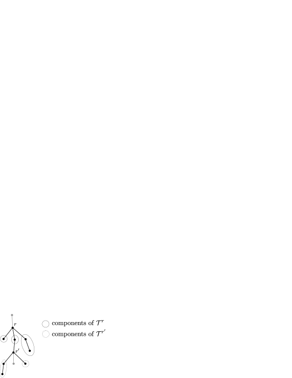
  Figure 8: The components $\mathcal{T}^{r}$ and $\mathcal{T}^{r^{\prime}}$. Vertices of $W_{X}$ are shown in gray.

  We embed the elements $t\in\mathcal{T}^{r^{\prime}}$ one after the other using Lemma 5.12. At each application of Lemma 5.12 we use $P=(X_{{\mathrm{L\ref{lemma_Embedding1}}}}\cap K\cap V^{\mathcal{Z}})\setminus\varphi(\mathcal{D}_{3})$, $P^{\prime}=P\cap\mathrm{N}(v)$, $Q=(Y_{{\mathrm{L\ref{lemma_Embedding1}}}}\cap K\cap V^{\mathcal{Z}})\setminus\varphi(\mathcal{D}_{3})$, and $Q^{\prime}=Q\cap\mathrm{N}(v)$. By (**), the vertex $v^{\prime}$ satisfies

  $$\deg(v^{\prime},(C\cap V^{\mathcal{Z}})\setminus\varphi(\mathcal{D}_{3})) \geq\frac{3\varepsilon s+\tau}{d-2\varepsilon}\;,\mbox{ and}$$

  $$\deg(v^{\prime},(D\cap V^{\mathcal{Z}})\setminus\mathcal{D}_{3})) \geq\frac{3\varepsilon s+\tau}{d-2\varepsilon}\;.$$

  By (A.12), we have that $\min\{|P^{\prime}|,|Q^{\prime}|\}\geq\frac{3\varepsilon s+\tau}{d-2\varepsilon}-\varepsilon s\geq\frac{\varepsilon s+\tau}{d-2\varepsilon s}$. We can thus use the “moreover” part of Lemma 5.12 to ensure that the root of $t$ (i.e. the unique vertex in $V(t)\cap\mathrm{N}_{F}(r^{\prime})$) is mapped to the set $P^{\prime}$.

  As we embedded $V(t_{i}^{j})\cap\mathrm{N}(W_{X})$ in $Z$ and the rest of $t_{i}^{j}$ in $(C\cup D)\cap V^{\mathcal{Z}}$, properties (I1), (I2), and (I3) trivially hold. As for (I4), we did not alter the set $\mathcal{Z}^{\prime}$ and the set $\varphi(\mathcal{D}_{3})$ may have only increased. Also observe that by (I3) we have that $|V(t_{i}^{j})\cap\mathrm{N}_{F}(W_{X})|\geq|\varphi(t_{i}^{j})\cap\bigcup\mathcal{Z}^{\prime}|$. Therefore, it is enough to show that if $\varphi$ was equable at the substep $j$, it is still equable at substep $j+1$ (i.e. after we embedded $t_{i}^{j}$). This was guaranteed by the choice of $X_{{\mathrm{L\ref{lemma_Embedding1}}}}$ and $Y_{{\mathrm{L\ref{lemma_Embedding1}}}}$, so that to minimise the difference between $|\varphi(\mathcal{D}_{3})\cap(C\cap V^{\mathcal{Z}})|$ and $|\varphi(\mathcal{D}_{3})\cap(D\cap V^{\mathcal{Z}})|$ together with the fact that $v(t_{i}^{j})\leq\tau$.

  Now consider the case when there is no cluster $Z\in\mathcal{Z}$ that satisfies (*) and (**). If $\varphi$ is equable and $\mathcal{Z}^{\prime}=\mathcal{Z}$ then we redefine $\mathcal{Z}^{\prime}$ to be the set of clusters in $\mathcal{Z}$ with respect to which the vertex $\varphi(x_{i})$ is typical and for which (*) holds. We want to check (I4) for this new set $\mathcal{Z}^{\prime}$.

  As $\varphi(x_{i})\in\tilde{X}$ by (I2), we have that $\varphi(x_{i})$ is typical to all but at most $\sqrt{\varepsilon}N$ clusters of $\mathcal{Z}$. Therefore,

  $$\mathrm{d\overline{eg}}_{\mathbf{H}}(X,\bigcup\mathcal{Z}^{\prime}) \geq\mathrm{d\overline{eg}}_{\mathbf{H}}(X,\bigcup\mathcal{Z})-\sqrt{\varepsilon}n-\left(|U_{i}^{j}\cap\bigcup(\mathcal{Z}\setminus\mathcal{Z}^{\prime})|+\frac{\xi n}{4}\right)$$

  $$\geq|V(\mathcal{D}_{3})\cap\mathrm{N}_{F}(W_{X})|-|U_{i}^{j}\cap\bigcup(\mathcal{Z}\setminus\mathcal{Z}^{\prime})|+\xi n-\sqrt{\varepsilon}n-\frac{\xi n}{4}$$

  $$\overset{\mbox{\tiny{{\bf(I3)}}}}{\geq}|(V(\mathcal{D}_{3})\cap\mathrm{N}_{F}(W_{X}))\setminus V_{i}^{j}|+|U_{i}^{j}\cap\bigcup\mathcal{Z}^{\prime}|+\frac{\xi n}{2}\;.$$

  By the definition of $\mathcal{Z}^{\prime}$, (**) does not hold for any cluster $Z\in\mathcal{Z}^{\prime}$. Then, as $\varphi$ is equable, we have

  $$\min \{\mathrm{d\overline{eg}}(Z,C\cap V^{\mathcal{Z}}),\mathrm{d\overline{eg}}(Z,D\cap V^{\mathcal{Z}})\}$$

  $$\leq\max\{|U_{i}^{j}\cap C\cap V^{\mathcal{Z}}|,|U_{i}^{j}\cap D\cap V^{\mathcal{Z}}|\}+\tau+\varepsilon s+\frac{3\varepsilon s+\tau}{d-2\varepsilon}$$

  $$\leq\min\{|U_{i}^{j}\cap C\cap V^{\mathcal{Z}}|,|U_{i}^{j}\cap D\cap V^{\mathcal{Z}}|\}+2\tau+\varepsilon s+\frac{3\varepsilon s+\tau}{d-2\varepsilon}$$

  $$\overset{\mbox{\tiny{{\bf(I3)}}}}{\leq}\min\{|\varphi(\mathcal{D}_{3})\cap C|,|\varphi(\mathcal{D}_{3})\cap D|\}+\frac{8\varepsilon s}{d}\;,$$

  showing that the newly created set $\mathcal{Z}^{\prime}$ satisfies (I4).

  So we may assume that the second condition of (I4) is satisfied. Let $Z\in\mathcal{Z}^{\prime}$ be a cluster as in Claim A.1.2 $(d)$ and map the root of $t_{i}^{j}$ to a vertex $v\in Z\cap\tilde{Z}$. Then pick an edge $CD\in M_{v}$ as in Claim A.1.3. Let $K\subseteq C\cup D$ be the set of vertices that are typical (where typicality refers to $C$ or $D$, respectively) w.r.t. $(Z\cap\tilde{Z})\setminus U_{i}^{j}$.

  Without loss of generality, assume that $|\mathrm{N}(v,K\cap D\cap V^{\mathcal{Z}}\setminus U_{i}^{j})|\leq|\mathrm{N}(v,K\cap C\cap V^{\mathcal{Z}}\setminus U_{i}^{j})|$. Let $X_{{\mathrm{L\ref{lemma_Embedding1}}}}=C$ and $Y_{{\mathrm{L\ref{lemma_Embedding1}}}}=D$. Consider the set $\mathcal{T}^{r}$ of components of $t_{i}^{j}-\mathrm{N}_{F}(W_{X})$ that are incident to $r$. We embed the elements $t\in\mathcal{T}^{r}$ one after the other using Lemma 5.12 with the following setting,

  $$P =(X_{{\mathrm{L\ref{lemma_Embedding1}}}}\cap K\cap V^{\mathcal{Z}})\setminus\varphi(\mathcal{D}_{3})\;, P^{\prime} =P\cap\mathrm{N}(v)\;,$$

  $$Q =(Y_{{\mathrm{L\ref{lemma_Embedding1}}}}\cap K\cap V^{\mathcal{Z}})\setminus\varphi(\mathcal{D}_{3})\;, Q^{\prime} =Q\cap\mathrm{N}(v)\;.$$

  By (A.8) we have $|(P^{\prime}\cup Q^{\prime})|\geq\frac{\xi s}{4}-2\varepsilon s$. As by assumption we have $|P^{\prime}|\geq|Q^{\prime}|$, we get $|P^{\prime}|\geq\frac{\xi s}{8}-\varepsilon s\geq\frac{\varepsilon s+\tau}{d-2\varepsilon}.$

  From (A.8) we derive

  $$|Q| \geq|\tilde{D}\cap V^{\mathcal{Z}}|-|(D\cap V^{\mathcal{Z}})\cap U_{i}^{j}|=|\tilde{D}\cap V^{\mathcal{Z}}|-|((C\cup D)\cap V^{\mathcal{Z}})\cap U_{i}^{j}|+|(C\cap V^{\mathcal{Z}})\cap U_{i}^{j}|$$

  $$\geq|\tilde{D}\cap V^{\mathcal{Z}}|-\left(\deg(v,(C\cup D)\cap V^{\mathcal{Z}})-2\tau-2\varepsilon s-\frac{\xi s}{2}\right)+|(C\cap V^{\mathcal{Z}})\cap U_{i}^{j}|$$

  $$=|\tilde{D}\cap V^{\mathcal{Z}}|-\max\left\{\deg(v,C\cap V^{\mathcal{Z}}),\deg(v,D\cap V^{\mathcal{Z}})\right\}+2\tau+2\varepsilon s+\frac{\xi s}{2}$$

  $$-\min\left\{\deg(v,C\cap V^{\mathcal{Z}}),\deg(v,D\cap V^{\mathcal{Z}})\right\}+\min\left\{|(C\cap V^{\mathcal{Z}})\cap U_{i}^{j}|,|(D\cap V^{\mathcal{Z}})\cap U_{i}^{j}|\right\}$$

  $$\geq 2\tau+\varepsilon s+\frac{\xi s}{2}-\left(\min\left\{\mathrm{d\overline{eg}}(Z,C\cap V^{\mathcal{Z}}),\mathrm{d\overline{eg}}(Z,D\cap V^{\mathcal{Z}})\right\}+\varepsilon s\right)$$

  $$+\min\left\{|(C\cap V^{\mathcal{Z}})\cap U_{i}^{j}|,|(D\cap V^{\mathcal{Z}})\cap U_{i}^{j}|\right\}$$

  $$\overset{\mbox{\tiny{{\bf(I4)}}}}{\geq}2\tau+\varepsilon s+\frac{\xi s}{2}-\varepsilon s\geq\frac{\varepsilon s+\tau}{d-2\varepsilon}\;.$$

  If $r$ is the only element in $V(t_{i}^{j})\cap\mathrm{N}_{F}(W_{X})$, then we are done with embedding $t_{i}^{j}$. Otherwise, let $r^{\prime}$ be the second vertex in $V(t_{i}^{j})\cap\mathrm{N}_{F}(W_{X})$. The predecessor of $r^{\prime}$ is mapped on a vertex $u\in K$ that is typical w.r.t. the set $(Z\cap\tilde{Z})\setminus U_{i}^{j}$ and hence satisfies (A.13). We can thus mapped the vertex $r^{\prime}$ to an unused vertex $v^{\prime}\in(Z\cap\tilde{Z})\cap\mathrm{N}(u)$ that is typical w.r.t. $C\cap V^{\mathcal{Z}}$ and typical w.r.t. $D\cap V^{\mathcal{Z}}$. Let $X_{{\mathrm{L\ref{lemma_Embedding1}}}}=C$ and $Y_{{\mathrm{L\ref{lemma_Embedding1}}}}=D$. Consider the set $\mathcal{T}^{r^{\prime}}$ of components of $t_{i}^{j}-\{r^{\prime}\}$ that are incident to $r^{\prime}$ and does not contain $r$. We embed the elements $t\in\mathcal{T}^{r^{\prime}}$ one after the other using Lemma 5.12 similarly as we did for the elements of $\mathcal{T}^{r}$. At each application of Lemma 5.12 we use $P=(X_{{\mathrm{L\ref{lemma_Embedding1}}}}\cap K\cap V^{\mathcal{Z}})\setminus\varphi(\mathcal{D}_{3})$, $P^{\prime}=P\cap\mathrm{N}(v^{\prime})$, $Q=(Y_{{\mathrm{L\ref{lemma_Embedding1}}}}\cap K\cap V^{\mathcal{Z}})\setminus\varphi(\mathcal{D}_{3})$, and $Q^{\prime}=Q\cap\mathrm{N}(v^{\prime})$.

  Observe that the embedding $\varphi$ satisfies (I1)–(I4).

∎

References

- [1] M. Ajtai, J. Komlós, and E. Szemerédi. On a conjecture of Loebl. In Graph theory, combinatorics, and algorithms, Vol. 1, 2 (Kalamazoo, MI, 1992), Wiley-Intersci. Publ., pages 1135–1146. Wiley, New York, 1995.
- [2] O. Barr and R. Johansson. Another Note on the Loebl–Komlós–Sós Conjecture. Research reports no. 22, (1997), Umeå University, Sweden.
- [3] C. Bazgan, H. Li, and M. Woźniak. On the Loebl-Komlós-Sós conjecture. J. Graph Theory, 34(4):269–276, 2000.
- [4] S. A. Burr. Generalized Ramsey theory for graphs—a survey. In Graphs and combinatorics (Proc. Capital Conf., George Washington Univ., Washington, D.C., 1973), pages 52–75. Lecture Notes in Mat., Vol. 406. Springer, Berlin, 1974.
- [5] O. Cooley. Proof of the Loebl-Komlós-Sós conjecture for large, dense graphs. Discrete Math., 309(21):6190–6228, 2009.
- [6] R. Diestel. Graph theory, volume 173 of Graduate Texts in Mathematics. Springer-Verlag, Berlin, third edition, 2005.
- [7] E. Dobson. Constructing trees in graphs whose complement has no . Combin. Probab. Comput., 11(4):343–347, 2002.
- [8] P. Erdős. Extremal problems in graph theory. In Theory of Graphs and its Applications (Proc. Sympos. Smolenice, 1963), pages 29–36. Publ. House Czechoslovak Acad. Sci., Prague, 1964.
- [9] P. Erdős, R. J. Faudree, C. C. Rousseau, and R. H. Schelp. Ramsey numbers for brooms. In Proceedings of the thirteenth Southeastern conference on combinatorics, graph theory and computing (Boca Raton, Fla., 1982), volume 35, pages 283–293, 1982.
- [10] P. Erdős, Z. Füredi, M. Loebl, and V. T. Sós. Discrepancy of trees. Studia Sci. Math. Hungar., 30(1-2):47–57, 1995.
- [11] J. W. Grossman, F. Harary, and M. Klawe. Generalized Ramsey theory for graphs. X. Double stars. Discrete Math., 28(3):247–254, 1979.
- [12] P. E. Haxell, T. Łuczak, and P. W. Tingley. Ramsey numbers for trees of small maximum degree. Combinatorica, 22(2):287–320, 2002. Special issue: Paul Erdős and his mathematics.
- [13] J. Hladký. Szemerédi Regularity Lemma and its applications in combinatorics. MSc. Thesis, Charles University, 2008, http://users.math.cas.cz/~hladky/papers.html.
- [14] J. Hladký, J. Komlós, D. Piguet, M. Simonovits, M. Stein, and E. Szemerédi. The approximate Loebl–Komlós–Sós Conjecture I: The sparse decomposition, 2014. arXiv:1408.3858.
- [15] J. Hladký, J. Komlós, D. Piguet, M. Simonovits, M. Stein, and E. Szemerédi. The approximate Loebl–Komlós–Sós Conjecture II: The rough structure of LKS graphs, 2014. arXiv:1408.3871.
- [16] J. Hladký, J. Komlós, D. Piguet, M. Simonovits, M. Stein, and E. Szemerédi. The approximate Loebl–Komlós–Sós Conjecture III: The finer structure of LKS graphs, 2014. arXiv:1408.3866.
- [17] J. Hladký, J. Komlós, D. Piguet, M. Simonovits, M. Stein, and E. Szemerédi. The approximate Loebl–Komlós–Sós Conjecture IV: Embedding techniques and the proof of the main result, 2014. arXiv:1408.3870.
- [18] J. Hladký, D. Piguet, M. Simonovits, M. Stein, and E. Szemerédi. The approximate Loebl–Komlós–Sós conjecture and embedding trees in sparse graphs. Electron. Res. Ann. Math. Sci., 22:1–11, 2015.
- [19] J. Komlós, A. Shokoufandeh, M. Simonovits, and E. Szemerédi. The regularity lemma and its applications in graph theory. In Theoretical aspects of computer science (Tehran, 2000), volume 2292 of Lecture Notes in Comput. Sci., pages 84–112. Springer, Berlin, 2002.
- [20] J. Komlós and M. Simonovits. Szemerédi’s regularity lemma and its applications in graph theory. In Combinatorics, Paul Erdős is eighty, Vol. 2 (Keszthely, 1993), volume 2 of Bolyai Soc. Math. Stud., pages 295–352. János Bolyai Math. Soc., Budapest, 1996.
- [21] D. Kühn and D. Osthus. Embedding large subgraphs into dense graphs. In Surveys in combinatorics 2009, volume 365 of London Math. Soc. Lecture Note Ser., pages 137–167. Cambridge Univ. Press, Cambridge, 2009.
- [22] D. Piguet and M. J. Stein. Loebl-Komlós-Sós conjecture for trees of diameter 5. Electron. J. Combin., 15(1):Research Paper 106, 11 pp. (electronic), 2008.
- [23] D. Piguet and M. J. Stein. An approximate version of the Loebl-Komlós-Sós conjecture. J. Combin. Theory Ser. B, 102(1):102–125, 2012.
- [24] M. Simonovits. A method for solving extremal problems in graph theory, stability problems. In Theory of Graphs (Proc. Colloq., Tihany, 1966), pages 279–319. Academic Press, New York, 1968.
- [25] S. N. Soffer. The Komlós-Sós conjecture for graphs of girth 7. Discrete Math., 214(1-3):279–283, 2000.
- [26] L. Sun. On the Loebl-Komlós-Sós conjecture. Australas. J. Combin., 37:271–275, 2007.
- [27] E. Szemerédi. Regular partitions of graphs. In Problèmes combinatoires et théorie des graphes (Colloq. Internat. CNRS, Univ. Orsay, Orsay, 1976), volume 260 of Colloq. Internat. CNRS, pages 399–401. CNRS, Paris, 1978.
- [28] Y. Zhao. Proof of the conjecture for large . Electron. J. Combin., 18(1):Paper 27, 61, 2011.