Leading Singularities of the Two-Loop Six-Particle MHV Amplitude

Abstract

We use the leading singularity technique to determine the planar six-particle two-loop MHV amplitude in ${\cal N}=4$ super Yang-Mills in terms of a simple basis of integrals. Our result for the parity even part of the amplitude agrees with the one recently presented in Bern:2008ap . The parity-odd part of the amplitude is a new result. The leading singularity technique reduces the determination of the amplitude to finding the solution to a system of linear equations. The system of equations is easily found by computing residues. We present the complete system of equations which determines the whole amplitude, and solve the two-by-two blocks analytically. Larger blocks are solved numerically in order to test the ABDK/BDS iterative structure.

I Introduction

Scattering amplitudes in massless gauge theories are remarkable objects with many properties hidden in the complexity of their Feynman diagram expansion. It has been known for decades that much information about an amplitude can be gleaned just from knowing the structure of its singularities (see SMatrix ). In Yang-Mills theories, extensive use of branch cut singularities was shown to tame much complexity in the computation of loop amplitudes via techniques that came to be known as the unitarity based method Bern:1994zx ; Bern:1994cg ; Bern:1995db ; Bern:1996je ; BDDKSelfDual ; Bern:1997sc ; Bern:2004cz .

One of the most surprising features of Yang-Mills theory and gravity is that their tree level amplitudes can be completely determined by exploiting only their behavior near a subset of their singularities BCFTree ; BCFW ; ArkaniHamed:2008yf . Another surprise, this time in ${\cal N}=4$ SYM, is that the problem of computing one-loop amplitudes can be reduced to that of computing tree amplitudes BCFLoop . The key to such striking simplification is that although the loop amplitude possesses poles and many branch cuts with a complicated structure of intersections, it is completely determined by the structure of the highest codimension singularities. These are known as the leading singularities SMatrix and are computed by cutting all propagators in the diagram.

Applying the same technique at higher loops was first attempted in Buchbinder:2005wp and refined in Bern:2007ct ; Cachazo:2008dx . In Buchbinder:2005wp and in Bern:2007ct both the leading singularity as well as subleading (i.e., lower codimension) singularities were used to constrain the form of higher loop amplitudes. In Cachazo:2008vp , the leading singularity was shown to be much more powerful than expected. It turns out that in massless theories, whenever all propagators are cut, one is actually studying many isolated singularities at the same time. The proposal of Cachazo:2008vp , building on observations made in Cachazo:2008dx , is to use each isolated singularity independently.

The new leading singularity technique outlined in Cachazo:2008vp has three notable features. Firstly, for any amplitude under consideration it builds a natural set of integrals, which we call the geometric integrals, that can be used to construct a basis. Secondly, the coefficients of the integrals can be determined by solving linear equations. Finally, these linear equations are easily obtained by computing residues using Cauchy’s theorem. The utility of this new technique was demonstrated in Cachazo:2008vp , where it was shown that it easily reproduces the result for the two-loop five-particle amplitude in ${\cal N}=4$ SYM previously computed in TwoLoopFiveB using the unitarity based method.

In this paper we apply the leading singularity technique to a much more challenging case, the planar two-loop six-particle MHV amplitude ${A}^{(2)}_{6,{\rm MHV}}$. The parity-even part of the normalized amplitude ${A}^{(2)}_{6,{\rm MHV}}/{A}^{\rm tree}_{6,{\rm MHV}}$ was computed recently in Bern:2008ap using the unitarity based method. This was already an impressive display of computational power. In the five particle case studied in TwoLoopFiveA ; TwoLoopFiveB the parity-odd part is noticeably of a higher degree of complexity than the parity-even part, and there is no reason to suspect that this would not be the case also for $n=6$. Here we find that the full coefficients (both the even and odd parts) emerge by solving the relatively simple linear equations presented explicitly below.

For six particles we find a new phenomenon which was not encountered in the $n=4,5$ cases studied in Cachazo:2008vp : while there are 177 geometric integrals, the equations only fix 159 linear combinations of their coefficients, leaving 18 linear combinations undetermined. The reason is that the set of geometric integrals is overcomplete, so we cannot have expected to find a unique solution. One can show that by using well-known techniques Melrose:1965kb ; vanNeerven:1983vr it is possible to build linear relations between seemingly independent integrals. In section IV we analyze the relevant reduction identities and identify 18 relations amongst the integrals in the geometric basis. Thus there is no ambiguity beyond that required by reduction identities, so we conclude that ${A}_{6,{\rm MHV}}^{(2)}$ is in fact completely determined by its leading singularities.

It is important to stress that the leading singularity method turns loop integrals into contour integrals which are finite in four dimensions and knows nothing about how one might choose to regulate the infrared divergences that typically appear when carrying out the loop integrals. In dimensional regularization, amplitudes occasionally contain additional terms in the integrand which vanish in $D=4$. These so-called “$\mu$-terms” (see for example Bern:2002tk for a thorough treatment) cannot be detected by the leading singularity in $D=4$.

One motivation for computing the MHV six-particle amplitude, beyond its serving as a testing ground for the leading singularity method, is to study the proposed iterative relation between MHV loop amplitudes known as the ABDK/BDS ansatz ABDK ; BDS . The ansatz has been shown to hold for four particles up to three loops ABDK ; BDS and for five particles up to two loops TwoLoopFiveA ; TwoLoopFiveB . However, it was shown to break down for the parity-even part of the two-loop six-particle MHV amplitude in Bern:2008ap . In this paper we find numerical evidence that the parity-odd part of the amplitude does satisfy the ABDK/BDS ansatz.

II Outline of the Calculation

The object of interest is the planar six-particle two-loop MHV amplitude in ${\cal N}=4$ super Yang-Mills. The goal is to find a compact expression for this amplitude as a linear combination of relatively simple integrals. The leading singularity method Cachazo:2008vp provides both a natural set of integrals to work with, as well as a system of linear equations which determine the coefficients of those integrals.

In this section we provide a detailed outline of the steps involved in setting up the calculation. The first three subsections are relevant to NMHV as well as MHV amplitudes, since the homogeneous part of the system of linear equations is helicity independent. In subsection II.D we compute the inhomogeneous terms for the MHV helicity configuration. The final linear equations which determine the coefficients of the MHV amplitude are presented explicitly in section III.

II.1 Review of the Leading Singularity Method

Suppose we are interested in calculating some $L$-loop scattering amplitude ${A}$. On the one hand, the amplitude may of course be represented as a sum over Feynman diagrams $F_{j}$,

$${A}(k)=\sum_{j}\int\prod_{a=1}^{L}d^{d}\ell_{a}\ F_{j}(k,\ell)\,,$$ (1)

where $k$ are external momenta and $\ell_{a}$ are the loop momenta. However it is frequently the case, especially in theories as rich as ${\cal N}=4$ SYM, that directly calculating the sum over Feynman diagrams would be impractical. Rather the calculation proceeds by expressing ${A}$ as a linear combination of relatively simple integrals in some appropriate basis $\{I_{i}\}$,

$${A}(k)=\sum_{i}c_{i}(k)\int\prod_{a=1}^{L}d^{d}\ell_{a}\ I_{i}(k,\ell)\,,$$ (2)

and then determining the coefficients $c_{i}$ by other means, such as the unitarity based method. If the set of integrals $\{I_{i}\}$ is overcomplete, then the coefficients $c_{i}(k)$ are not uniquely defined.

The basic idea underlying the leading singularity method is that the sum over Feynman diagrams in (1) possesses singularities which must be properly reproduced by any representation (2) of the amplitude in terms of simpler integrals. At the same time, any singularities in the set of integrals which are not present in the sum over Feynman diagrams must be spurious.

The most common kind of singularities in Feynman diagrams are poles, associated to collinear or multi-particle singularities, and branch cuts, associated to unitarity cuts. These branch cuts can themselves possess branch cuts leading to higher codimension singularities. The latter are computed by cutting propagators or equivalently Cachazo:2008dx by promoting the loop integral to be a contour integral. (The observation that the Lorentz invariant phase space integral of a null vector can be recast as a contour integral was first discussed in CSW .) The contour is chosen to reproduce the behavior of the delta-functions in the cut calculations. In general, this gives rise to contours which compute the residue on several isolated singularities at the same time.

For example, consider the one-loop massless scalar box. Replacing each propagator by a delta-function leads us to consider the integral

$$\int d^{4}\ell\,\delta(\ell^{2})\delta((\ell-k_{1})^{2})\delta((\ell-k_{1}-k_{2})^{2})\delta((\ell+k_{4})^{2})\,.$$ (3)

For generic external momenta $k_{i}$ these delta-functions localize the $\ell$ integral onto two discrete points in complex $\ell$-space ($\mathbb{C}^{4}$). With the leading singularity method we do not replace propagators by delta-functions, but rather we consider two separate $T^{4}$ contours in $\mathbb{C}^{4}$, each of which computes the residue of the integrand on only one of the two isolated singularities. Then by equating (1) and (2) and performing the integral

$$\sum_{i}c_{i}(k)\int_{\Gamma}d^{4}\ell\,I_{i}(k,\ell)=\int_{\Gamma}d^{4}\ell\,\sum_{j}F_{j}(k,\ell)$$ (4)

we obtain one linear equation on the coefficients $c_{i}$ for each contour $\Gamma$. At $L$ loops each contour is a $T^{4L}$ inside $\mathbb{C}^{4L}$. Since the number of isolated singularities in a generic $L$-loop diagram can be as high as $2^{L}$ (simple diagrams can have fewer isolated singularities), the leading singularity method gives rise to an exponentially large (in $L$) number of linear equations for the coefficients $c_{i}$. We note that the homogeneous part of these linear equations (the left-hand side of (4)) depends only on the set of integrals $\{I_{i}\}$ and the choice of contours, while the details of which particular helicity configuration is under consideration enters only into the inhomogeneous terms on the right-hand side.

II.2 Choosing Useful Contours

The formula (4) gives a linear equation on the coefficients $c_{i}$ for any contour $\Gamma$ in ${\mathbb{C}}^{4L}$. Of course if we choose some random contour $\Gamma$ then we will typically get the useless equation $0=0$. In order to get useful equations we should use $T^{4L}$ contours which calculate residues at the known singularities of the right-hand side. It is clear that in the sum over Feynman diagrams, singularities occur when internal propagators go on-shell.

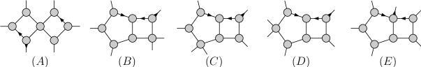
Figure 1: The five indepedent 8-propagator topologies. Each diagram represents a sum of those Feynman diagrams in which all of the 8 indicated propagators are present. In each diagram the external momenta are labeled clockwise beginning with $k_{1}$ at the position of the arrow. Also in each diagram $p$ is the loop momentum in the left loop and $q$ is the momentum in the right loop.

For six particles at two-loops there are two classes of useful $T^{8}$ contours. The most obvious $T^{8}$ contours are those which are chosen to calculate the residue at points in $\mathbb{C}^{8}$ where eight propagators go on-shell simultaneously. These contours are associated with the five different topologies shown in fig. 1. Actually each topology in fig. 1 is a diagrammatic shorthand for four distinct $T^{8}$ contours. For example, the singularities of Feynman diagrams with topology $(D)$ are situated at the locus

$$S_{(D)}=\{(p,q)\in\mathbb{C}^{4}\times\mathbb{C}^{4} : p^{2}=0,~{}(p+k_{6})^{2}=0,~{}(p+k_{456})^{2}=0,~{}(p-k_{12})^{2}=0,$$ (6)

$$q^{2}=0,~{}(q+k_{1})^{2}=0,~{}(q+k_{12})^{2}=0,~{}(p+q)^{2}=0\}\,.$$

For generic external momenta $k_{i}$ $S_{(D)}$ consists of four distinct points in $\mathbb{C}^{8}$ of the form $(p^{(i)},q^{(j)})$ for $i,j=1,2$. Correspondingly there are four different contours $\Gamma$ associated with topology $(D)$, one which computes the residue of the integrand at each of these four isolated singularities.

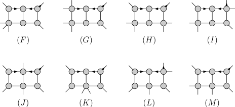
Figure 2: The eight independent 7-propagator topologies. See fig. 1 for details.

The less obvious $T^{8}$ contours are those in which only seven propagators are apparent but an eighth singularity appears due to a Jacobian. These contours are associated with the eight different topologies shown in fig. 2. For example, let us consider topology $(F)$. For fixed loop momentum $p$ the singularities in the $q$ integral occur at the locus

$$S_{(F)q}=\{q\in\mathbb{C}^{4}:q^{2}=0,~{}(q+k_{1})^{2}=0,~{}(q+k_{12})^{2}=0,~{}(q+p)^{2}=0\}\,,$$ (7)

which consists of two points $\{q^{(1)},q^{(2)}\}$ in $\mathbb{C}^{4}$. For each of these two singularities there is a contour $\Gamma_{q}$ such that integrating $q$ over $\Gamma_{q}$ computes the residue at that singularity. Integrating over either contour produces the same Jacobian factor

$$\int_{\Gamma_{q}}d^{4}q\ \frac{1}{q^{2}(q+k_{1})^{2}(q+k_{12})^{2}(q+p)^{2}}={1\over 2}{1\over(k_{1}+k_{2})^{2}(p-k_{1})^{2}}\,.$$ (8)

The new singularity $1/(p-k_{1})^{2}$ combines with the three remaining singularities manifest in topology $(F)$ so that the integral over $p$ can be localized by integrating over contours which compute the residue at the points

$$S_{(F)p}=\{p\in\mathbb{C}^{4}:p^{2}=0,~{}(p+k_{6})^{2}=0,~{}(p-k_{12})^{2}=0,~{}(p-k_{1})^{2}=0\}\,.$$ (9)

We proceed analagously for each of the eight topologies shown in fig. 2. In each case we first integrate the right-hand loop momentum $q$ and then use the additional singularity generated by the Jacobian to integrate the left-hand loop momentum $p$, thereby completely localizing the integral onto a set of discrete points.

For the MHV amplitude it turns out that the linear equations generated by the 13 types of contours described in figs. 1 and 2 are sufficient to uniquely determine all coefficients, although there certainly are additional contours that could be used to generate additional equations from (4). We have checked that a class of additional equations are indeed satisfied by the MHV coefficients, thus providing a strong consistency check on the coefficients obtained from solving the equations in section III.

II.3 The Geometric Integrals

Although equation (4) can be used to generate linear equations for coefficients in an arbitrary basis $\{I_{i}\}$, the leading singularity method suggests a natural set of integrals in which the left-hand side is easy to compute and the individual integrals have a geometric interpretation, in a sense we now explain.

Figure 3: The geometric integrals for the two-loop six-particle amplitude in ${\cal N}=4$ SYM. In each diagram the external momenta are labeled clockwise beginning with $k_{1}$ at the position of the arrow and the number in parentheses denotes the number of independent permutations of the diagrams. As discussed in section IV, this is an overcomplete set: the 177 integrals here obey 18 linear relations.

The procedure to determine the natural set of integrals in which to represent an amplitude starts by realizing that in ${\cal N}=4$ SYM tadpoles, bubbles, and triangles are unneccesary (see Bern:2006ew for a thorough discussion). This means that we have to start by considering all topologies of sums over Feynman diagram with no triangles or bubbles. At one-loop, only sums of Feynman diagrams with the topology of a box are needed. For six particles at two-loops, we find five topologies with eight propagators, shown in fig. 1, and eight topologies with seven propagators, shown in fig. 2.

After each topology is identified, a first approximation for reproducing all of the leading singularities is to use just the scalar integrals with all of the appropriate topologies. In general, it turns out that such integrals are not enough to reproduce the singularities of Feynman diagrams. This will manifest itself in the failure of the linear equations (4) to have any solutions, indicating that the set of integrals must be enlarged.

The next step is to introduce scalar integrals with additional propagators. At one-loop this step gives rise to pentagons in addition to boxes, which turns out to be sufficient for any $n$. At two loops we add the scalar pentagon-pentagon integrals shown in fig. 3. At this stage some of the equations are solved (i.e. some of the leading singularities are correctly reproduced), while others are not.

It is then necessary to supplement additional integrals which must have non-zero residue on the missing singularities and zero residue on the ones which already work, in order to avoid spoiling them. The way to ensure that one has zero residue on a given pole is to include a zero in the numerator of the integrand which cancels the corresponding pole. In this form integrals with scalar numerators appear. Note that only numerators which cancel poles appear naturally.

The process of expanding the set of integrals by including additional numerator factors ends when one is able to solve all of the equations (4). We call the integrals that are naturally constructed in this manner geometric integrals. The set of geometric integrals might be overcomplete if the equations do not determine a unique solution. For the six-particle MHV amplitude at two loops this process leads to the 177 geometric integrals shown in fig. 3. For NMHV amplitudes it is possible that additional integrals, such as a pentagon-boxes with two numerators, might be required.

II.4 The Inhomogeneous Terms for the MHV Amplitude

As mentioned above, it is obvious from (4) that the homogeneous part of the system of linear equations is helicity independent, so the above discussion of the contours and geometric integrals applies to both the MHV and NMHV configurations. The inhomogeneous part on the right-hand side of (4) is easily obtained for any contour $\Gamma$ by computing the product of tree amplitudes sitting at the ‘blobs’ in the corresponding topology in fig. 1 or fig. 2. This product is evaluated at the value $(p^{(i)},q^{(j)})$ of the loop momenta where the contour $\Gamma$ localizes the integral.

For MHV configurations there is an enormous simplification since it turns out that this product of tree amplitudes always comes out to be $0$ or $1$ times the corresponding tree-level amplitude, as can easily be shown by using the technique introduced in Cachazo:2008dx where sums over the full ${\cal N}=4$ supermultiplet in the internal lines, which complicate the computation Buchbinder:2005wp ; Bern:2007ct , are automatically done by using simple identities.

For the contours associated with the 13 topologies shown in figs. 1 and 2 we find that the right-hand side of (4) for an MHV configuration are

$$(A): \qquad\delta_{\langle p,1\rangle}\delta_{\langle q,4\rangle}A^{\rm tree}_{6,{\rm MHV}}\,,$$ (10)

$$(B): \qquad\delta_{\langle p,6\rangle}\delta_{\langle q,1\rangle}A^{\rm tree}_{6,{\rm MHV}}\,,$$ (11)

$$(C): \qquad 0\,,$$ (12)

$$(D): \qquad\delta_{\langle p,6\rangle}A^{\rm tree}_{6,{\rm MHV}}\,,$$ (13)

$$(E): \qquad\delta_{\langle p,6\rangle}\delta_{\langle q,2\rangle}A^{\rm tree}_{6,{\rm MHV}}\,,$$ (14)

$$(F): \qquad\delta_{\langle p,6\rangle}A^{\rm tree}_{6,{\rm MHV}}\,,$$ (15)

$$(G): \qquad 0\,,$$ (16)

$$(H): \qquad 0\,,$$ (17)

$$(I): \qquad\delta_{\langle p,6\rangle}\delta_{\langle p,q\rangle}A^{\rm tree}_{6,{\rm MHV}}\,,$$ (18)

$$(J): \qquad 0\,,$$ (19)

$$(K): \qquad\delta_{[p,6]}\delta_{[q,1]}A^{\rm tree}_{6,{\rm MHV}}\,,$$ (20)

$$(L): \qquad 0\,,$$ (21)

$$(M): \qquad 0\,.$$ (22)

The Kronecker deltas such as $\delta_{\langle p,1\rangle}$ for topology $(A)$ arise because, in that example, the solution for $p$ is either of the form $\lambda_{p}\propto\lambda_{1}$ or $\widetilde{\lambda}_{p}\propto\widetilde{\lambda}_{1}$, and the product of tree amplitudes vanishes on latter solution.

III The MHV Equations and Their Solutions

We now assemble all of the ingredients prepared in section II for the MHV amplitude. By evaluating (4) on all of the contours associated with the topologies shown in figs. 1 and 2 (together with all of their cyclic and mirror-image permutations), and using (10) on the right-hand side, we find a system of 396 linear equations for the 177 coefficients of the geometric integrals in fig. 3.

Generically, 396 linear equations in 177 variables have no solution, but in this case we find that the equations are in fact underdetermined: they only fix 159 linear combinations of the 177 coefficients, leaving 18 free parameters. In other words, we find that there are 18 linear combinations of the geometric integrals in fig. 3 which have vanishing leading singularity on all of the contours described by figs. 1 and 2. One logically possible conclusion from such a result might have been that the leading singularity method is not enough to uniquely determine the two-loop six-particle MHV amplitude, which would have been disappointing.

Fortunately, as mentioned in the introduction, it turns out that integral reduction identities imply that the set of geometric integrals is overcomplete. In other words, there are linear combinations of the 177 geometric integrals which not only have vanishing leading singularity but actually vanish identically. In section IV we analyze these reduction identities and show that there are 18 linear combinations of the geometric integrals which vanish, precisely accounting for the abovementioned ambiguity in solving the leading singularity equations. The conclusion is therefore that the two-loop six-particle MHV amplitude is in fact uniquely determined by knowledge of its leading singularities.

III.1 Presentation of the Equations

In order to demonstrate that the leading singularity method is not just black magic, we present here explicit expressions for the equations which determine all coefficients $A^{(2)}_{6,{\rm MHV}}$, including both the parity-even and odd terms. As just discussed, 18 coefficients out of 177 are actually redundant. In order to somewhat simplify the presentation of the equations we will choose a convenient ‘gauge’ which uniquely fixes all of the ambiguity. This amounts to choosing a basis of geometric integrals.

Several such choices are possible; the choice we make here is to spend the 18 gauge parameters by setting to zero the 6 coefficients $c_{12}$ and the 12 coefficients $c_{24}$. Once this is done all remaining coefficients are uniquely determined. A nice advantage of this choice is that several other coefficients turn out to also vanish identically: the 12 coefficients $c_{22}$, the 12 coefficients $c_{18}$, the 6 coefficients $c_{16}$ and the 3 coefficients $c_{23}$ are all zero.

Ultimately then there are only 126 nonzero coefficients, associated with just 15 out of the 21 integrals shown in fig. 3. We label the $j$-th permutation of coefficient $c_{i}$ as $c_{i}^{(j)}$. Permutation $j$ maps the labeling $(1,2,3,4,5,6)$ of the external momenta to:

$$1:(1,2,3,4,5,6)\,,\quad~{}2:(2,3,4,5,6,1)\,,\quad~{}3:(3,4,5,6,1,2)\,,\quad~{}~{}4:(4,5,6,1,2,3)\,,$$

$$5:(5,6,1,2,3,4)\,,\quad~{}6:(6,1,2,3,4,5)\,,\quad~{}7:(6,5,4,3,2,1)\,,\quad~{}~{}8:(5,4,3,2,1,6)\,,$$

$$9:(4,3,2,1,6,5)\,,\quad 10:(3,2,1,6,5,4)\,,\quad 11:(2,1,6,5,4,3)\,,\quad 12:(1,6,5,4,3,2)\,.\quad$$ (23)

Since all of the coefficients for the MHV amplitude are proportional to the tree amplitude, we can go ahead and divide the right-hand side of all equations by $A^{\rm tree}_{6,{\rm MHV}}$. Equivalently we can say that solving the equations below yields the integral coefficients for the normalized amplitude $A^{(2)}_{6,{\rm MHV}}/A^{\rm tree}_{6,{\rm MHV}}$. A final comment is that we move all of the Jacobian factors (see for example eq. (8)) to the right-hand side of the equations.

Finally we are ready to present the equations obtained by considering the contours associated with the topologies in figs. 1 and 2. In each equation $p$ and $q$ are understood to be evaluated at the locations $(p^{(i)},q^{(j)})$ of all the leading singularities.

Topology A:

$$c_{1}^{(2)}+\frac{(p-k_{234})^{2}(q-k_{34})^{2}c_{13}^{(2)}+(p+k_{61})^{2}(q-k_{234})^{2}c_{13}^{(5)}}{(p+q-k_{234})^{2}}=4s_{12}s_{23}s_{45}s_{56}\delta_{\langle p,1\rangle}\delta_{\langle q,4\rangle}$$ (24)

Topology D:

$$c_{19}^{(2)}+(p-k_{1})^{2}c_{8}^{(6)}=4s_{12}(p-k_{1})^{2}(s_{123}s_{345}-s_{12}s_{45})\delta_{\langle p,6\rangle}$$ (25)

Topology E:

$$c_{21}^{(3)}+(p-k_{12})^{2}c_{10}^{(3)}+\frac{(p-k_{12})^{2}(q+k_{234})^{2}c_{13}^{(2)}+(p-k_{1})^{2}(q-k_{61})^{2}c_{13}^{(5)}}{(q-k_{1})^{2}}$$ (26)

$$\qquad\qquad=4s_{23}s_{45}s_{56}(p-k_{12})^{2}\delta_{\langle p,6\rangle}\delta_{\langle q,2\rangle}$$ (27)

Topology F:

$$c_{2}^{(6)}+\frac{c_{19}^{(2)}}{(p+k_{456})^{2}}=4s_{12}^{2}s_{61}\delta_{\langle p,6\rangle}$$ (28)

Topology H:

$$c_{4}^{(6)}+\frac{(p-k_{12})^{2}(q-k_{56})^{2}c_{13}^{(2)}+(p-k_{1})^{2}(q-k_{6})^{2}c_{13}^{(5)}}{(p+k_{56})^{2}(q+k_{12})^{2}}$$ (29)

$$+\frac{c_{20}^{(6)}+(q-k_{6})^{2}c_{9}^{(6)}}{(q+k_{12})^{2}}+\frac{c_{20}^{(12)}+(p-k_{1})^{2}c_{9}^{(12)}}{(p+k_{56})^{2}}=0$$ (30)

Topology I:

$$c_{3}^{(6)}+\frac{(p-k_{12})^{2}(q-k_{56})^{2}c_{13}^{(2)}+(p-k_{1})^{2}(q-k_{6})^{2}c_{13}^{(5)}}{(p+k_{56})^{2}(q+k_{1})^{2}}$$ (31)

$$+\frac{c_{20}^{(6)}+(q-k_{6})^{2}c_{9}^{(6)}}{(q+k_{1})^{2}}+\frac{c_{20}^{(3)}+(p-k_{12})^{2}c_{9}^{(3)}}{(p+k_{56})^{2}}=4s_{123}(s_{123}s_{345}-s_{12}s_{45})\delta_{\langle p,6\rangle}\delta_{\langle p,q\rangle}$$ (32)

Topology J:

$$c_{7}^{(5)}+\frac{c_{21}^{(12)}+(p-k_{61})^{2}c_{10}^{(12)}}{(p-k_{6})^{2}}+\frac{c_{21}^{(5)}+(q-k_{56})^{2}c_{10}^{(5)}}{(q-k_{6})^{2}}$$ (33)

$$+\frac{(p+k_{345})^{2}(q-k_{56})^{2}c_{13}^{(2)}+(p-k_{61})^{2}(q-k_{6})^{2}c_{13}^{(5)}}{(p-k_{6})^{2}(q+k_{123})^{2}}$$ (34)

$$+\frac{c_{21}^{(2)}+(p-k_{61})^{2}c_{10}^{(2)}}{(p+k_{345})^{2}}+\frac{c_{21}^{(9)}+(q-k_{56})^{2}c_{10}^{(9)}}{(q+k_{123})^{2}}$$ (35)

$$+\frac{(p-k_{61})^{2}(q-k_{456})^{2}c_{13}^{(1)}+(p-k_{6})^{2}(q-k_{56})^{2}c_{13}^{(4)}}{(p+k_{345})^{2}(q-k_{6})^{2}}=0$$ (36)

Topology K:

$$c_{17}^{(6)}+\frac{+(p-k_{12})^{2}(q-k_{56})^{2}c_{13}^{(2)}+(p-k_{1})^{2}(q-k_{6})^{2}c_{13}^{(5)}}{(p+k_{456})^{2}(q+k_{123})^{2}}$$ (37)

$$+\frac{c_{21}^{(6)}+(q-k_{6})^{2}c_{10}^{(6)}}{(q+k_{123})^{2}}+\frac{c_{21}^{(12)}+(p-k_{1})^{2}c_{10}^{(12)}}{(p+k_{456})^{2}}=4s_{12}s_{56}(q-k_{6})^{2}\delta_{\langle p,q\rangle}$$ (38)

Topology L:

$$c_{5}^{(3)}+\frac{(p-k_{12})^{2}(q-k_{56})^{2}c_{13}^{(2)}+(p-k_{1})^{2}(q-k_{6})^{2}c_{13}^{(5)}}{(p+k_{456})^{2}(q+k_{1})^{2}}$$ (39)

$$+\frac{c_{21}^{(6)}+(q-k_{6})^{2}c_{10}^{(6)}}{(q+k_{1})^{2}}+\frac{c_{20}^{(3)}+(p-k_{12})^{2}c_{9}^{(3)}}{(p+k_{456})^{2}}=0$$ (40)

Topology M:

$$c_{6}^{(6)}+\frac{(p-k_{12})^{2}(q-k_{56})^{2}c_{13}^{(2)}+(p-k_{1})^{2}(q-k_{6})^{2}c_{13}^{(5)}}{(p+k_{56})^{2}(q+k_{123})^{2}}$$ (41)

$$+\frac{c_{21}^{(12)}+(p-k_{1})^{2}c_{10}^{(12)}}{(p+k_{56})^{2}}+\frac{c_{20}^{(6)}+(q-k_{6})^{2}c_{9}^{(6)}}{(q+k_{123})^{2}}+\frac{c_{19}^{(2)}+(p-k_{1})^{2}c_{8}^{(2)}}{(p-k_{12})^{2}}=0$$ (42)

The equations for topologies $(B)$, $(C)$ and $(G)$ turn out to be redundant for the MHV amplitude with the choice of basis described above.

III.2 Analytic Results for a $2\times 2$ Block

The structure of the equations is sufficiently complicated that it is not clear whether it is possible to find useful analytic solutions, so in practice we resort to solving them numerically. However the equations from topologies ${(D)}$ and ${(F)}$ are exceptionally simple and only involve the coefficients $c_{2}$, $c_{8}$ and $c_{19}$, so they can easily be solved analytically as we now demonstrate.

III.2.1 Topology $(F)$

The four contour integrals for topology $(F)$ localize the integral at the four points $(p^{(i)},q^{(j)})_{i,j=1,2}$ given by

$$q^{(1)}=\left(-\lambda_{1}+\frac{\langle 1,6\rangle}{\langle 2,6\rangle}\lambda_{2}\right)\widetilde{\lambda}_{1}\,, \qquad p^{(1)}=\frac{\langle 2,1\rangle}{\langle 2,6\rangle}\lambda_{6}\widetilde{\lambda}_{1}\,$$ (43)

$$q^{(2)}=\lambda_{1}\left(-\widetilde{\lambda}_{1}+\frac{[1,6]}{[2,6]}\widetilde{\lambda}_{2}\right)\,, \qquad p^{(2)}=\frac{[2,1]}{[2,6]}\lambda_{1}\tilde{\lambda}_{6}\,.$$ (44)

Equation (28) is then

$$c_{2}^{(6)}+\frac{c_{19}^{(2)}}{(p^{(1)}+k_{456})^{2}}=4s_{12}^{2}s_{61}\,,\qquad c_{2}^{(6)}+\frac{c_{19}^{(2)}}{(p^{(2)}+k_{456})^{2}}=0\,.$$ (45)

Note that even though there are four different contours we only obtain two independent equations since (28) is independent of $q$. This is a generic feature whenever a contour is such that it chops off a massless box Cachazo:2008vp .

Solving (45) yields the coefficients

$$c_{2}^{(6)}={4s_{12}^{2}s_{61}\over 1-a},\qquad c_{19}^{(2)}={4s_{12}^{2}s_{61}\over 1-a}(p^{(1)}+k_{456})^{2}\,$$ (46)

where

$$a=\frac{(p^{(1)}+k_{456})^{2}}{(p^{(2)}+k_{456})^{2}}\,.$$ (47)

It is frequently useful to separate coefficients into their parity-even and parity-odd parts. Since parity exchanges $\langle i,j\rangle\leftrightarrow[i,j]$, it evidently takes $a\to 1/a$. If we denote the parity conjugate of a coefficient $c$ by $\bar{c}$ then we see that the even and odd parts of $c_{2}^{(6)}$ and $c_{19}^{(2)}$ are simply

$${1\over 2}(c_{2}^{(6)}+\bar{c}_{2}^{(6)})=2s_{16}s_{12}^{2}\,, \qquad{1\over 2}(c_{2}^{(6)}-\bar{c}_{2}^{(6)})=2s_{16}s_{12}^{2}\left(\frac{1+a}{1-a}\right)\,,$$ (48)

$${1\over 2}(c_{19}^{(2)}+\bar{c}_{19}^{(2)})=0\,, \qquad{1\over 2}(c_{19}^{(2)}-\bar{c}_{19}^{(2)})=4s_{12}^{2}s_{61}\frac{(p^{(1)}+k_{456})^{2}}{1-a}\,.$$ (49)

The parity-even parts of these coefficients agree precisely with those obtained in Bern:2008ap via the unitarity based method. Here we see that these coefficients can be obtained simply by solving two equations in two variables, and moreover the parity-odd parts automatically come along for free.

III.2.2 Topology ${(D)}$

For topology $(D)$ the contour integrals localize the integral at the points

$$p^{(1)}=(\alpha\lambda_{6}+\beta\lambda_{3})\widetilde{\lambda}_{6}\, \qquad q^{(1)}=\frac{[1,2]}{[2,6]}\lambda_{1}\widetilde{\lambda}_{6}\,,$$ (50)

$$p^{(2)}=\lambda_{6}({\alpha}\widetilde{\lambda}_{6}+\gamma\widetilde{\lambda}_{3})\, \qquad q^{(2)}=\frac{\langle 1,2\rangle}{\langle 2,6\rangle}\lambda_{6}\widetilde{\lambda}_{1}\,,$$ (51)

where

$$\alpha=\frac{s_{13}+s_{23}}{s_{36}},\quad\beta=\frac{-s_{12}+\alpha(s_{12}+s_{26})}{\langle 3|1+2|6]},\quad\gamma=\frac{-s_{12}+\alpha(s_{12}+s_{26})}{[3|1+2|6\rangle}\,.$$ (52)

Equation (25) then gives

$$c_{19}^{(2)}+\frac{c_{8}^{(6)}}{(p^{(1)}-k_{1})^{2}}=4s_{12}(s_{345}s_{456}-s_{12}s_{45})\,\qquad c_{19}^{(2)}+\frac{c_{8}^{(6)}}{(p^{(2)}-k_{1})^{2}}=0\,.$$ (53)

We can eliminate $c_{19}^{(2)}$ to solve for $c_{8}^{(6)}$, finding

$${1\over 2}(c_{8}^{(6)}+\bar{c}_{8}^{(6)}) = 2s_{12}(s_{123}s_{345}-s_{12}s_{45})\,$$ (54)

$${1\over 2}(c_{8}^{(6)}-\bar{c}_{8}^{(6)}) = 2s_{12}(s_{123}s_{345}-s_{12}s_{45})\left(\frac{c+1}{c-1}\right)\,,$$ (55)

where

$$c=\frac{(p^{(1)}-k_{1})^{2}}{(p^{(2)}-k_{1})^{2}}\,.$$ (56)

Again the even part of $c_{8}$ agrees precisely with the unitary based calculation of Bern:2008ap . Of course the equation (53) provides a consistency condition on the coefficient $c_{19}^{(2)}$ that we already obtained in (46).

III.3 The Parity-Even Part

In the previous subsection we solved for the coefficients $c_{2}$, $c_{8}$ and $c_{19}$ analytically and demonstrated that their parity-even parts agree with the results of Bern:2008ap . In order to check the validity of the leading singularity method it is important for us to compare the parity-even parts of all remaining coefficients as well. The first obstacle is the fact that Bern:2008ap used a basis containing the integral shown in fig. 4. According to our criteria we do not consider this a geometric integral since the propagator does not serve to cancel any pole. (The motivation for using $I_{11}$ in Bern:2008ap was that the integral is manifestly dual conformally invariant Drummond:2006rz ; DrummondVanishing .)

We show in the next section that reduction identities can be used to express $I_{11}$ as a linear combination of geometric integrals, so secretly fig. 3 already contains $I_{11}$. However in order to facilicate comparison of our results with those of Bern:2008ap it is convenient to explicitly add $I_{11}$ to the set of integrals. Then we have a set of $177+12=189$ integrals which is overcomplete by $18+12=30$ elements. Encouragingly, we find that it is possible to find a solution of the equations in which the non-dual conformally invariant integrals $I_{19}$–$I_{24}$ all have coefficients whose parity-even part vanishes. This is a necessary condition for agreement with Bern:2008ap since the parity-even part of the amplitude was expressed there in terms of dual conformally invariant integrals. Moreover we find that after choosing this ‘gauge’ there is no further ambiguity in the basis; the linear equations furnish a unique solution.

Figure 4: An extra 12 integrals we add to the set of geometric integrals in order to facilitate comparison with Bern:2008ap . These integrals are dual conformally invariant but not geometric. Nevertheless they can be expressed as linear combinations of the geometric integrals in fig. 3 using first class identities (see section IV).

As indicated above, the equations are sufficiently complicated that we found it necessary to solve them numerically. Let us note however that by ‘numerically’ we always mean that we choose all of the spinors $\lambda_{i},\widetilde{\lambda}_{i}$ to be random rational numbers (subject to momentum conservation, of course). Then the coefficients obtained by solving the equations always come out to be rational numbers, so they can be compared to the results of Bern:2008ap with absolute precision. By repeated successful comparison for many different random values of the spinors, we are able to report complete agreement with the parity-even parts of the coefficients obtained from the leading singularity method with those obtained in Bern:2008ap , recorded here in the $(1)$ permutation:

$$c_{1} = s_{61}s_{34}s_{123}s_{345}+s_{12}s_{45}s_{234}s_{345}+s_{345}^{2}(s_{23}s_{56}-s_{123}s_{234})\,,$$ (57)

$$c_{2} = 2s_{12}s_{23}^{2}\,,$$ (58)

$$c_{3} = s_{234}(s_{123}s_{234}-s_{23}s_{56})\,,$$ (59)

$$c_{4} = s_{12}s_{234}^{2}\,,$$ (60)

$$c_{5} = s_{34}(s_{123}s_{234}-2s_{23}s_{56})\,,$$ (61)

$$c_{6} = -s_{12}s_{23}s_{234}\,,$$ (62)

$$c_{7} = 2s_{123}s_{234}s_{345}-4s_{61}s_{34}s_{123}-s_{12}s_{45}s_{234}-s_{23}s_{56}s_{345}\,,$$ (63)

$$c_{8} = 2s_{61}(s_{234}s_{345}-s_{61}s_{34})\,,$$ (64)

$$c_{9} = s_{23}s_{34}s_{234}\,,$$ (65)

$$c_{10} = s_{23}(2s_{61}s_{34}-s_{234}s_{345})\,,$$ (66)

$$c_{11} = s_{12}s_{23}s_{234}\,,$$ (67)

$$c_{12} = s_{345}(s_{234}s_{345}-s_{61}s_{34})\,,$$ (68)

$$c_{13} = -s_{345}^{2}s_{56}\,.$$ (69)

However, as mentioned in the introduction we note that the leading singularity method is completely blind to the integrals $I_{14}$ and $I_{15}$ in Bern:2008ap since they have integrands that vanish in $D=4$.

IV Reductions

IV.1 Methods of Reduction

Repeatedly throughout the paper we have mentioned and used the new feature that happens for six or more particles; loop integrals often satisfy linear relations which can be used to write one in terms of others (see for example vanNeerven:1983vr , as well as Bern:1993kr for dimensionally regulated versions). Interestingly, there are relations even among what we call geometric integrals. Also important for us will be relations among integrals that appear in the manifestly dual conformal invariant expression of Bern:2008ap and our geometric integrals.

In this section we discuss in detail how these relations arise since it is a crucial step in completing the proof that the leading singularity method does determine the amplitude uniquely. Recall that out of the $177$ coefficients the leading singularity fixes $159$ thus leaving $18$ free parameters. We will now account for these as a consequence of relations or what we call reduction identities. In other words, the set of geometric integrals which naturally appears in the process of matching leading singularities is overcomplete.

We distinguish between two different kind of identities; the ones that are valid on any contour of integration and the ones that are valid only on $T^{8}$ contours where loop momenta can be taken to be in four-dimensions. We call these first and second class identities, respectively.

IV.1.1 First Class

Identities of the first class are those which are valid on any contour of integration, in particular, on the real contours where integrals must be regulated, e.g. using dimensional regularization.

First consider for example the pentagon-box integral

with numerator factor $(p-k_{1})^{2}$, which is a permutation of the one shown in fig. 4. Clearly, this integral is not geometric since the numerator is not a zero which cancels a pole of the integral. However, this integral is dual conformal invariant and it appears in the representation of the even part of the amplitude obtained in Bern:2008ap . The goal is to write this integral as a linear combination of the geometric integrals in fig. 3.

Let us write the numerator as $p^{2}-2k_{1}\cdot p$. The first term cancels a propagator and gives rise to a double-box integral of type $I_{17}$ in fig. 3. The second term can be decomposed by using that external momenta are kept in four dimensions. This means that only the four-dimensional component, $p_{[4]}$, of $p$ contributes, i.e. $k_{1}\cdot p=k_{1}\cdot p_{[4]}$. Given any four dimensional vector, one can write it as a linear combination of four axial vectors

$$\vartheta_{i}^{\mu}=\epsilon^{\mu\nu\rho\sigma}\ell^{i+1}_{\nu}\ell^{i+2}_{\rho}\ell^{i+3}_{\sigma}$$ (70)

where $\ell^{i}$, with $i=1,\ldots,4$, form a basis of four-vectors. In the case of interest, we choose to write $p_{[4]}$ as

$$p_{[4]}^{\mu}=\frac{1}{\epsilon^{\mu\nu\rho\sigma}\ell_{\mu}^{1}\ell^{2}_{\nu}\ell^{3}_{\rho}\ell^{4}_{\sigma}}\sum_{i=1}^{4}(p_{[4]}\cdot\ell_{i})\vartheta_{i}^{\mu}$$ (71)

with the choice

$$\ell_{1}=k_{6}\,,\quad\ell_{2}=k_{5}+k_{6}\,,\quad\ell_{3}=k_{4}+k_{5}+k_{6}\,,\quad\ell_{4}=-k_{1}-k_{2}\,.$$ (72)

This a standard construction in the scattering amplitude literature vanNeerven:1983vr ; Bern:1993kr .

Since all of the $\ell_{i}$ are written in terms of external particle momenta, they are completely four-dimensional so we are free to replace $p_{[4]}$ by $p$ in the coefficients $(p_{[4]}\cdot\ell_{i})$. Writing each coefficient as $2p\cdot\ell_{i}=(p+\ell_{i})^{2}-p^{2}-\ell_{i}^{2}$, one finds that the term $k_{1}\cdot p$ in the original integral can be decomposed in terms of numerators which give rise to geometric integrals. Perhaps the only term which might require some explanation is the one corresponding to $\ell_{4}=-k_{1}-k_{2}$ since it is one which does not cancel a propagator. In this case the factor $(p-k_{1}-k_{2})^{2}$ becomes a numerator which is easily seen to be a zero that cancels a pole which removes a leading singularity and hence gives rise to a geometric integral.

From this example it is clear what the necessary conditions are for the existence of first class relations among integrals. The first condition is that there be at least four propagators (including $1/p^{2}$) involving the same loop variable and only external momenta. If the number of such propagators is exactly four then there must be at least two different ways of putting a numerator which only involves the loop variable of interest and external momenta. This was the case considered above. If the number of propagators is at least five, then a relation can be obtained if at least one numerator is available. If the number of propagators is six or more, then no numerators are needed.

In our case, with six external particles, the maximum number of propagators in a single loop which only depend on a single loop variable and external momenta is five. This diagram is a hexagon-box. In fact, it is easy to show that a hexagon-box with a numerator can be reduced. We leave this as an exercise for the reader since such an integral did not have to be included in the original set of geometric integrals, at least in the MHV case.

Using identities of the first class we will be able to show that all six $I_{12}$ integrals can be written in terms of $I_{13}$ integrals plus other geometric integrals. This shows $6$ of the $18$ relations we have to account for. Also using first class relations we will show that $6$ of the $12$ $I_{24}$ integrals can be written in terms of the remaining six and other geometric integrals. Summarizing, after using all first class identities we end up with $6$ relations left to explain. These turn out to be second class identities.

IV.1.2 Second Class

The identities discussed above are valid in any contour because the loop momentum is always contracted with external momenta and hence it can be treated effectively as four dimensional. We now turn to identities which only hold on the $T^{8}$ contours where the loop momentum integrals can be taken completely in four dimensions. These identities will not hold in dimensional regularization. In fact, their failure to hold exactly is precisely proportional to integrals with numerators made out of the $-2\epsilon$-dimensional component of the loop momenta. We obtain identities by reducing integrals of this type to find linear combinations of other integrals which must sum to zero for four dimensional loop momenta.

Consider first an integral with numerator, $p_{[-2\epsilon]}\cdot q_{[-2\epsilon]}=p\cdot q-p_{[4]}\cdot q_{[4]}$. The first term can be written as $2p\cdot q=(p+q)^{2}-p^{2}-q^{2}$. In order to treat the second term one has to find a convenient basis to expand $p_{[4]}$ and one for $q_{[4]}$. The relevant diagram must have at least four propagators that only depend on $p$ and at least four that only depend on $q$ and external momenta. With six external particles there is only one possible diagram (up to relabeling). This is the double pentagon integral

Let us choose to write $p_{[4]}^{\mu}$ using the reference vectors

$$\ell_{1}=k_{6}\,,\quad\ell_{2}=k_{5}+k_{6}\,,\quad\ell_{3}=k_{4}+k_{5}+k_{6}\,,\quad\ell_{4}=k_{1}$$ (73)

while writing $q_{[4]}^{\mu}$ using

$$\ell_{1}=k_{1}\,,\quad\ell_{2}=k_{1}+k_{2}\,,\quad\ell_{3}=k_{1}+k_{2}+k_{3}\,,\quad\ell_{4}=k_{6}.$$ (74)

Plugging these into (71) and calculating $p_{[4]}\cdot q_{[4]}$, we find an expansion containing geometric integrals and some further integrals that can very easily be further decomposed into geometric ones. These identities give rise to six relations among the remaining six $I_{24}$ integrals and the rest of the geometric integrals. The reader might wonder how can one get six equations if the starting point, which is the $p_{[-2\epsilon]}\cdot q_{[-2\epsilon]}$ pentagon-pentagon integral, has a 4-fold symmetry implying that there are only three independent such integrals. However, the decomposition process breaks that symmetry since one needs to make a choice of basis vectors as in equations (73) and (74). There are two independent choices, leading to a total of six independent reduction identities.

One could also consider integrals with a factor of $p_{[-2\epsilon]}^{2}=p^{2}-p_{[4]}^{2}$ in the numerator. However the only way to use a reduction of such an integral in the case of six particles is if $p$ is the loop momentum in a hexagon inside the hexagon-box integral. The hexagon-box does not appear in fig. 3 since it is never needed in order to solve the equations, so we have no need for such reduction identities.

IV.2 Summary of All Integral Reductions

Here we summarize all of the relevant reduction identities that can be derived using the techniques explained above. First we have the identity schematically represented as

$${\hbox{\lower 12.5pt\hbox{ \includegraphics{int11.eps} }}}={\hbox{\lower 12.5pt\hbox{ \includegraphics{int10.eps} }}}+{\hbox{\lower 12.5pt\hbox{ \includegraphics{int21.eps} }}}+{\rm boxes\,,}$$

which we use to indicate that the integral on the left can be expressed as a linear combination of the integrals on the right. It is straightforward to work out all of the precise coefficients, but they are not important for our analysis. The important point is the conclusion that the integral shown in fig. 4 can be reduced to integrals already present in fig. 3.

It is also straightforward to derive the first class relation

$${\hbox{\lower 12.5pt\hbox{ \includegraphics{int12.eps} }}}={\hbox{\lower 12.5pt\hbox{ \includegraphics{int13.eps} }}}+{\hbox{\lower 12.5pt\hbox{ \includegraphics{int24.eps} }}}+{\hbox{\lower 12.5pt\hbox{ \includegraphics{int11.eps} }}}+{\hbox{\lower 12.5pt\hbox{ \includegraphics{int20.eps} }}}+{\hbox{\lower 12.5pt\hbox{ \includegraphics{int09.eps} }}}+{\rm boxes}\,.$$

This is again a schematic relation: the integrals on the right-hand side can appear in various rotated or flipped incarnations.

The final first class relation is

$${\hbox{\lower 12.5pt\hbox{ \includegraphics{int24.eps} }}}={\hbox{\lower 12.5pt\hbox{ \includegraphics{int24flip.eps} }}}+{\hbox{\lower 12.5pt\hbox{ \includegraphics{int23.eps} }}}+{\hbox{\lower 12.5pt\hbox{ \includegraphics{int20.eps} }}}+{\hbox{\lower 12.5pt\hbox{ \includegraphics{int19.eps} }}}+{\hbox{\lower 12.5pt\hbox{ \includegraphics{int21.eps} }}}$$

which implies that of the 12 apparently independent integrals of the type $I_{24}$ shown in fig. 3, in fact only 6 are linearly independent.

Next we summarize the second class reduction formula, discussed in section IV.A.2, that is obtained by starting with a double pentagon with $p_{[-2\epsilon]}\cdot q_{[-2\epsilon]}$ numerator. As explained above this analysis leads to 6 independent identities. Schematically these identities take the form

$$0 = {\hbox{\lower 12.5pt\hbox{ \includegraphics{int23.eps} }}}\times p_{[-2\epsilon]}\cdot q_{[-2\epsilon]}$$

$$= {\hbox{\lower 12.5pt\hbox{ \includegraphics{int01.eps} }}}+{\hbox{\lower 12.5pt\hbox{ \includegraphics{int21.eps} }}}+{\hbox{\lower 12.5pt\hbox{ \includegraphics{int10.eps} }}}+{\hbox{\lower 12.5pt\hbox{ \includegraphics{int09.eps} }}}+{\hbox{\lower 12.5pt\hbox{ \includegraphics{int20.eps} }}}+{\rm boxes}\,.$$

Again the integrals on the right-hand side can appear in various different permutations.

Taking everything into account, we find that the set of geometric integrals in fig. 3 is overcomplete by $6+6+6=18$ elements. This precisely accounts for the 18 free parameters we found in solving the linear equations for the MHV coefficients. (This increases from 18 to $18+12=30$, as discussed in section III.C, when the integral $I_{11}$ is thrown into the mix.)

V Numerical Check of the ABDK/BDS Ansatz

One of the most interesting properties of scattering amplitudes in ${\cal N}=4$ SYM is that the structure of infrared divergences in higher loop amplitudes is very simply related to those of lower loop amplitudes KnownIR . In ABDK ; BDS , it was conjectured that this simplicity persists, at least for MHV amplitudes, to the finite terms as well. The precise form of the conjecture at two loops, in dimensional regularization to $D=4-2\epsilon$, is

$$M_{n,{\rm MHV}}^{(2)}(\epsilon)=\frac{1}{2}M_{n,{\rm MHV}}^{(1)}(\epsilon)^{2}+f^{(2)}(\epsilon)M_{n,{\rm MHV}}^{(1)}(2\epsilon)-{\pi^{4}\over 72}+{\cal O}(\epsilon)\,,$$ (76)

where $M^{(L)}_{n,{\rm MHV}}=A^{(L)}_{n,{\rm MHV}}/A^{\rm tree}_{n,{\rm MHV}}$ is the normalized $L$-loop amplitude and $f^{(2)}(\epsilon)=-(\zeta(2)+\zeta(3)\epsilon+\zeta(4)\epsilon^{2}+\cdots)$. The conventions implicit in equation (76) require that every loop momentum integral $p$ be normalized with the factor

$$-i\pi^{-D/2}e^{\epsilon\gamma}\int d^{D}p\,.$$ (77)

The simple structure (76) holds perfectly for $n=4$ and $n=5$ ABDK ; TwoLoopFiveA ; TwoLoopFiveB . However it apparently fails beginning at $n=6$ particles. This was found in Bern:2008ap by computing the parity-even part of $M^{(2)}_{6,{\rm MHV}}$ numerically and finding disagreement with the right-hand side of (76). Here we do not have anything to add to this issue except that the parity-even piece of our full answer agrees with the result of Bern:2008ap , thus providing independent confirmation.

Since the leading singularity method allows us to obtain the parity-odd parts of all coefficients with no more effort than the parity-even parts, we are in a position to test the parity-odd part of (76) for $n=6$. Note that the loop momentum integrals must necessarily be evaluated numerically (except for $n=4$, where analytic results are known through three loops) with current state-of-the-art technology (in particular we use MB ; CUBA ).

Restricting to the parity-odd part of (76) yields

$$M^{(2)}_{6,{\rm MHV~{}odd}}(\epsilon)=M^{(1)}_{6,{\rm MHV~{}even}}(\epsilon)M^{(1)}_{6,{\rm MHV~{}odd}}(\epsilon)+{\cal O}(\epsilon).$$ (78)

The one-loop amplitude is BDDKSelfDual ,

$$M^{(1)}_{6,{\rm MHV~{}even}}(\epsilon) = -{1\over 2\epsilon^{2}}\sum_{i=1}^{6}(-s_{i,i+1})^{-\epsilon}+{\cal O}(1)\,,$$ (79)

$$M^{(1)}_{6,{\rm MHV~{}odd}}(\epsilon) = -{1\over 4}\sum_{i=1}^{6}\Big{(}\langle i|i{+}1|i{+}2|i{+}3|i{+}4]-[i|i{+}1|i{+}2|i{+}3|i{+}4\rangle\Big{)}P_{i{+}5,i{+}6}(\epsilon)\,,$$ (80)

where $P_{i{+}5,i{+}6}(\epsilon)$ is the one-loop pentagon integral with external legs $i{+}5$ and $i{+}6$ joined and with a factor of $p_{[-2\epsilon]}^{2}$ in the numerator.

We have evaluated (78) numerically at two independent kinematic points with randomly generated values of $\lambda_{i}$ and $\widetilde{\lambda}_{i}$ for the six external particles. Denoting the left- and right-hand sides of (78) by $L$ and $R$ respectively, we find

$$L(\epsilon) = -\frac{4\times 10^{-16}}{\epsilon^{4}}+{4\times 10^{-15}\over\epsilon^{3}}+\frac{1(2)\times 10^{-11}}{\epsilon^{2}}-\frac{0.430(7)}{\epsilon}-0.9(1)+{\cal O}(\epsilon)\,,$$ (81)

$$R(\epsilon) = \qquad\qquad\qquad\qquad~{}~{}~{}~{}~{}~{}~{}~{}~{}~{}~{}~{}~{}~{}~{}~{}~{}~{}~{}~{}~{}~{}~{}~{}~{}~{}~{}~{}-\frac{0.428(2)}{\epsilon}-0.92(1)+{\cal O}(\epsilon)$$ (82)

at the first point and

$$L(\epsilon) = {<10^{-16}\over\epsilon^{4}}-{8\times 10^{-15}\over\epsilon^{3}}+{7(5)\times 10^{-12}\over\epsilon^{2}}-{15.902(5)\over\epsilon}-60.46(6)+{\cal{O}}(\epsilon)\,,$$ (83)

$$R(\epsilon) = \qquad\qquad~{}~{}~{}~{}~{}~{}~{}~{}~{}~{}~{}~{}~{}~{}~{}~{}~{}~{}~{}~{}~{}~{}~{}~{}~{}~{}~{}~{}~{}~{}~{}~{}~{}~{}~{}~{}-\frac{15.915(6)}{\epsilon}-60.38(4)+{\cal{O}}(\epsilon)$$ (84)

at the second. In these expressions the value in parentheses denotes the estimated numerical error in the last digit as reported by CUBA .

We emphasize that the cancellation of the divergent terms in (82) is not a check of the ABDK/BDS conjecture, but rather a check on our application of the leading singularity method. This is so because it is a known fact KnownIR , not a conjecture, that (76) must hold for the infrared divergent terms. Had we gotten a nonzero result, it would have signalled an error in our calculation of the integral coefficients. Note that the cancellation in $L(\epsilon)$ is highly nontrivial in the sense that the result shown is obtained after summing of order 100 contributions which are typically of order $1$. It is the fact that we see the cancellation persisting to order ${\cal{O}}(\epsilon^{0})$ that strongly suggests that the parity-odd part of the two-loop six-particle MHV amplitude indeed satisfies the ABDK/BDS conjecture (78).

However it is important to note once again that since the leading singularity method is not sensitive to any “$\mu$”-terms we cannot rule out the possibility that there may be additional such contributions to $M^{(2)}_{6,{\rm MHV~{}odd}}$. Given our apparently successful check of (78) there are three possibilities: (1) the two-loop amplitude does not contain any parity-odd $\mu$-terms (this is indeed the case for $n=5$ particles TwoLoopFiveB ), (2) the amplitude does contain parity-odd $\mu$-terms but they contribute only at ${\cal O}(\epsilon)$, or (3) the amplitude contains parity-odd $\mu$-terms which spoil the ABDK/BDS relation (76).

VI Conclusion

In this paper we employed the leading singularity method to determine the integral coefficients of the planar two-loop six-particle MHV amplitude in ${\cal N}=4$ YM, the parity-even parts of which were recently obtained in Bern:2008ap using the unitarity based method. One advantage of the leading singularity method is that the full coefficients, including parity-odd parts, emerge from solving the relatively simple set of linear equations displayed explicitly in section III.A.

The leading singularity method has previously proven succesful Cachazo:2008vp at reproducing the $n=4$ Bern:1997nh and $n=5$ TwoLoopFiveB particle amplitudes at two loops. However, there is currently no proof that a general amplitude in ${\cal N}=4$ Yang-Mills is uniquely determined by its leading singularities only. It is a logical possibility that finding a representation of an amplitude in terms of simpler integrals which faithfully reproduce all of the leading singularities is not a sufficient condition to guarantee correctness of the representation, although clearly it is a necessary condition.

Here we find that the $n=6$ particle amplitude is in fact completely determined by its leading singularities, although establishing this fact required that considerable attention be given to the choice of basis for the integrals and reduction identities which relate various integrals to each other. This was necessitated by the fact that the full set of linear equations we found does not have a unique solution. Fortunately we found that all of the ambiguities could be accounted for by taking into account reduction identities.

One nice feature of the leading singularity method is that the procedure naturally provides a set of ‘geometric’ integrals for any amplitude under consideration. The set of geometric integrals does not coincide with the manifestly dual conformally invariant Drummond:2006rz ; DrummondVanishing basis used to express the parity-even part of the $n=6$ amplitude in Bern:2008ap . We expect this to be true in general. This is not surprising given the fact that by using the leading singularity technique both even and odd parts of the amplitude are computed simultaneously, whereas already for five particles the odd part of the amplitude TwoLoopFiveB is not expressible in terms of integrals with manifest dual conformal properties. Our results indicate that also for $n=6$ the odd part of the amplitude cannot be expressed in terms of dual conformally invariant integrals alone.

Another motivation for computing the MHV six-particle amplitude, beyond its serving as a testing ground for the leading singularity method, is to study the so-called ABDK/BDS conjecture for MHV amplitudes ABDK ; BDS . Although the conjecture was shown to be violated by the parity-even part of the $n=6$ particle amplitude Bern:2008ap , following earlier doubts that had been raised in AMTrouble ; BNST ; Lipatov , we provide numerical evidence that the parity-odd part of the amplitude does satisfy the ABDK/BDS relation.

Equivalently, one can say that the parity-odd part evidently cancels out when one takes the logarithm of the resummed amplitude (see BDS ). Although we do not know of any proof that this has to be the case, the result is consistent with the structure seen at strong coupling AM , which is manifestly parity-invariant. It is also consistent with the astounding but still mysterious equivalence between scattering amplitudes and lightlike Wilson loops in ${\cal{N}}=4$ YM that has been observed at one-loop DrummondVanishing ; BrandhuberWilson and at two-loops through $n=6$ particles DHKSTwoloopBoxWilson ; ConformalWard ; HexagonWilson ; Drummond:2008aq , since the ‘vanilla’ Wilson loop does not carry any helicity information. It is a very interesting open problem to determine if the amplitude/Wilson loop equivalence can be extended to other helicity configurations by appropriately dressing the Wilson loop.

References

- (1) R. J. Eden, P. V. Landshoff, D. I. Olive, J. C. Polkinghorne, “The Analytic S-Matrix,” Cambridge University Press, 1966.
- (2) Z. Bern, L. J. Dixon, D. C. Dunbar and D. A. Kosower, unitarity and collinear limits,” Nucl. Phys. B 425, 217 (1994) [arXiv:hep-ph/9403226].
- (3) Z. Bern, L. J. Dixon, D. C. Dunbar and D. A. Kosower, Nucl. Phys. B 435, 59 (1995) [arXiv:hep-ph/9409265].
- (4) Z. Bern and A. G. Morgan, Nucl. Phys. B 467, 479 (1996) [arXiv:hep-ph/9511336].
- (5) Z. Bern, L. J. Dixon and D. A. Kosower, Ann. Rev. Nucl. Part. Sci. 46, 109 (1996) [arXiv:hep-ph/9602280].
- (6) Z. Bern, L. J. Dixon, D. C. Dunbar and D. A. Kosower, Phys. Lett. B 394, 105 (1997) [arXiv:hep-th/9611127].
- (7) Z. Bern, L. J. Dixon and D. A. Kosower, Nucl. Phys. B 513, 3 (1998) [arXiv:hep-ph/9708239].
- (8) Z. Bern, L. J. Dixon and D. A. Kosower, JHEP 0408, 012 (2004) [arXiv:hep-ph/0404293].
- (9) R. Britto, F. Cachazo and B. Feng, Nucl. Phys. B 715, 499 (2005) [arXiv:hep-th/0412308].
- (10) R. Britto, F. Cachazo, B. Feng and E. Witten, Phys. Rev. Lett. 94, 181602 (2005) [arXiv:hep-th/0501052].
- (11) N. Arkani-Hamed and J. Kaplan, JHEP 0804, 076 (2008) [arXiv:0801.2385 [hep-th]].
- (12) R. Britto, F. Cachazo and B. Feng, [arXiv:hep-th/0412103].
- (13) E. I. Buchbinder and F. Cachazo, JHEP 0511, 036 (2005) [arXiv:hep-th/0506126].
- (14) Z. Bern, J. J. M. Carrasco, H. Johansson and D. A. Kosower, Phys. Rev. D 76, 125020 (2007) [arXiv:0705.1864 [hep-th]].
- (15) F. Cachazo and D. Skinner, arXiv:0801.4574 [hep-th].
- (16) F. Cachazo, arXiv:0803.1988 [hep-th].
- (17) Z. Bern, M. Czakon, D. A. Kosower, R. Roiban and V. A. Smirnov, Phys. Rev. Lett. 97, 181601 (2006) [arXiv:hep-th/0604074].
- (18) Z. Bern, L. J. Dixon, D. A. Kosower, R. Roiban, M. Spradlin, C. Vergu and A. Volovich, arXiv:0803.1465 [hep-th].
- (19) D. B. Melrose, Nuovo Cim. 40, 181 (1965).
- (20) W. L. van Neerven and J. A. M. Vermaseren, Phys. Lett. B 137, 241 (1984).
- (21) Z. Bern, A. De Freitas and L. J. Dixon, JHEP 0203, 018 (2002) [arXiv:hep-ph/0201161].
- (22) C. Anastasiou, Z. Bern, L. J. Dixon and D. A. Kosower, Phys. Rev. Lett. 91, 251602 (2003) [arXiv:hep-th/0309040].
- (23) Z. Bern, L. J. Dixon and V. A. Smirnov, Phys. Rev. D 72, 085001 (2005) [arXiv:hep-th/0505205].
- (24) F. Cachazo, M. Spradlin and A. Volovich, Phys. Rev. D 74, 045020 (2006) [arXiv:hep-th/0602228].
- (25) F. Cachazo, P. Svrcek and E. Witten, JHEP 0409, 006 (2004) [arXiv:hep-th/0403047].
- (26) Z. Bern, M. Czakon, L. J. Dixon, D. A. Kosower and V. A. Smirnov, Phys. Rev. D 75, 085010 (2007) [arXiv:hep-th/0610248].
- (27) J. M. Drummond, J. Henn, V. A. Smirnov and E. Sokatchev, JHEP 0701, 064 (2007) [arXiv:hep-th/0607160].
- (28) Z. Bern, L. J. Dixon and D. A. Kosower, Nucl. Phys. B 412, 751 (1994) [arXiv:hep-ph/9306240].
- (29) J. M. Drummond, G. P. Korchemsky and E. Sokatchev, Nucl. Phys. B 795, 385 (2008) [arXiv:0707.0243 [hep-th]].
- (30) M. Czakon, Comput. Phys. Commun. 175, 559 (2006) [arXiv:hep-ph/0511200].
- (31) T. Hahn, Comput. Phys. Commun. 168, 78 (2005) [arXiv:hep-ph/0404043].
-
(32)
R. Akhoury,
Phys. Rev. D 19, 1250 (1979);
J. C. Collins, Phys. Rev. D 22, 1478 (1980);
A. Sen, Phys. Rev. D 24, 3281 (1981);
G. P. Korchemsky, Phys. Lett. B 220, 629 (1989);
L. Magnea and G. Sterman, Phys. Rev. D 42, 4222 (1990);
G. P. Korchemsky and G. Marchesini, Phys. Lett. B 313 (1993) 433;
S. Catani, Phys. Lett. B 427, 161 (1998) [arXiv:hep-ph/9802439];
G. Sterman and M. E. Tejeda-Yeomans, Phys. Lett. B 552, 48 (2003) [arXiv:hep-ph/0210130]. - (33) Z. Bern, J. S. Rozowsky and B. Yan, Phys. Lett. B 401, 273 (1997) hep-ph/9702424.
- (34) L. F. Alday and J. Maldacena, JHEP 0711, 068 (2007) [arXiv:0710.1060 [hep-th]].
- (35) R. C. Brower, H. Nastase, H. J. Schnitzer and C.-I. Tan, arXiv:0801.3891 [hep-th].
- (36) J. Bartels, L. N. Lipatov and A. Sabio Vera, arXiv:0802.2065 [hep-th].
- (37) L. F. Alday and J. Maldacena, JHEP 0706, 064 (2007) [arXiv:0705.0303 [hep-th]].
- (38) A. Brandhuber, P. Heslop and G. Travaglini, Nucl. Phys. B 794, 231 (2008) [arXiv:0707.1153 [hep-th]].
- (39) J. M. Drummond, J. Henn, G. P. Korchemsky and E. Sokatchev, Nucl. Phys. B 795, 52 (2008) [arXiv:0709.2368 [hep-th]].
- (40) J. M. Drummond, J. Henn, G. P. Korchemsky and E. Sokatchev, arXiv:0712.1223 [hep-th].
- (41) J. M. Drummond, J. Henn, G. P. Korchemsky and E. Sokatchev, arXiv:0712.4138 [hep-th].
- (42) J. M. Drummond, J. Henn, G. P. Korchemsky and E. Sokatchev, arXiv:0803.1466 [hep-th].