Doped orbitally-ordered systems: another case of phase separation

Abstract

A possible mechanism of electronic phase separation in the systems with orbital ordering is analyzed. We suggest a simple model taking into account an interplay between the delocalization of charge carriers introduced by doping and the cooperative ordering of local lattice distortions. The proposed mechanism is quite similar to the double exchange usually invoked for interpretation of phase separation in doped magnetic oxides like manganites, but can be efficient even in the absence of any magnetic ordering. It is demonstrated that the delocalized charge carriers favor the formation of nanoscale inhomogeneities with the orbital structure different from that in the undoped material. The directional character of orbitals leads to inhomogeneities of different shapes and sizes.

I Introduction

The existence of superstructures is a characteristic feature of magnetic oxides, in particular those containing ions with orbital degeneracy, i.e., Jahn-Teller (JT) ions. In the crystal lattice, the JT ions usually give rise to the orbital ordering (OO) KK ; KaVe . The OO is typical of insulating compounds. The electron or hole doping can destroy OO since the itinerant charge carriers favor the formation of a metallic state without OO. However, at low doping level, we have a competition between the charge localization and metallicity. It is well known that such a competition can lead to the so-called electronic phase separation (PS) with nanoscale inhomogeneities dagbook ; Nag ; Kak . This phenomenon is often observed, e.g., in doped manganites and is usually related to some specific type of magnetic ordering, antiferromagnetic insulator versus ferromagnetic metal. In the usual treatment of PS, the OO is not taken into account (see, however, the discussion concerning isolated orbital and magnetic polarons KilKha ; MiKhoSaw ; KhaOk ; vdBKhaKho ). Here we study the effect of OO on PS employing minimal models including itinerant charge carriers at the OO background, and show that at small doping the PS may appear in systems with orbital degeneracy even without taking into account magnetic structure. We consider this effect using two versions of the models. First, in Section II we study a symmetrical model analogous to the Kondo-lattice model in the double exchange limit, where the orbital variables play a role of local spins. Namely, it is supposed that localized electrons create lattice distortions, leading to the formation of OO. The conduction electrons or holes, introduced by doping, move on OO background. In the second version (Section III), we take into account the specific symmetry of $e_{g}$ type for doped electrons. For both versions, we demonstrate the possible instability of a homogeneous ground state against the formation of inhomogeneities. As a result, additional charge carriers introduced by doping favor the formation of nanoscale inhomogeneities with the orbital structure different from that in the undoped material. In Section IV, we determine the shapes and sizes of such inhomogeneities and demonstrate that depending on the ratio of the electron hopping integral $t$ and the interorbital coupling energy $J$, the shape can vary drastically. For the two-dimensional case, in particular, there exists a critical value of $t/J$, corresponding to the abrupt transition from nearly circular to needle-like inhomogeneities. This is a specific feature of orbital case: the directional character of orbitals brings about the unusual and very rich characteristics of inhomogeneous states.

II Symmetrical model

Let us consider the system with JT ions having double-degenerate state. This degeneracy can be lifted by local lattice distortions, giving rise to two different ground states of each ion, $a$ or $b$ (e.g. $a$ ($b$) state corresponds to elongation (compression) of anion octahedra). The states $a$ and $b$ of the ion $\mathbf{n}$ determine the corresponding orbital states of a charge carrier at this ion. In general case, each ion can be characterized by a linear combination of basis $a$ and $b$ states, described by an angle $\theta$

$$|\theta\rangle=\cos\frac{\theta}{2}|a\rangle+\sin\frac{\theta}{2}|b\rangle\,.$$ (1)

The local distortions can interact with each other leading to some regular structure. In the simplest symmetrical case, the interaction Hamiltonian can be written in a Heisenberg-like form

$$H_{\text{OO}}=J\sum_{\langle{\bf n}{\bf m}\rangle}\bm{\tau}_{\bf n}\bm{\tau}_{\bf m}\,,$$ (2)

where $\bm{\tau_{n}}=\{\tau^{x}_{\mathbf{n}}$, $\tau^{z}_{\mathbf{n}}\}$ are the Pauli matrices, and $a$ and $b$ states of the ion ${\bf n}$ correspond to eigenvectors of operators $\tau^{z}_{\bf n}$, with eigenvalues $1$ and $-1$, respectively. For Hamiltonian (2), two simplest kinds of ordering are possible: ferro-OO (the same state at each site) and antiferro-OO (alternating states at neighboring sites). In the absence of the charge carriers, the ground state is antiferro-OO if $J>0$ and ferro-OO if $J<0$. Of course, in real materials with Jahn-Teller ions, the orbital Hamiltonians are more complicated, but the analysis based on the model (2) seems to be sufficient to reproduce the essential physics related to the orbital ordering.

Under doping, itinerant charge carriers appear in the system, so the density of charge carries $n\neq 0$. We assume that the charge carriers are doped into double-degenerate states and move on the OO background determined by localized electrons. (As we argue below, the main results will be also applicable to the case where the same electrons, e.g. $e_{g}$ electrons, are responsible both for the OO and for conduction due to doping into these $e_{g}$ states). The values of electron hopping integrals should depend on the states of the neighboring lattice sites. The electron Hamiltonian can be written as

$$H_{\text{el}}=-\sum_{\langle{\bf n}{\bf m}\rangle,\alpha,\beta,\sigma}t^{\alpha\beta}\left(P_{{\bf n}\alpha\sigma}^{{\dagger}}a^{{\dagger}}_{{\bf n}\alpha\sigma}a_{{\bf m}\beta\sigma}P_{{\bf m}\beta\sigma}+h.c.\right),$$ (3)

where, $a^{{\dagger}}_{{\bf n}\alpha\sigma}$, $a_{{\bf n}\alpha\sigma}$ are creation and annihilation operators for the charge carriers at site ${\bf n}$ with spin projection $\sigma$ at orbital $\alpha$. Having in mind that we are dealing with a strongly correlated electron system, we introduced in (3) projection operators $P$ excluding a double occupation of lattice sites (we consider the case $n<1$). Below, analyzing the electron contribution to the total energy, we shall consider square lattice in the two-dimensional (2D) case and cubic lattice in the three-dimensional (3D) case using the tight-binding approximation. For the spectrum of charge carriers, we have

$$E^{\alpha\beta}({\bf k})=-t^{\alpha\beta}\frac{1}{D}\sum_{i=1}^{D}\cos k_{i}=t^{\alpha\beta}\xi({\bf k})\,,$$ (4)

where $D$ is the space dimensionality and $k_{i}$ are the components of wave vector ${\bf k}$ in the units of inverse lattice constant $1/d$.

In our model, doped electrons at a JT distorted site $a$ or $b$ are in the corresponding orbital state $|a\rangle$ or $|b\rangle$. We can introduce three hopping integrals: $t^{aa}$, $t^{bb}$, and $t^{ab}=t^{ba}=t^{\prime}$. For simplicity, let us assume that $t^{aa}=t^{bb}=t$. Then, we have a competition of two factors: the formation either of a wider electron band or of an optimum OO type.

At the site $\mathbf{n}$ in the state $\theta$, the charge carrier has an orbital state $|\theta>$, described by Eq. (1). The hopping integral between the sites characterized by orbital states $|\theta_{1}\rangle$ and $|\theta_{2}\rangle$ can be written as

$$t^{\theta_{1}\theta_{2}}=t\cos{\frac{\theta_{1}-\theta_{2}}{2}}+t^{\prime}\sin{\frac{\theta_{1}+\theta_{2}}{2}}$$ (5)

First, we consider a homogeneous state, assuming that the orbital structure corresponds to the alternation of $|\theta_{1}\rangle$ and $|\theta_{2}\rangle$ orbitals. In the mean-field approximation, we can represent the total energy per site as

$$E_{tot}(\theta_{1},\theta_{2})=zt^{\theta_{1}\theta_{2}}\varepsilon_{0}(n)+\frac{zJ}{2}\cos(\theta_{1}-\theta_{2})\,,\;\;\varepsilon_{0}(n)<0\,,$$ (6)

where $z$ is the number of nearest neighbors, and dimensionless kinetic energy $\varepsilon_{0}(n)$ is determined by the type of the crystal lattice. A specific form of $\varepsilon_{0}(n)$ for different cases will be discussed below. We assume in this Section that $t$, $t^{\prime}$, and, therefore, $t^{\theta_{1}\theta_{2}}$, do not depend on the direction of hopping. In this isotropic case, $\varepsilon_{0}(n)$ does not depend on $\theta_{1,2}$, and we can easily calculate the orbital structure by minimization of total energy (6) with respect to angles $\theta_{1}$ and $\theta_{2}$. At relatively large doping, when $t|\varepsilon_{0}(n)|>2J$, we have ferro-OO state with $\theta_{1}=\theta_{2}=\pi/2$. In the opposite case, $t|\varepsilon_{0}(n)|<2J$, the minimization yields: $\theta_{2}=\pi-\theta_{1}$, and

$$\theta_{1}=\arcsin\left(\frac{t|\varepsilon_{0}(n)|}{2J}\right)\,,\;\;\frac{t|\varepsilon_{0}(n)|}{2J}<1\,.$$ (7)

The total energy of such a canted orbitally ordered state is

$$E_{tot}=zt^{\prime}\varepsilon_{0}(n)-\frac{zt^{2}}{4J}\varepsilon_{0}^{2}(n)-\frac{zJ}{2}\,.$$ (8)

Note that if $\varepsilon_{0}(n)=nf(n)$, where $f(n)$ varies slowly with $n$, then $E_{tot}$ can have a negative curvature, at least at small $n$, which is a signature of an instability of a homogeneous orbitally ordered state (negative compressibility).

Let us now determine function $\varepsilon_{0}(n)$ and analyze the dependence of the total energy on doping. For the tight-binding spectrum (4) of electrons in the lattice of the dimension $D$, the density of states $\rho_{0}(E)$, has the form

$$\rho_{0}(E)=\!\int\!\frac{d\mathbf{k}}{(2\pi)^{D}}\delta(E-\xi(\mathbf{k}))=\!\int\limits_{0}^{\infty}\!\frac{ds}{\pi}\cos(Es)J_{0}^{D}\!\left(\frac{s}{D}\right)\!,$$ (9)

where $J_{0}$ is the Bessel function. Then we have

$$\varepsilon_{0}(n)=\int_{-1}^{\mu(n)}\!\!\!\!\!dE\,E\rho_{0}(E)\,,$$ (10)

with the chemical potential $\mu$ given by equation $n=\int_{-1}^{\mu}dE\rho_{0}(E)$.

At small doping, $n\ll 1$, it is possible to write $\varepsilon_{0}(n)$ in a simple explicit form. In 2D case, $\varepsilon_{0}(n)\approx-n+\pi n^{2}/2$, and the total energy then reads

$$E_{tot}\approx-zt^{\prime}n-z\left(\frac{t^{2}}{4J}-\frac{\pi t^{\prime}}{2}\right)n^{2}-\frac{zJ}{2}\,.$$ (11)

From Eq. (11), we find that $d^{2}E_{tot}/dn^{2}<0$ if

$$\frac{t}{J}>\frac{2\pi t^{\prime}}{t},$$ (12)

This implies an instability of the homogeneous orbitally canted state toward the phase separation into phases with ferro- and antiferro-orbital ordering. The situation here is quite similar to that for the usual double exchange KaKhoMo , which corresponds to the case $t^{\prime}=0$. At relatively large $t^{\prime}$, when $2\pi t^{\prime}/t>t/J$, a homogeneous state is stable in the whole range of doping.

Taking $\varepsilon_{0}(n)\approx-n$ in Eq. (7) we get a rough estimate for a region of phase separation:

$$0<n\lesssim\frac{2J}{t}.$$ (13)

So, the orbitally canted state turns out to be unstable nearly in the whole range of $n$ where the difference $\theta_{2}-\theta_{1}=\pi-2\theta_{1}$ with $\theta_{1}$ from Eq. (7) is non-zero. The situation remains qualitatively the same, if in Eq. (8) for $E_{tot}$ we take $\varepsilon_{0}(n)$ calculated using the density of states (9). The behavior of $E_{tot}(n)$ in 2D case is illustrated in Fig. 1.

In three dimensions, the situation is more complicated. At small doping, we have $\varepsilon_{0}(n)\approx-n+an^{5/3}$, where

$$a=\frac{3}{5}\left(\frac{\pi^{2}}{\sqrt{6}}\right)^{2/3}\!\!\!,$$

and the total energy becomes

$$E_{tot}\approx-zt^{\prime}n-z\left(\frac{t^{2}}{4J}-\frac{a}{n^{1/3}}\right)n^{2}-\frac{zJ}{2}\,.$$ (14)

The second derivative of $E_{tot}$ is positive at $n\to 0$, but it changes sign at

$$n_{c}\approx\left(\frac{5aJt^{\prime}}{9t^{2}}\right)^{3}.$$ (15)

Taking into account the same arguments as in 2D case, we get an estimate for the phase-separation range

$$n_{c}\lesssim n\lesssim\frac{2J}{t}.$$ (16)

We see that the presence of nonzero nondiagonal hopping $t^{\prime}$ leads to the appearance of a lower critical concentration $n_{c}$ for phase separation. (Maxwell construction would lead to phase separation is a somewhat broader doping range, starting from some $n_{0}<n_{c}$).

Note that inequalities (13) and (16) are valid at relatively small values of $J/t$ ratio.

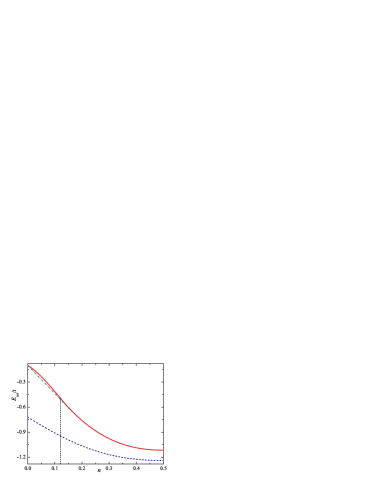
Figure 1: (Color online) Two types of behavior of the energy of homogeneous state  (8) in 2D as function of doping $n$: with a region of negative curvature (red solid line, $J/t=0.05$), and without it (blue dashed line, $J/t=0.35$); $t^{\prime}=0.5t$ for both curves. For the values of parameters corresponding to the solid curve, the orbitally canted state existing on the left-hand side of vertical line is unstable toward a phase separation. The Maxwell construction in a region of phase separation is shown by green dot-dashed line. The homogeneous state corresponding to the blue dashed curve is stable in the whole range of doping.

III Anisotropic model

Now we study a more realistic model of $e_{g}$ orbitals on the square 2D lattice. This situation is characteristic, for example, for layered cuprates, like K₂CuF₄, or manganites (La₂MnO₄ or La₂Mn₂O₇). We assume that an orbital exchange Hamiltonian has Heisenberg-like form (2). In the case of $e_{g}$ orbitals, any orbital can be written as a linear combination of two basis functions $|a>=|x^{2}-y^{2}>$ and $|b>=|2z^{2}-x^{2}-y^{2}>$: $|\theta>=\cos(\theta/2)|x^{2}-y^{2}>+\sin(\theta/2)|2z^{2}-x^{2}-y^{2}>$. The hopping integrals $t^{\alpha\beta}$ in Eq. (3) now depend on the direction of hopping, and can be written in the form of a matrix

$$(t_{x,y})^{\alpha\beta}=\frac{t_{0}}{4}\left(\begin{array}[]{cc}3&\mp\sqrt{3}\\ \mp\sqrt{3}&1\\ \end{array}\right)\,,$$ (19)

where minus (plus) sign corresponds to $x$ ($y$) direction of hopping.

Assuming again an underlying orbital structure corresponding to the alternation of $|\theta_{1}\rangle$ and $|\theta_{2}\rangle$ orbitals, we obtain the spectrum of charge carriers in the form

$$E(\mathbf{k})=-t_{0}\left(A_{x}(\theta_{1},\theta_{2})\cos k_{x}+A_{y}(\theta_{1},\theta_{2})\cos k_{y}\right)\,,$$ (20)

where

$$A_{x,y}(\theta_{1},\theta_{2})=\left|\cos\left(\frac{\theta_{1}-\theta_{2}}{2}\right)+\cos\left(\frac{\theta_{1}+\theta_{2}}{2}\pm\frac{\pi}{3}\right)\right|.$$ (21)

The total energy then reads

$$E_{tot}(\theta_{1},\theta_{2}) = t_{0}\left(A_{x}(\theta_{1},\theta_{2})+A_{y}(\theta_{1},\theta_{2})\right)\times$$ (22)

$$\varepsilon(n;\theta_{1},\theta_{2})+2J\cos(\theta_{1}-\theta_{2})\,,$$

where $\varepsilon(n;\theta_{1},\theta_{2})=\int_{-1}^{\mu}dE\,E\rho(n;\theta_{1},\theta_{2})$, and the density of states can be written as

$$\rho(n;\theta_{1},\theta_{2}) = \!\int\limits_{0}^{\infty}\!\frac{ds}{\pi}\cos(Es)\times$$

$$J_{0}\!\left(\frac{sA_{x}}{A_{x}+A_{y}}\right)J_{0}\!\left(\frac{sA_{y}}{A_{x}+A_{y}}\right)\!.$$

Note that the density of states now depends on angles $\theta_{1}$, $\theta_{2}$ via functions $A_{x,y}(\theta_{1},\theta_{2})$. In order to find orbital structure, one should minimize $E_{tot}$, Eq. (22), with respect to $\theta_{1}$ and $\theta_{2}$. The analysis shows, that at doping $n$ less than some critical value $n_{1}$, depending on the ratio $J/t_{0}$, the minimum of the total energy corresponds to $\theta_{1}=0$, $\theta_{2}=\pi$, that is, we have the homogeneous antiferro-orbital structure with alternating $|x^{2}-y^{2}>$ and $|2z^{2}-x^{2}-y^{2}>$ orbitals (we ignore here anharmonic effects and higher-order interactions, which usually stabilize locally elongated octahedra with the angles, in our notation, $\theta=\pi$, $\pm 2\pi/3$, see Refs. kanamori, ; DK, ). The energy of such a state is

$$E_{tot}=t_{0}\sqrt{3}\varepsilon_{0}(n)-2J\,.$$ (24)

This state is locally stable, $\partial^{2}E_{tot}/\partial n^{2}>0$.

At $n=n_{1}$, a jump-like transition to the canted state with $\theta_{2}=-\theta_{1}$ occurs, where

$$\theta_{1}=\arccos\left(\frac{t_{0}|\varepsilon_{0}(n)|}{4J}\right)\,,$$ (25)

and $E_{tot}(n)$ has a kink at $n=n_{1}$. The energy of such canted state at $n>n_{1}$ is

$$E_{tot}=t_{0}\varepsilon_{0}(n)-\frac{t_{0}^{2}}{4J}\varepsilon_{0}^{2}(n)-2J\,.$$ (26)

With the further growth of $n$, the angle $\theta_{1}$ decreases, and at $n=n_{2}$, determined by the equation $t_{0}|\varepsilon_{0}(n_{2})|/4J=1$, it vanishes, $\theta_{1}=0$ (ferro-OO with $|x^{2}-y^{2}\rangle$ orbitals). The total energy of the system as function of doping is shown in Fig. 2. Note, that depending on the values of parameters, the energy (26) can have either positive or negative curvature (see the inset to Fig. 2). In the former case, the homogeneous state is locally stable in the whole range of doping, but the phase separation still exists in the range of $n$ near $n=n_{1}$, due to the kink in the system energy. In the second case, PS, of course, also exists (we have an instability in some range of doping, where $\partial^{2}E_{tot}/\partial n^{2}<0$). Note, that these two possible situations (negative curvature of $E_{tot}$ and the kink) can lead to inhomogeneous states with quite different properties DiCastro .

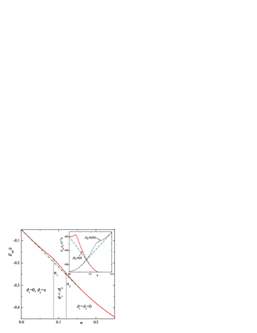
Figure 2: (Color online) The energy of homogeneous state for the anisotropic model as a functions of doping at $J/t_{0}=0.025$ (red solid curve). In the region near $n_{1}\approx 0.08$, the homogeneous state is unstable toward a phase separation. In the inset, the dependence of $E_{tot}(n)+t_{0}\sqrt{3}n$ (linear term of the dependence $E_{tot}(n)$ in the range $n<n_{1}$ is subtracted) on doping $n$ is shown at the range near $n_{1}$ at different model parameters. The red solid curve (blue dashed curve) corresponds to $J/t_{0}=0.01$ ($J/t_{0}=0.035$), and have a negative (positive) value of $\partial^{2}E_{tot}/\partial n^{2}$ in the region $n>n_{1}$ close to $n_{1}$. The phase separation exists for both situations. Maxwell construction is shown by dot-dashed line.

IV Inhomogeneities in the orbitally ordered structures

We demonstrated above that the additional charge carriers introduced to the orbitally ordered structures can lead to the formation of an inhomogeneous state. Now, let us discuss possible types of such inhomogeneities in more detail using a model of the $e_{g}$ orbitals at the sites of 2D square lattice, considered in the previous Section. We assume that each charge carrier forms a finite region of an OO structure with alternating $|\theta_{1}\rangle$ and $|\theta_{2}\rangle$ orbitals (not necessarily ferro-OO with $\theta_{1}=\theta_{2}=0$) to optimize $H_{\text{el}}$. The remaining part of the crystal has antiferro-OO structure with $|x^{2}-y^{2}>$ and $|2z^{2}-x^{2}-y^{2}>$ orbitals, according to the results of the previous Section at $n\to 0$.

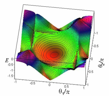
(a) $J/t_{0}=0.005$

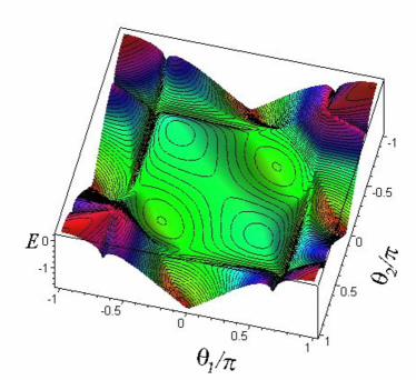
(b) $J/t_{0}=0.02$

Figure 3: Total energy as function of angles $\theta_{1}$ and $\theta_{2}$ at $J/t_{0}$ smaller (a) and larger (b) than the critical value $\simeq 0.0075$.

The spectrum of charge carriers is given by Eq. (20). Expanding this spectrum in power series of $\mathbf{k}$ up to the second order, we find an effective Hamiltonian for a charge carrier in a finite region:

$$\hat{H}_{eff}=-t_{0}\left(A_{x}+A_{y}\right)+\frac{t_{0}}{2}\left(A_{x}\frac{\partial^{2}}{\partial x^{2}}+A_{y}\frac{\partial^{2}}{\partial y^{2}}\right),$$ (27)

where $A_{x}$, $A_{y}$ are given by Eq. (21). Using Hamiltonian (27), we can solve the Schrödinger equation within a finite region, which we choose in the shape of ellipse with semiaxes $\sqrt{A_{x}}\rho_{0}$ and $\sqrt{A_{y}}\rho_{0}$. As a result, we find the following expression for the kinetic energy of the charge carrier within such droplet

$$E_{kin}=-t_{0}\left(A_{x}+A_{y}\right)+\frac{t_{0}j_{0,1}^{2}}{2\rho_{0}^{2}}\,,$$ (28)

where $j_{0,1}\cong 2.405$ is the first root of Bessel function $J_{0}$. The potential energy $E_{pot}$ related to the orbital ordering is the sum of two contributions proportional to the droplet volume $v$ ($v=\pi\sqrt{A_{x}A_{y}}\rho_{0}^{2}$): the energy of the canted OO within the droplet is $zJ\cos(\theta_{1}-\theta_{2})/2$ and the loss in energy of the antiferro-OO matrix due to the formation of the droplet is $zJ/2$. As a result, we get ($z=4$)

$$E_{pot}=4\pi\rho_{0}^{2}J\sqrt{A_{x}A_{y}}\cos^{2}\left(\frac{\theta_{1}-\theta_{2}}{2}\right)\,.$$ (29)

Minimizing the droplet energy $E_{kin}+E_{pot}$ with respect to $\rho_{0}$, we find

$$\rho_{0}=\left(\frac{t_{0}j_{0,1}^{2}}{8\pi J\sqrt{A_{x}A_{y}}\cos^{2}\left(\frac{\theta_{1}-\theta_{2}}{2}\right)}\right)^{1/4}\!\!.$$ (30)

The total energy (per lattice site) then reads

$$E_{tot} = -2J+E(\theta_{1},\,\theta_{2})\,n\,,$$ (31)

$$E(\theta_{1},\,\theta_{2}) = -2t_{0}(A_{x}+A_{y})\phantom{\frac{1}{2}}$$

$$+j_{0,1}\left(8\pi t_{0}J\sqrt{A_{x}A_{y}}\right)^{1/2}\left|\cos\left(\frac{\theta_{1}-\theta_{2}}{2}\right)\right|,$$

where we assume that all charge carriers introduced by doping form such identical OO droplets.

To find possible types of OO droplets, we minimize $E$ with respect to $\theta_{1}$ and $\theta_{2}$ (note again, that functions $A_{x,y}$ depend on $\theta_{1}$, $\theta_{2}$ according to Eq. (21)). The function $E(\theta_{1},\,\theta_{2})$ at two different values of $J/t_{0}$ is shown in Fig 3. In general case, the function $E(\theta_{1},\,\theta_{2})$ has several minima, and the values of $\theta_{1}$ and $\theta_{2}$ corresponding to the lowest minimum depend drastically on parameter $J/t_{0}$. At small $J/t_{0}$ (Fig 3a), the lowest minimum corresponds to $\theta_{1}=\theta_{2}=0$, that is, we have ferro-OO structure inside the droplet with occupied $|x^{2}-y^{2}>$ orbitals. In this case, the most favorable shape of droplets is a circle (see left panel of Fig. 4). At $J/t_{0}$ larger than some critical value ($J_{cr}/t_{0}\simeq 0.0075$), the minimum $\theta_{1}=\theta_{2}=0$ becomes metastable, and the energy $E(\theta_{1},\,\theta_{2})$ has four degenerate lowest minima: two of them correspond to $\theta_{1}=\pi/3$, $\theta_{2}=2\pi/3$, $\theta_{1}=-\pi/3$, $\theta_{2}=-2\pi/3$, and the similar two minima with the replacement $\theta_{1}\leftrightarrow\theta_{2}$ (see Fig 3b). In this case, we have chains of alternating $|x^{2}-z^{2}>$ and $|2y^{2}-x^{2}-z^{2}>$ (or $|y^{2}-z^{2}>$ and $|2x^{2}-y^{2}-z^{2}>$) orbitals and hence nearly one-dimensional (cigar-shaped) droplets stretched along $y$ or $x$ axes (right panel of Fig. 4). With the further growth of $J/t_{0}$ the metastable state $\theta_{1}=\theta_{2}=0$ splits into two states corresponding to $\theta^{*}_{1}=-\theta^{*}_{2}$ with positive and negative $\theta^{*}_{1}$, as it can be seen from Fig 3b. The droplets corresponding to these states have circular shape, but canted OO structure.

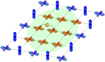
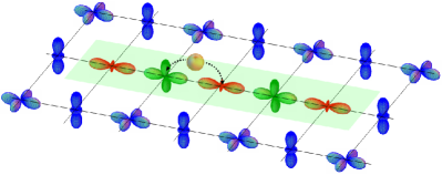
Figure 4: (Color online) Schematic illustration of circular (left panel) and needle-like (right panel) droplets. An electron or hole moves in a finite region creating a ferro- or canted-OO structure, in antiferro-OO matrix. In the case of hole, there exists a one mobile empty site within a droplet.

The existence of two types of droplets with different shapes can be easily understood. The maximum gain in the kinetic energy corresponds to the ferro-OO state with $|x^{2}-y^{2}>$ orbitals. At small $J/t_{0}$, the kinetic energy prevails, and we have circular droplets with this type of orbitals. The minimum cost in the potential energy corresponds to nearly one-dimensional structures. At larger $J/t_{0}$, the potential energy plays more important role than the kinetic one, and we get cigar-like droplets (smaller volume of such a droplet gives smaller loss of orbital energy). The orbital structure inside the droplet described above corresponds to the maximum gain in the kinetic energy for one-dimensional chain (in the absence of hopping between neighboring chains).

The analysis shows, that the energy of an inhomogeneous state, Eq. (31), consisting of circular or cigar-like OO droplets embedded into an antiferro-OO matrix is less than the energy of a homogeneous state in a certain range of doping $0<n<n^{*}_{c}$. With the growth of the number of charge carriers, the droplets start to overlap, and at $n=n^{*}_{c}$ the inhomogeneous state of considered type (ferro-OO droplets in antiferro-OO matrix) disappears. However, the phase separation exists in a wider range of doping (see the previous Section). For circular droplets, we have an estimate $n^{*}_{c}\sim 1/\pi\rho_{0}^{2}$. Taking for estimate the ratio $J/t_{0}=0.005$, we get $\rho_{0}\approx 2$ (in units of lattice constant) and $n^{*}_{c}\sim 0.08$.

In the case of cigar-like droplets, we have $A_{x}=0$ (or $A_{y}=0$), and according to Eq. (30) we would get that chains have infinite length (but zero volume $v$), $\rho_{0}=\infty$. This is of course not a very realistic result, coming from an approximation, where the potential is assumed to be proportional to the droplet volume only. In order to estimate the characteristic length $L$ of the chain, we should take into account the surface term (proportional to the droplet’s length) in the potential energy $E_{pot}$ of the droplet. Let us consider, for definiteness, the chain of $|y^{2}-z^{2}>$ and $|2x^{2}-y^{2}-z^{2}>$ orbitals, stretched along $x$ axis. In this case, we have $A_{x}=\sqrt{3}$, $A_{y}=0$. The effective Hamiltonian (27) is reduced to

$$\hat{H}_{eff}=-t_{0}\sqrt{3}+\frac{t_{0}\sqrt{3}}{2}\frac{\partial^{2}}{\partial x^{2}}\,,$$

and the kinetic energy of the charge carrier in the chain of length $L$ becomes $E_{kin}=-t_{0}\sqrt{3}(1-\pi^{2}/2L^{2})$. The surface energy of interorbital exchange interaction has a minimum, when the chain is located in an antiferro-OO matrix like shown in Fig. 4: each $|y^{2}-z^{2}>$ ($|2x^{2}-y^{2}-z^{2}>$) orbital in the chain has its nearest neighbor $|x^{2}-y^{2}>$ ($|2z^{2}-x^{2}-y^{2}>$) orbital in the matrix. In continuum approximation, the potential energy can be written as $E_{pot}=9JL/4$. Minimizing $E_{kin}+E_{pot}$ with respect to $L$, we arrive at the following formula for characteristic length of the chain:

$$L_{0}=\left(\frac{4\pi^{2}t_{0}\sqrt{3}}{9J}\right)^{1/3}\!\!.$$ (33)

At $J/t_{0}=0.05>J_{cr}/t_{0}$, we have $L_{0}\approx 5.5$. At random distribution of the chains in the matrix (we have chains stretched both along $x$ and $y$ axes), the critical concentration is about $n^{*}_{c}\sim 1/L_{0}^{2}$, but it can be larger if a more complicated structure of chains, e.g. regular stripes, appears in the system.

V Conclusions

We have studied a simple model of electronic phase separation in the system of charge carriers moving in an orbitally ordered background. It was shown that a homogeneous state in such a system can be unstable toward a phase separation, where delocalized charge carriers favor the formation of nanoscale inhomogeneities with the orbital structure different from that in the undoped material. The shapes and sizes of such inhomogeneities were determined for 2D lattice of $e_{g}$ orbitals. The shape of inhomogeneities depends drastically on the ratio of interorbital exchange interaction and a hopping amplitude of the charge carriers, $J/t_{0}$: there exists a critical value of $J/t_{0}$, corresponding to the transition from the circular inhomogeneities to a one-dimensional chains of finite length.

The model under study is quite similar to the double exchange model, where the orbital variables play a role of local spins. It is well known that such a model also exhibits an instability toward a phase separation into phases with different types of magnetic ordering. The inhomogeneous state with circular ferro-OO droplets is, in essence, an analog of a magnetic polaron state (ferromagnetic droplets in an antiferromagnetic matrix), which is usually considered in the double exchange model Nag ; Kak ; KaKhoMo . Nevertheless, our orbital model is more complicated than the usual double exchange due to the existence of non-diagonal hopping amplitudes and to the anisotropy in hoppings. Both these features lead to the results specific for the orbital model, such as the kink in the energy of a homogeneous state and canted-OO needle-like droplets.

In the present paper, any magnetic structure and spins of the charge carriers were fully neglected. Taking into account spin degrees of freedom can lead to the formation of inhomogeneities with different orbital and spin configurations.

In the proposed model, the localized electrons forming an orbital order and the conduction electrons or holes were supposed to be two different groups of electrons. However, we can argue that our main results are also valid for a model, where the same electrons take part both in the hopping and in the formation of orbital ordered structure. Indeed, in the case of magnetic oxides with Jahn-Teller ions, an orbital degeneracy is lifted by lattice distortions, giving rise to an orbitally-ordered ground state at $n=1$. If we suppose that a long-range orbital ordering still exists at small hole doping $x=1-n\ll 1$, we come to the situation considered in present paper: we have holes moving in an orbitally-ordered background. In a mean-field approximation, we only should replace in all formulas above $n\to x=1-n$ and $J\to J(1-x)^{2}$, since the number of sites taking part in interorbital exchange interaction is reduced by a factor of $1-x$ . In the materials with Jahn-Teller ions, the orbital Hamiltonians are more complicated than the Heisenberg-like Hamiltonian considered in this paper. Preliminary calculations for the Hamiltonian corresponding to the superexchange mechanism of the orbital ordering KK show that the obtained results remain qualitatively the same. However, in real substances, there also exists a possibility of OO without local distortions, corresponding to complex combinations of $e_{g}$ orbitals vBrK2001 , which needs a special analysis.

References

- (1) Also at the Department of Physics, Loughborough University, Leicestershire, LE11 3TU, UK.
- (2) K.I. Kugel and D.I. Khomskii, Usp. Fiz. Nauk 136, 621 (1982) [Sov. Phys. Uspekhi 25, 231 (1982)]
- (3) M.D. Kaplan and B.G. Vekhter, Cooperative Phenomena in Jahn-Teller Crystals (Plenum, New York, 1995).
- (4) E. Dagotto, Nanoscale Phase Separation and Colossal Magnetoresistance: The Physics of Manganites and Related Compounds (Springer-Verlag, Berlin, 2003).
- (5) E. Nagaev, Colossal Magnetoresistance and Phase Separation in Magnetic Semiconductors (Imperial College Press, London, 2002).
- (6) M.Yu. Kagan and K.I. Kugel, Usp. Fiz. Nauk. 171, 577 (2001) [Physics - Uspekhi 44, 553 (2001)].
- (7) R. Kilian and G. Khaliullin, Phys. Rev. B60, 13458 (1999).
- (8) T. Mizokawa, D.I. Khomskii, and G.A. Sawatzky, Phys. Rev. B63, 024403 (2000).
- (9) G. Khaliullin and S. Okamoto, Phys. Rev. Lett. 89, 167201 (2002).
- (10) J. van den Brink, G. Khaliullin, and D. Khomskii, Orbital effects in manganites, Ch. 6 in Colossal Magnetoresistive Manganites, ed. T. Chatterji, (Kluwer, Dordrecht, The Netherlands, 2004), pp. 263-302.
- (11) M.Yu. Kagan, D.I. Khomskii, and M.V. Mostovoy, Eur. Phys. J. B 12, 217 (1999).
- (12) J. Kanamori, J. Appl. Phys. 31, 14S (1960).
- (13) D. Khomskii and J. van den Brink, Phys. Rev. Lett. 85, 3329 (2000).
- (14) C. Ortix, J. Lorenzana, and C. Di Castro, arXiv:0801.0955 (2008).
- (15) J. van den Brink and D. Khomskii, Phys. Rev. B63, 140416(R) (2001).